Abstract
Important to the success of additive manufacturing (AM) is the ability to inspect and qualify parts. The research community is pushing to identify correlations between part function and surface topography, yet little guidance specific to AM surface measurement exists. Thus, development of inspection methods for surface finish are required. In laser powder bed fusion (LPBF) AM, parts are built through a complex process with many variables, and the length scales of interest on the surface cover a wide range. Full characterization of the surface is time consuming and costly as high resolution in surface measurements decreases field-of-view (FoV), requiring stitching multiple FoVs to cover large areas. Statistical methods exist to estimate the maximum value based on a sample of FoVs, but are not yet commonplace in AM surface measurement. The goal of this work is to understand the use of these statistical methods in the estimation of maximum area valley depth () of a surface, an extreme value parameter, for which researchers have already found relationship to fatigue life. This work also investigates the effect of microscope objective, measurement region size, and nesting index of areal filters on . A large (i.e., greater than 40 mm × 40 mm) planar LPBF surface is fabricated in nickel superalloy 625 and measured using a focus variation microscope with a objective and again with a objective. Results show that there is little difference in the maximum value of between the two objectives, but the nesting index does have some effect. Results also show that a Type 1 Generalized Extreme Value, or Gumbel, distribution can be used to accurately estimate the maximum value of for a surface from a small set of measurements, providing a framework for users to develop inspection routines that balance measurement time and accuracy of estimation.
Keywords: Additive manufacturing, extreme value, laser powder bed fusion, maximum area valley depth, surface metrology
Introduction
Due to the ability to reduce time-to-market and cost to manufacture, a key technology for production of complex and high-value parts has been additive manufacturing (AM) [1,2]. With the ability to produce fine detail in finished parts compared to other AM technologies, laser powder bed fusion (LPBF) has generated a great deal of interest [3]. However, a limitation hindering the widespread adoption of AM is the as-built surface topography and the difficulty in determining its effect on part performance. While performance indicators exist for other metal manufacturing processes, it is not yet clear how these indicators can be translated to AM processes. As such, the development of functional correlations to surface topography and stronger understanding of corresponding measurement techniques has been cited as a knowledge gap by multiple standardization roadmaps [4,5]. The research community has responded to this limitation through investigations of AM surface topography to characterize relationships to the process physics and to correlate the surface to function and numerous studies are presented in the review articles by Townsend et al. [6] and Leach et al. [7].
Relevant to this publication, Kleszczynski et al. determined the importance of laser incident angle on the profile average roughness (Ra) of downward facing parts [8]. This was later confirmed by Rott et al. with more detailed analysis of the laser incident angle [9]. Fox et al. found that the parameter Ra provides little benefit to more nuanced characterization of downward facing surfaces beyond changes in build angle, but other available parameters, such as the mean width of profile elements (Rsm) and profile peak density (Rpc) may be useful [10,11]. Triantaphyllou et al. [12] found that parameters such as the area average roughness (), the area root mean square roughness (), and area skewness () could be used to identify the difference between upskin and downskin surfaces, but additional research is required to confirm the usefulness of these parameters. Work by Fox et al. [10] found that there is little statistical difference in the Ra parameter for surfaces with drastically different topographies so it follows that the usefulness of the areal parameter may be limited as well.
The research community is also actively investigating relationships between part function and surface topography. Stimpson et al. investigated the effect of as-built surface finish on the heat transfer in AM channels [13]. Gockel et al. found correlation between the maximum area valley depth () and the number of cycles to failure in axial fatigue tests, while showed no correlation [14]. Similarly, Zhang and Fatemi investigated the effect of surface roughness on multiaxial fatigue of Ti-6Al-4V samples, finding correlation to the maximum profile valley depth (Rv) [15].
Through the investigations into process-structure-property (PSP) relationships for AM, it has become clear that the existing measurement methods (i.e., those laid out in ASME B46.1 [16], ISO 4287 [17], and ISO 25178 [18]), require additional scrutiny to be effective. For example, as previously mentioned, Fox et al. [10] found that there is little statistical difference in the Ra parameter for surfaces with drastically different topographies. Triantaphyllou et al. [12] found that the 2.5 mm L-filter nesting index was sufficient to capture the required data for use of parameters , , and , suggesting that the 8.0 mm L-filter nesting index may not be required. Other studies have successfully investigated the use of more complex methods, such as feature based characterization [19] and segmentation [20]. These methods, and others, also benefit from the development of relationships between the process and resultant features (e.g., those depicted in Strano et al. [21], Cabanettes et al. [22], and Tian et al. [23]) as they provide a general expectation that can inform more focused analysis.
Issues in developing PSP relationships are also complicated by the plethora of technologies used for the measurement of surface finish, whose bandwidth characteristics vary [24]. Thompson et al. [25] investigated the agreement and discrepancy between various technologies in the measurement of top surfaces of an AM part. They found that that these comparisons, while currently too limited to provide guidance on the most appropriate technology for measurement of AM surfaces, will be vital to improving our understanding of topography measurement artifacts and their effect on texture parameters. Zanini et al. [26,27] compared optical and X-ray computed tomography (XCT) surface measurements against twodimensional (2D) cross-sectional profiles, noting that the re-entrant features of AM surfaces significantly affect the accuracy of optical measurements. Fox et al. [28,29] investigated the registration of optical surface measurements and three-dimensional (3D) XCT measurements for more information-rich metrology (a term coined by Leach et al. [30]). While findings were too limited to provide insight into a relationship between surface texture and subsurface porosity, a key finding was that users should be cautious of sub-voxel rescaling of XCT measurements as it provided little to no improvement over the original voxel size data in comparison to laser confocal measurements. This observation is also confirmed in Thompson et al. [25], who investigated the effect of magnification and sampling resolution in XCT of metal AM surfaces, finding that geometric magnification has a stronger effect than sampling resolution.
Still, there is inadequate knowledge in the AM research community of appropriate methods for characterization of AM surfaces [31]. Standards from ASME [16] and ISO [17,18], as well as an extensive library of Good Practice Guides from the National Physical Laboratory [32], guide the evaluation of traditionally manufactured surface topography but it is still unclear how well these methods will apply to as-built AM surfaces. Gomez et al. presented insights and recommendation for optimization of metal AM surface measurements using coherence scanning interferometry (CSI) through use of advanced measurement functions (e.g., signal oversampling, high dynamic range lighting levels, sophisticated topography reconstruction algorithms, etc.) that are available from equipment manufacturers [33]. Newton et al. [34] explored the effect of measurement control parameters (e.g., objective, illumination, vertical and lateral resolution settings) on the measurement of AM surfaces using focus variation microscopy and found that these settings had little effect on the areal parameter but did see changes in local repeatability and the percentage of non-measured points. ASTM currently has a work item to develop guidance for measurement of AM surfaces [35] and the ASME B46 committee has a project team (PT53) dedicated to determining the changes required of the B46.1 standard to address AM surfaces; however, little guidance is currently provided on how to appropriately characterize AM surfaces. Thus, without a strong understanding of the required fidelity, point spacing, measurement size, etc., it can be difficult to determine the quality of the correlations found in research.
Additionally, length scales of interest in AM can be vast making detailed characterization of larger surfaces difficult. Statistical modeling and sampling techniques can be leveraged to characterize an entire part surface using only measurements from a small fraction of it. Sampling techniques include completely at random, stratified, and systematic. These techniques help to ensure the representativeness of the sample, increasing our confidence that an important part of the surface has not been overlooked. Moreover, these sampling techniques provide the structure on which the assumptions of probabilistic models may rest, and these models are used to make predictions about the part surface, which is the analysis goal. Manufacturing industries have been using statistical modeling and sampling techniques for quality control for many years. For that reason, prior work by the authors [31] investigated the effect of sampling strategy on the areal parameter , finding that random sampling across the surface performed better than contiguous sampling for representing a large surface with a small sample of measurements. That work also found additional evidence that measurement size should be dictated by the maximum spatial wavelength of interest.
With these aspects in mind, the purpose of this research is to investigate the effect that measurement and sampling strategies have on calculated areal surface parameters, as well as the ability to adequately represent a large surface measurement from a set of sampled regions. We focus on extreme value parameters in surface analysis. A part made from nickel superalloy 625 (IN625) with a large (over 40 mm × 40 mm) planar surface was measured in a focus variation (FV) system with multiple focusing objectives. The data from these surface measurements are subdivided into common measurement region sizes based on various numbers of stitched field-of-views (FoVs). Random samples of subdivided measurement regions in varying quantities are analyzed to determine the ability of the sample(s) to represent the entire surface. This work provides a framework for developing measurement routines in the qualification of AM parts.
Methods
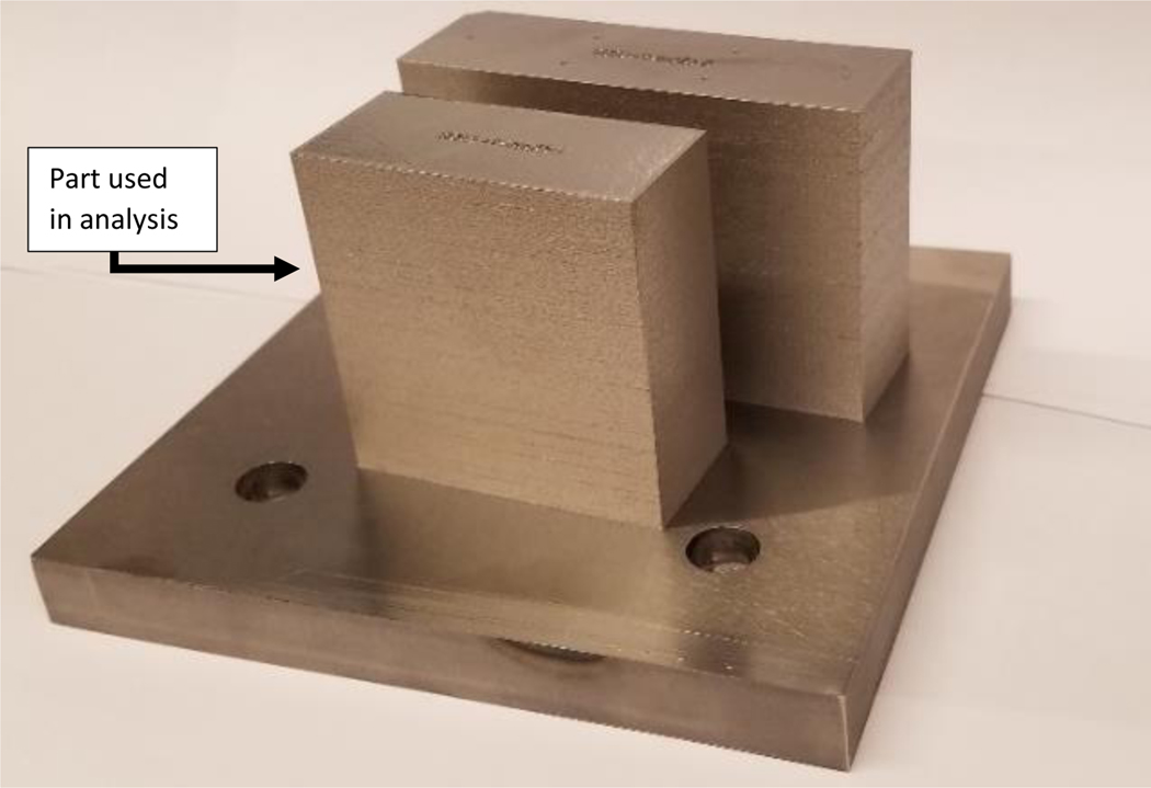
The part and data used for this research is the same used in prior work by the authors [31]. The part, which is shown in Figure 1, was fabricated on an EOS M290 system at the National Institute of Standards and Technology (NIST) using the vendor recommended parameter settings. The part was designed as a 55 mm × 55 mm × 25 mm block. The feedstock material used for the study was the commercially available EOS NickelAlloy IN625, which corresponds to the unified numbering system (UNS) classification N06625 [36]. For the remainder of this manuscript, the material will be abbreviated as IN625. Material used for the build was powder reclaimed from prior builds using an 80 μm sieve.
Figure 1.
Part used for the analysis (in the foreground). The larger block in the background was not used in this analysis. Dimensions of the substrate are 12.7 cm × 12.7 cm × 1.3 cm [31].
All areal surface height measurements used in this study were taken from the large vertical surface of the part (i.e., the 55 mm × 55 mm surface) whose orientation is nominally perpendicular to the top of the build substrate. Height measurements were taken using an Alicona InfiniteFocus G5 focus variation (FV) microscope, which conforms to ISO 25178–606:2015 [37]. Coaxial and ring (i.e., off-axis) lighting was used and settings (e.g., intensity, brightness and contrast) were optimized for each measurement. A objective with numerical aperture (NA) of 0.3 and objective with NA of 0.4 were used in the analysis. Point spacings for the and objectives were approximately 0.88 μm and 0.44 μm, respectively, which are smaller than the optical lateral resolution limit for each objective (i.e., 1.09 μm for the objective and 0.82 μm for the objective [38]). The microscope’s sensor captures data as an 1840 pixel × 1840 pixel grid for a single field-of-view (FoV). Thus, a single FoV measures 1.62 mm × 1.62 mm for the objective and 0.81 mm × 0.81 mm for the objective.
To create the large measurement dataset for this study, and were stitched for the and objectives, respectively, creating measurement regions greater than 40 mm × 40 mm while maintaining the previously mentioned point spacings. The additional FoV for the objective measurements (e.g., instead of ) was captured to reduce errors in alignment of measurements with the objective and objective; however, that analysis was not performed in this work. Measurements were taken at a minimum of 5 mm away from any edge of the part to minimize the effect of the part geometry on the surface texture. Three separate measurements were taken one after another for each objective to be averaged later to reduce the effect of measurement noise. For example, a measurement with the objective was taken, stitched, and saved by the equipment and this process was repeated two more times before replicating the process with the objective.
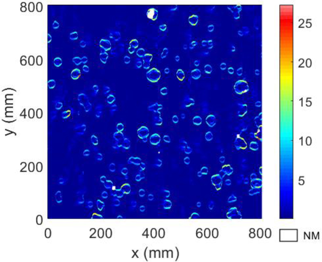
Measurements were exported from the microscope’s software as 16-bit gray scale images, the highest resolution option for saving and exporting a measurement region of this size. In this export method, heights are mapped to 16-bit integers where the minimum height corresponds to zero, and the maximum height 216 − 1. This discretization led to a rounding of the vertical spacing to approximately 3.7 nm and 3.4 nm for the and objectives, respectively. The influence on the result should be negligible as this is an order of magnitude lower than the stated height resolution of the equipment (50 nm for the objective) [38]. Once the three measurements with the objective and three 60 FoV × 60 FoV measurements with the objective were exported as an image, the three height values for a given objective at each (x,y) location were averaged to reduce noise. Analysis of the three data points at each (x,y) location over the entire measurement area was performed and an average standard deviation of 0.96 μm and 1.09 μm for the and objectives, respectively, was found. A subset of this analysis taken from the upper left corner of the measurement area with the objective is shown in Figure 2. In this analysis, large standard deviations near the borders of powder particles (e.g., where steep drops occur) were found where values eclipse 25 μm. This variation is likely due to errors in the (x,y) positioning between the three measurements.
Figure 2.
Example of the standard deviation calculated for each (x,y) location from the three measurements performed with the objective. “NM” represents the non-measured points.
The averaged data was then subdivided into smaller measurement samples using MATLAB. The height data was subdivided into the smaller measurement regions based on equivalent stitched FoVs and assuming a 10 % overlap for the stitching. The associated measurement region sizes are presented in Table 1.
Table 1.
Lateral size of measurement samples after stitching.
| Lateral Size of Measurement Sample | |||
|---|---|---|---|
| Stitched FoVs | Pixels | obj. (mm) | obj. (mm) |
| 1840 | 1.62 | 0.81 | |
| 3496 | 3.08 | 1.53 | |
| 5152 | 4.54 | 2.26 | |
| 6808 | 5.99 | 2.98 | |
| 8464 | 7.45 | 3.71 | |
| 10120 | 8.91 | 4.44 | |
| 13432 | 11.82 | 5.89 | |
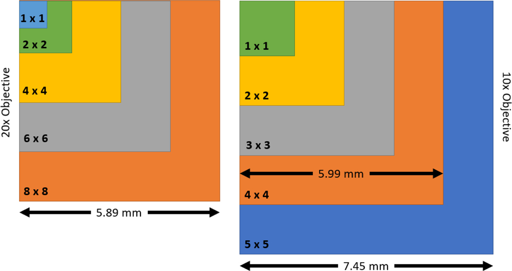
While the magnifications are such that at FoV with the objective is twice the size of a FoV with the objective, the overlap distance required for stitching creates a difference in the overall size. This difference is illustrated in Figure 3.
Figure 3.
Illustration of the difference in approximate measurement sizes of stitched FoVs for the objective (left) and objective (right) assuming a 10% overlap.
When subdividing the full measurement of the surface into smaller measurement regions, using the measurement sizes listed in Table 1, the number of measurement regions that fit into the full measurement of the surface are listed in Table 2. Due to the required overlap during stitching of the measurement region, the final measured area is reduced to a corresponding 26 FoV × 26 FoV. The measurement regions (e.g., FoV, FoV, etc.) from the subdivision do not overlap one another in the full measurement space since we are partitioning the already stitched measurement.
Table 2.
Number of measurement samples after subdividing the full area measured. Numbers marked as N/a were not used in this analysis either for brevity or due to memory limitations of the analysis computer.
| Objective | Objective | |||
|---|---|---|---|---|
| Stitched FoVs | Count in x, y | Total | Count in x, y | Total |
| 26 | 676 | 52 | 2704 | |
| 13 | 169 | 27 | 729 | |
| 9 | 81 | N/a | N/a | |
| 7 | 49 | 17 | 289 | |
| 5 | 25 | N/a | N/a | |
| N/a | N/a | 9 | 81 | |
| N/a | N/a | 7 | 49 | |
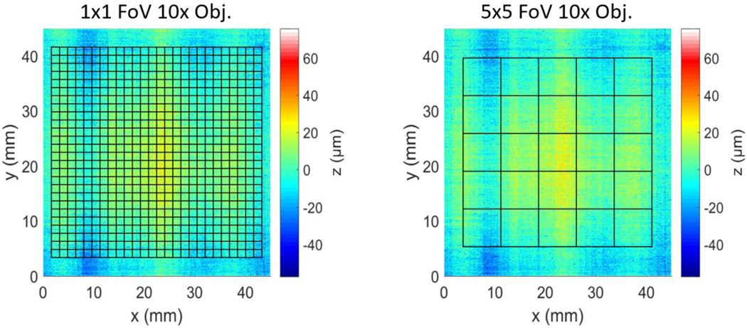
To determine positions of the subdivided samples, the set of measurement samples in a square array were centered in the full area of available data and any excess data that could not form a full FoV around the perimeter was neglected from the analysis. For example, for the objective with a FoV size, 13.68 samples × 13.68 samples can fit in the full measurement area. Thus, an array of 13 samples × 13 samples centered in the full measurement area was extracted and the excess data around the perimeter was neglected. An example of the how this layout changes for each measurement sample size is shown in Figure 4 using the FoV and FoV measurement sizes with the objective.
Figure 4.
Comparison of the layout of FoV and FoV measurement sizes using the objective, overlaid on the full measurement dataset.
Once the data were subdivided they were exported from MATLAB, converted to the X3P format [39], and imported into the commercially available OmniSurf3D software [40]. The data were leveled by a least squares plane reference geometry using vertical residuals and outliers were removed using a standard deviation cutoff of 5.0. This setting for the outlier removal was chosen as smaller values noticeably began to remove features of the topography that were not attributed to noise (i.e., the tops of apparent powder particles). Prior to the calculation of parameters, the data were filtered using digital Gaussian filters. An analysis of filters is performed, and the filter settings are described in the Comparison of Objectives, Filters, and Measurement Region Sizes section. For the remainder of the analysis, which focuses on the objective data, nesting indices of S-filter = 2.2 μm and L-filter = 0.405 mm are used. The 2.2 μm S-filter was chosen because it is five times larger than the point spacing (0.44 μm), per guidance in ISO 25178–3 [41] and ASME B46.1 (2019) [16]. The 0.405 mm L-filter because it is half the lateral size of the smallest FoV region size (0.81 mm for the FoV with the objective). This is smaller than the guidance provided in ISO 25178–3 [41]; however, recommendations for a filter cutoff at half the lateral size are seen in ASME B46.1 (2019) [16]. While this guidance is not specifically for areal measurements of AM surfaces, the fundamental reasoning behind these choices is still valid for comparing the various FoV region sizes and half the lateral size was chosen to be the more conservative selection. While the choice of data preparation, including but not limited to outlier removal and filter selection, is expected to affect the resulting calculated parameters, it does not affect the statistical methods presented in the next section. Nevertheless, more detailed analysis of the effect these choices for discrimination of surfaces is suggested for future work and discussion of the effect of measurement uncertainty on the results is presented in the Limitations of the Study section.
Statistical methods
The probability distribution for the maximum value of a sample of independent and identically distributed observations converges to the generalized extreme value (GEV) distribution as the sample size increases. The GEV distribution connects three separate probability distributions often referred to as Type 1, 2, and 3, or Gumbel, Frèchet, and Reversed Weibull, respectively. They were first identified for this purpose almost 100 years ago by Fisher and Tippett [42]. These three distributions differ most markedly in their tail behavior, i.e., the amount of probability that is placed far away from the central mass of the distribution. The Reversed Weibull distribution places positive mass on the interval (-infinity, u), with u finite. It is said to have a light upper tail since zero probability is placed above u. The Frèchet distribution places positive mass on the interval (l, infinity) with l finite. In some cases, while it is always a proper probability distribution, so much probability is placed on very large positive numbers that the mean is infinite. Thus, it is said to have a heavy upper tail. The Gumbel distribution places positive probability on all real values and the amount of mass it places on very large numbers is a compromise between the Reversed Weibull and Frèchet distributions.
The Gumbel distribution is important in engineering applications such as the current one. This is because in engineering applications, measurements often cannot be arbitrarily large. An upper bound exists, but it may not be known precisely. For example, in the current application, any measurement of the depth of a valley on the surface must be less that the depth of the part itself. That is an upper bound, but it is much too large. For these situations, the Reversed Weibull distribution may be the most appropriate of the three extreme value distributions. In practice, however, it is very difficult to estimate the upper bound from a finite sample, and if safety is crucial, it may be unwise to try to do so. Since the Gumbel distribution has the lightest infinite tail of the three distributions, it often used in place of the Reversed Weibull distribution.
The probability density function of the Gumbel distribution is given in Equation (1) and it has two parameters, and , corresponding to the distribution’s location and scale, respectively. The mean of the Gumbel distribution is , where and is the Euler-Mascheroni constant [43]. The standard deviation is . Using a sample of three or more maxima, the values of and , and their standard errors may be estimated using maximum likelihood (see Casella and Berger, 2002, pages 315 and 496) [44]. The likelihood function is the product of Gumbel probability density functions, with one term for each observed maximum.
| (1) |
Results and Discussion
In surface topography of AM parts, the Gumbel distribution is an appropriate model for both the maximum area peak height () and the maximum area valley depth (). The results to follow will focus on the parameter . The purpose for investigating in this paper is due to its relationship to fatigue found in other research by Gockel et al. [14]. However, it is anticipated that the relationships found here will hold for other extreme value parameters.
Comparison of Objectives, Filters, and Measurement Region Sizes
Using the measurements from both microscope objectives, a comparison of the calculation of the maximum from all the available data for varying FoV region sizes is presented in Table 3. In order to match bandwidths between the two objectives and multiple FoV region sizes, digital Gaussian filters with nesting indices of S-filter = 4.4 μm and L-filter = 405 μm were used. Since the point spacing of the objective data is 0.88 μm and the width/height of the objective FoV is 0.81 mm, all the measurements in the Table 3 will meet the criteria described in the Methods section.
Table 3.
Comparison of maximum values for and objective data subdivided into various FoVs. Similar sizes of measurement regions in terms of millimeters are listed adjacent to one another (e.g., the FoV is similar in size to the FoV).
| FoV | (μm) | FoV | |
|---|---|---|---|
| 40.8 | |||
| 41.7 | 40.5 | ||
| 41.6 | 40.6 | ||
| 41.6 | 40.4 | ||
| 42.6 | 41.1 | ||
| 41.6 | |||
From the data presented in Table 3, little difference, compared to the magnitude of the maximum value, can be seen in the data from the various measurement objectives and FoV region sizes when the same filters are applied to all of the data. This comparison, however, is without considering differences in uncertainty between the two objectives. Though these values are similar, the uncertainty is expected to change between the two objectives and should be considered in any analysis. The steep slopes typically seen in as-built AM surfaces should contribute to these differences [25]. For one, the steep slopes create difficulty in returning light that is reflected outside the NA of the objective, though advances continue to minimize this limitation [45]. While FV systems are capable of up to 80° slope in idealized examinations [46], it is not clear how well this will translate to the measurement of actual AM surfaces. Additionally, changes in resolution between the two objectives are expected to be relevant as the powder diameters are on the order of tens of micrometers and FV has been shown to have difficulty capturing the spherical shape [19]. Thus, the study of this issue is suggested for future work and the Limitations of the Study section contains additional discussion of the effect of uncertainty on the methods presented.
As a continuation, an analysis of various L-filter sizes is shown for the objective in Table 4. For this analysis, an S-filter of 2.2 μm (e.g., five times the 0.44 μm point spacing of the objective) was used. From this data, again there is little difference in the maximum value of when changing measurement region size and maintaining filter settings. There is, however, an increase in as the L-filter increases. While this increase is inconsequential to the statistical analyses presented in the subsequent sections, it motivates future work in understanding how long wavelength surface variations affect .
Table 4.
Analysis of the effect of L-Filter selection on the maximum value of from all the available data.
| (μm) | L-Filter (mm) | ||||
|---|---|---|---|---|---|
| FoV | 0.405 | 0.765 | 1.49 | 2.22 | 2.945 |
| 40.8 | N/a | N/a | N/a | N/a | |
| 40.6 | 45.1 | N/a | N/a | N/a | |
| 41.2 | 43.0 | 46.4 | N/a | N/a | |
| 40.6 | 43.6 | 46.7 | 47.4 | N/a | |
| 41.5 | 45.4 | 48.9 | 50.8 | 52.0 | |
Distribution of the Extreme Value Surface Parameter
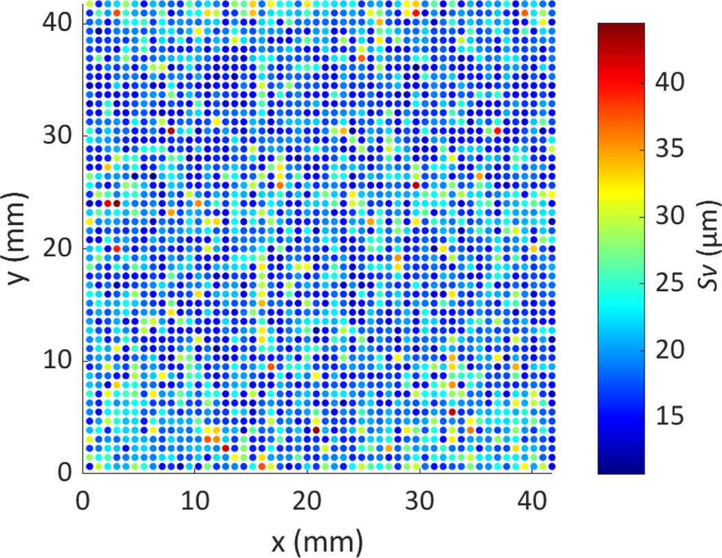
We can investigate the variation of across the surface. Figure 5 shows from the objective data, subdivided into the FoVs from the entire measured surface. Note that while various filters were analyzed in the previous section, the filters and settings described in the methods section will be used for the remaining analyses. Since there is no functional performance objective to these measurements, the selection of filters is of no consequence if they are consistent among all measurement region sizes.
Figure 5.
Calculation of areal parameter using the objective data, subdivided in to FoVs. Data is displayed by their location on the surface, which is denoted by the x and y axes.
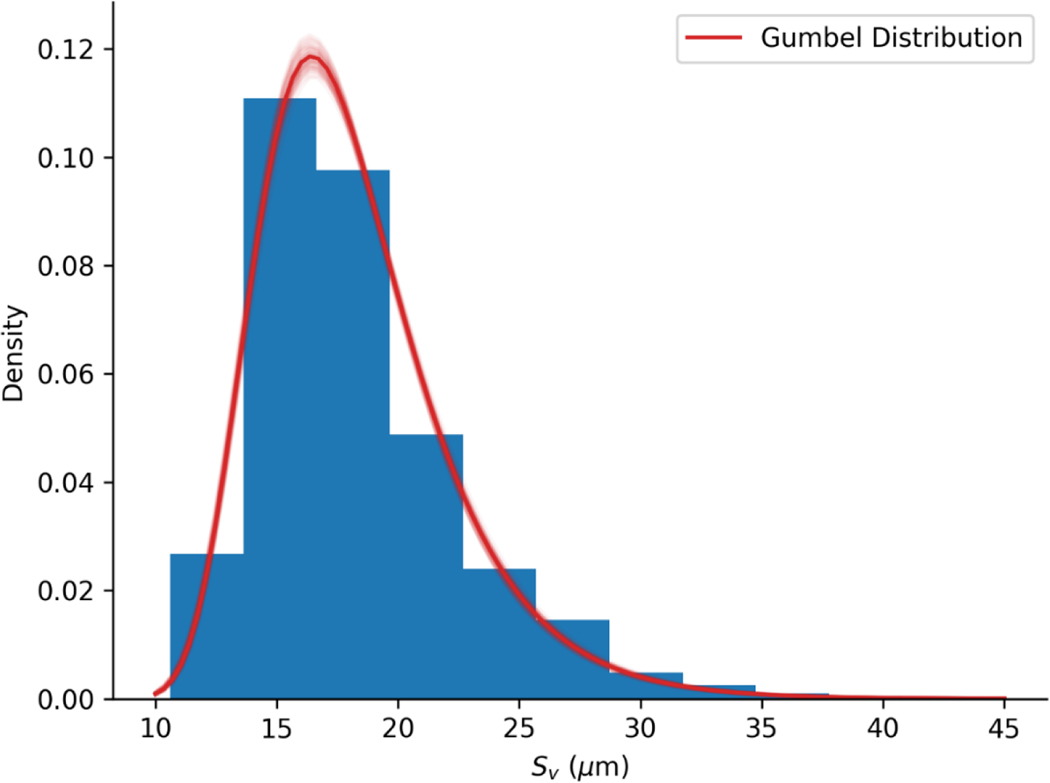
From this figure, we can see that there is a large spread in values. However, in situations where is correlated to function, the maximum value (or a small set of the largest values) is most important. The maximum value from this dataset is 40.8 μm. A histogram of all values, the Gumbel distribution fitted to them, and uncertainty associated with the fitted Gumbel distribution is shown in Figure 6. The code used for fitting the Gumbel distribution is supplied in Appendix: Python Code for Gumbel Distribution Fit.
Figure 6.
Histogram of values in the FoV dataset, the Gumbel distribution fitted to them (dark red curve, and uncertainty associated with the fitted Gumbel distribution (light red curves). Uncertainty is depicted by 50 replicate Gumbel distributions, where a replicate is obtained by perturbing the maximum likelihood estimates of and by a multivariate normal vector with mean zero, and covariance matrix given by the negative inverse of the Hessian matrix of the likelihood function evaluated at its maximum.
In extreme value analyses, estimates of maximum values, otherwise known as return values, are often of interest. In topography of AM part surfaces, we might refer to, for example, the 1000 FoV return value. This would be interpreted as the value in which we expect exactly one FoV to have an of that size or larger in a sample of 1000 FoVs. If it takes FoVs to cover the whole part surface, the FoV return value would be the value such that we expect an of that magnitude or larger to occur once over the whole part. Keep in mind that will depend on the size of the FoV. Assuming a Gumbel distribution with parameters and , the FoV return value is given by Equation (2). The return value for the entire part is taken to be the prediction of the maximum value of for the part.
| (2) |
Checking the Gumbel Fit
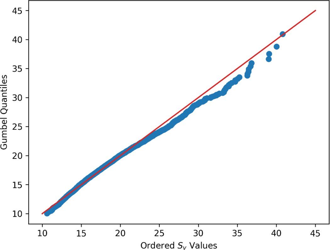
The Gumbel distribution is justified theoretically by taking the maximum of a collection of random variables and it becomes more tenable as the size of the collection increases. For the calculation of , the maximum is determined over an FoV. As the size as the FoV increases, the Gumbel distribution should become more appropriate as a model for . This implies making the FoVs as large as possible. However, large FoVs take a lot of time to measure. Further, the crucial assumption for the theory of independent and identically distributed observations may not hold for large FoVs because of spatial structure in the image used to calculate . Lastly, the observed values must be statistically independent for the maximum likelihood procedure described above to be appropriate. Irrespective of the size of measurement region chosen, we recommend examining the fit of the Gumbel distribution to the observed values. A histogram of the values with the fitted Gumbel probability density function overlaid, as shown in Figure 6, is one way to perform this validation. For smaller sample sizes, a quantile-quantile plot is more appropriate. A quantile-quantile plot shows the ordered observations on one axis versus the corresponding quantiles of the Gumbel distribution on the other. Such a plot is shown in Figure 7, using the same data depicted in both Figures 4 and 5. In the case that the Gumbel distribution accurately captures the observations, the ordered observations and quantiles should nearly follow a one-to-one relationship (denoted by the 45° line in Figure 6).
Figure 7.
Quantile-Quantile plot of values in the FoV dataset and fitted Gumbel distribution.
Return Value of for the Entire Surface from a Sample
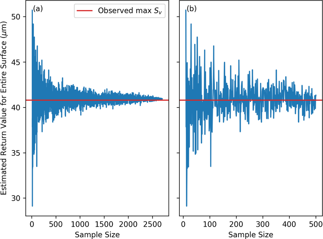
In most cases, we will not measure the surface of the entire part; instead, a small sample of FoVs will be measured. By fitting a Gumbel distribution to that sample, the return value for the whole part can be estimated. To investigate the performance of this approach, sample sizes from 10 to 2704 were chosen from the FoV dataset taken with the objective at random. Note that 2704 is the upper limit for the sample size as that is all the available values for a FoV with the objective as shown in Table 2. The return value of for the whole part was then calculated from the Gumbel distribution using the estimated values of and . The results of those calculations are shown in Figure 8. As expected, the accuracy of the prediction improves as the number of samples increases by converging to a value close to the observed maximum value (the horizontal red line). Note that the return values presented in Figure 8 do not include uncertainty or standard deviation from multiple iterations as those topics are covered later in the paper.
Figure 8.
Return values of for the entire part predicted from the Gumbel distribution, which was fit to a set of random samples from the full dataset. Subfigure a) shows the full set of calculations and subfigure b) shows sample sizes up to 500.
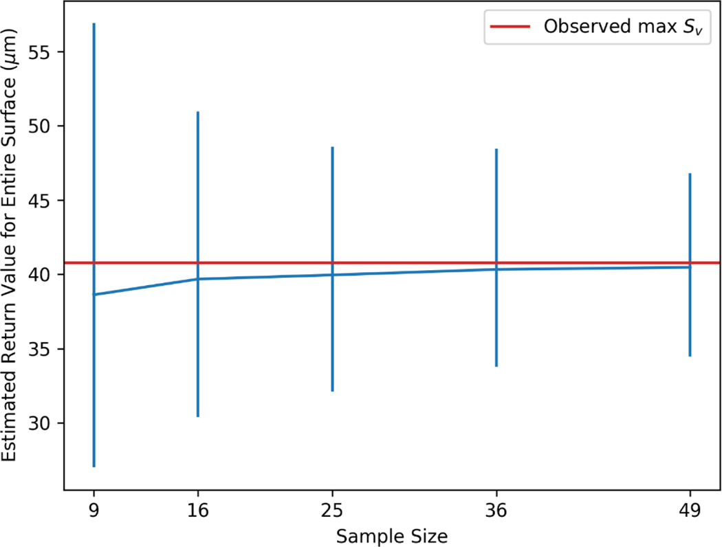
Moreover, we can investigate the repeated performance of a set of random samples. To achieve this, sets of 9, 16, 25, 36, and 49 values were randomly selected from the 2704 available values and fit with the Gumbel distribution to estimate the return value for the entire surface. This process was repeated 1000 times to provide a better understanding of the distribution of return values given a specific number of randomly selected values. The results of this analysis are shown in Figure 9.
Figure 9.
Median return values of for the entire part surface, calculated from the Gumbel distribution, which was fit to 9, 16, 25, 36, and 49 randomly selected values. Error bars represent the 2.5th and 97.5th quantiles from repeating this process for 1000 iterations.
Figure 9 shows the 2.5th and 97.5th quantiles of the 1000 repetitions (vertical blue lines) as well as the median (horizontal blue line). The observed maximum = 40.8 μm is depicted by the red line. As expected, the difference between the median return value and the actual maximum value of , as well as the spread in return values decreases as the number of randomly selected values increases. The largest decrease in the spread occurs between from 9 and 25 randomly selected measurements. This provides insight into the measurement routines that should be used in the inspection of large AM surfaces.
Uncertainty from a Single Sample
The intervals (vertical blue lines) in Figure 9 depict uncertainty due to sampling variability. To calculate the intervals in that figure, we were able to sample multiple times from our population of interest. However, in practice, sampling multiple times from our population of interest is not possible. Only a single sample of FoVs will be used to estimate the return value for the part surface. Maximum likelihood provides a strategy for assessing uncertainty with only a single sample. The negative inverse of the matrix of second derivatives of the log-likelihood function, evaluated at the maximum likelihood estimate, serves as an estimate of the variance-covariance matrix for and . This matrix is sometimes referred to as the observed information matrix. Since a return value for the Gumbel distribution is a linear combination of and , an estimate of the variance of the return value is a quadratic form of the observed information matrix. If the observed information matrix is denoted , then the standard error of the -FoV return value is
| (3) |
An approximate 95% confidence interval is then the canonical, estimate +/− twice the standard error.
Effect of Measurement Region Size
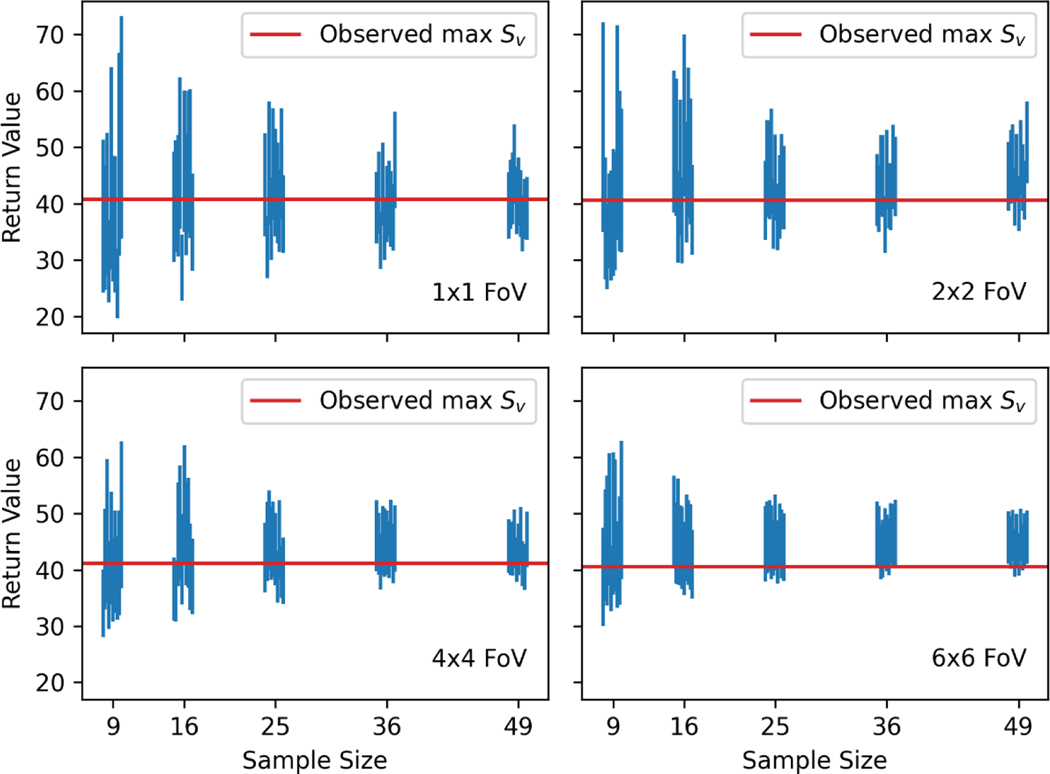
We can investigate the effect of the measurement region size on the prediction of . Figure 10 shows approximate 95% confidence intervals for the return value of the whole part surface for 20 combinations of sample size and measurement region size. Each combination is repeated 10 times. As expected, the widest intervals occur for the smallest combination of sample size and measurement region size, and the narrowest intervals occur for the largest combination of sample size and measurement region size. However, at the largest sample size, the intervals for the FoV size are very similar in width to the intervals for the FoV size at the largest sample size. In Figure 10, we also see a potential bias for the high sample size and high measurement region size combination. The confidence intervals almost all lie above the true maximum value of . For the pictured intervals, at the highest sample size (49 FoVs), the estimated bias for the FoV size is 0.3 μm, and for the FoV size it is 4.2 μm. We observe that the FoV data are not fitted very well by the Gumbel distribution (not pictured), leading to the biased results. This highlights the importance of examining the fit of the Gumbel distribution to the data, irrespective of the measurement region size. If the data and probability model do not match well, predictions from the probability are untrustworthy. Based on Figure 10, we recommend sampling as many small FoVs as resources permit, as long as the FoVs are large enough so that the Gumbel distribution provides a good fit to the sampled values.
Figure 10.
Approximate 95% confidence intervals for the return value of for the entire part surface for different combinations of sample size and FoV size. The individual vertical lines represent replicates from different random samples (10 each).
Limitations of the Study
Sampling Strategies
There are many sensible strategies to sample the surface of an AM part. In this paper we have focused only on sampling FoVs of various sizes at random. This is often a reasonable approach and can be easy to implement. However, it does not recognize the potential existence of spatial correlation between the values. A sampling strategy that intentionally distributes the samples over the whole surface may be more appropriate. One example is stratified sampling. In the current set up, an example of stratified sampling would be to sample completely at random one FoV from each FoV. We also might consider a 2D version systematic sampling. Since our surface is rectangular, an initial location is chosen at random in the upper left corner. Then the sampling is performed by rastering from left to right, and top to bottom by fixed horizontal and vertical displacements. This approach, however, requires a strong understanding of the longer spatial wavelengths that may affect the parameters being estimated as inadvertent matching of the sample spacing to those spatial wavelengths may lead to inaccurate results. Yet a third possibility is sampling according to a Latin Square design (depicted in Chapter 4 of Box et al., 2005) [47]. The most important point is that our samples are not clustered together with large portions of the surface left unsampled.
A strategy that we do not recommend is to separate measurements into smaller sets to increase the number of values for fitting. For example, assume five locations on the surface are chosen at random for measurement and a FoV stitched measurement is performed at each location. That would create five values of (i.e., one for each location). These five regions should not be divided into smaller ones to create more values for fitting the Gumbel distribution. If there exists spatial correlation between the values, this sampling strategy would invalidate the maximum likelihood approach to fitting and uncertainty quantification that we recommend. Consider this analogy. Suppose that we are estimating the return value of for the whole contiguous United States. If our sample was formed only by partitioning the state of Kansas, we would have a very biased view of the topography under study.
Measurement Uncertainty
While uncertainty due to the sampling and fitting of data is discussed in the previous section, it is also important to discuss the measurement uncertainty. Ideally, uncertainty with the measurand should be calculated based on the metrological characteristics of the equipment (e.g., those described in ISO 25178–600 [48]). However, this is a difficult and open problem that has yet to be solved for FV microscopy [34]. Additionally, uncertainty in the measurements affects the approach for fitting a Gumbel distribution to the data for prediction of extreme value parameters. There are several ways to include measurement uncertainty in the fitting procedure. One approach is to consider the measurements to be interval censored and use the fitting techniques described in Liu et al. [49]. Another is to use a measurement error model, which are common for calibration [50]. A last approach, which directly applies the fitting method described herein, is to perturb the measurements according to their uncertainties, fit a Gumbel distribution, and repeat in a Monte Carlo fashion. Regardless, uncertainty in the measurement of AM surfaces and proper application of that uncertainty to the measurand is an open and important topic for future work.
Conclusions
Part function can depend on the maximum value of a measurement parameter like . When we select a subset of our surface for measurement, we may or may not have the maximum value of the entire surface within our sample of FoVs. As researchers begin to find relationships between function and the maximum value of surface measurement parameters like (e.g., relationships between and fatigue cycles to failure [14]), it will become increasingly important to understand how to optimize measurement routines to estimate these peak values. This work has shown that a Gumbel distribution can be used for prediction of the maximum , for a large planar surface manufactured by laser powder bed fusion in IN625 using only a small subset of the surface. We found that 25 randomly selected FoVs balanced the tradeoffs between accuracy, uncertainty, and cost. In analysis of the effect of the number of randomly selected FoVs, the greatest decrease in the spread of the predicted maximum occurred between the selections of 9 to 25 FoVs. In analysis of the 95% confidence intervals for the FoV size, the average width of the intervals is 16 μm for 25 randomly selected FoVs, and 12 μm for 49 randomly selected FoVs. In addition, for large FoV sizes (e.g., the FoV size), a bias is observed in the results. For 49 randomly selected FoVs, the estimated bias is 4.2 μm. This tradeoff, however, will be dependent on the application and how critical the inspection is to the use of the part. For example, flight critical components will require greater confidence in the result of the inspection than non-flight critical ones.
While these methods provide a strong basis for the development of measurement routines for inspection and quality assurance, they will work best when the surface topography under study is mostly homogeneous. They are unlikely to predict events that are independent of the AM process (e.g., a scratch on the optics which interferes with the laser, damage from handling the surface with improper tools, etc.). Thus, as users investigate the relationship between surface structures and function and develop sampling routines in order to determine quality of the part, this method should not be used for defect detection. Other probabilistic models and sampling strategies would be necessary to achieve that goal. It is likely that much larger sample sizes would be necessary to provide a high degree of confidence that a part is defect free.
Additionally, the design of the part in this study minimized variability (i.e., a single large planar part near the center of the build volume, with no change in dwell time due variable sizes of neighboring parts for a given layer). In a system where complexity is a hallmark of parts produced, it will be important to test how correlations between part function and surface topography parameters like hold as additional variables are introduced. These variables may include, but are not limited to, changes in geometry, positioning, process parameters, post-processing, feedstock condition, and build environment. Future work should take these factors into account to better determine the applicability of the Gumbel distribution for the prediction of peak surface topography parameters like .
Acknowledgements
The authors would like to thank Dr. John S. Taylor and Dr. Christopher Evans for their insightful comments on surface characterization and how these methods may/may not apply to defect detection. The authors would also like to thank Dr. Christopher Evans and the students of his Advanced Surface Metrology course at the University of North Carolina at Charlotte for their astute questions and discussion following a presentation of this work, which allowed us to better prepare and describe the information contained in this manuscript.
Appendix: Python Code for Gumbel Distribution Fit
full_histogram.py:

import pandas as pd
import numpy as np

import matplotlib
import matplotlib.pyplot as plt
import gumbel_mle

fovs = pd.read_csv(“./20x_1×1_0p0022to0p405.csv”, header=None, skiprows=2)
fovs = fovs.iloc[:, 14]

mle, vcov = gumbel_mle.gumbel_mle(fovs)


def gumbel_pdf(mu, sigma, x):
   z = (x - mu)/sigma
   return (1/sigma)*np.exp(−(z + np.exp(−z)))


x = np.linspace(10, 45, 100)
fx = gumbel_pdf(mle[0], mle[1], x)

plt.hist(fovs, density=True)
for i in range(50):
   mle_str = np.random.multivariate_normal(mle, vcov)
   fx_str = gumbel_pdf(mle_str[0], mle_str[1], x)
   plt.plot(x, fx_str, color = “tab:red”,
	    alpha = 0.05)
plt.plot(x, fx, color=“tab:red”,
	    label=“Gumbel Distribution”)
plt.xlabel(“$S_v$ ($\mu$m)”)
plt.ylabel(“Density”)
plt.legend()
ax = plt.gca()
ax.spines[‘top’].set_visible(False)
ax.spines[‘right’].set_visible(False)
plt.savefig(“hist_density_1×1_fovs.png”, dpi=300)
plt.close(“all”)


def gumbel_inv_cdf(mu, sigma, p):
    return mu - sigma*np.log(-np.log(p))

n = fovs.shape[0]
p = np.linspace(1/n, (n - 1)/n, n)

plt.plot(np.sort(fovs),
	 gumbel_inv_cdf(mle[0], mle[1], p),
	 “o”)
plt.plot([10, 45], [10, 45], color=“tab:red”)
plt.xlabel(“Ordered $S_v$ Values”)
plt.ylabel(“Gumbel Quantiles”)
plt.savefig(“full_quantile-quantile_1×1_fovs.png”, dpi=300)

Gumble_mle.py:

import numpy as np
import scipy.optimize

def ll(theta, x):
   mu = theta[0]
   lbeta = theta[1]
   beta = np.exp(lbeta)
   n = len(x)

   term1 = n*lbeta
   term2 = (1/beta)*(np.sum(x) - n*mu)
   term3 = np.sum(np.exp((mu - x)/beta))

   return term1+term2+term3


def gumbel_mle(x):
   beta_hat = np.sqrt(6)/np.pi*np.std(x)
   mu_hat = np.mean(x) - beta_hat*np.euler_gamma
   lbeta_hat = np.log(beta_hat)


   mle = scipy.optimize.minimize(ll, np.array([mu_hat, lbeta_hat]),
		  args=(x))
   tmp = mle.x.copy()
   mle_est = np.array([tmp[0], np.exp(tmp[1])])

   tmp = mle.hess_inv.copy()
   mle_vcov = np.array([[tmp[0, 0], tmp[0, 1]*mle_est[1]],
	     [tmp[0, 1]*mle_est[1], tmp[1, 1]*mle_est[1]**2]])
   return mle_est, mle_vcov


def gumbel_return_value(x, N):

   mle_est, mle_vcov = gumbel_mle(x)
   mu = mle_est[0]
   beta = mle_est[1]

   return_value = mu - beta*np.log(np.log(N) - np.log(N - 1))

   gradient = np.array([[1, -np.log(np.log(N) - np.log(N - 1))]])

   return_value_se = np.sqrt((gradient @ mle_vcov @ gradient.T)[0, 0])

   return return_value, return_value_se
Footnotes
Certain commercial entities, equipment, or materials may be identified in this document to describe an experimental procedure or concept adequately. Such identification is not intended to imply recommendation or endorsement by the National Institute of Standards and Technology, nor is it intended to imply that the entities, materials, or equipment are necessarily the best available for the purpose.
References
- [1].Gisario A, Kazarian M, Martina F, Mehrpouya M, Metal additive manufacturing in the commercial aviation industry: A review, J. Manuf. Syst 53 (2019) 124–149. 10.1016/j.jmsy.2019.08.005. [DOI] [Google Scholar]
- [2].Sobota VCM, van de Kaa G, Luomaranta T, Martinsuo M, Ortt JR, Factors for metal additive manufacturing technology selection, J. Manuf. Technol. Manag 32 (2020) 26–47. 10.1108/JMTM-12-2019-0448. [DOI] [Google Scholar]
- [3].Yadroitsev I, Selective laser melting: direct manufacturing of 3D-objects by selective laser melting of metal powders, Lambert Acad. Publ, Saarbrücken, 2009. [Google Scholar]
- [4].Measurement Science Roadmap for Metal-Based Additive Manufacturing, NIST, US Department of Commerce, 2012. [Google Scholar]
- [5].America Makes & ANSI Additive Manufacturing Standardization Collaborative Standardization Roadmap for Additive Manufacturing, Public Draft v2.0, (2018).
- [6].Townsend A, Senin N, Blunt L, Leach RK, Taylor JS, Surface texture metrology for metal additive manufacturing: a review, Precis. Eng 46 (2016) 34–47. 10.1016/j.precisioneng.2016.06.001. [DOI] [Google Scholar]
- [7].Leach RK, Bourell D, Carmignato S, Donmez A, Senin N, Dewulf W, Geometrical metrology for metal additive manufacturing, CIRP Ann. 68 (2019) 677–700. 10.1016/j.cirp.2019.05.004. [DOI] [Google Scholar]
- [8].Kleszczynski S, Ladewig A, Friedberger K, zur Jacobsmühlen J, Merhof D, Witt G, Position Dependency of Surface Roughness in Parts from Laser Beam Melting Systems, in: Proc. 26th Int. Solid Free. Fabr. SFF Symp., Austin, TX, 2015: pp. 360–370. [Google Scholar]
- [9].Rott S, Ladewig A, Friedberger K, Casper J, Full M, Schleifenbaum JH, Surface roughness in laser powder bed fusion – Interdependency of surface orientation and laser incidence, Addit. Manuf 36 (2020) 101437. 10.1016/j.addma.2020.101437. [DOI] [Google Scholar]
- [10].Fox JC, Moylan SP, Lane BM, Effect of Process Parameters on the Surface Roughness of Overhanging Structures in Laser Powder Bed Fusion Additive Manufacturing, in: Procedia CIRP, Charlotte, NC, 2016: pp. 131–134. 10.1016/j.procir.2016.02.347. [DOI] [Google Scholar]
- [11].Fox JC, Moylan S, Lane BM, Preliminary Study Toward Surface Texture as a Process Signature in Laser Powder Bed Fusion Additive Manufacturing, in: Proc. 2016 ASPE Summer Top. Meet. Dimens. Accuracy Surf. Finish Addit. Manuf., Raleigh, NC, 2016. [Google Scholar]
- [12].Triantaphyllou A, Giusca CL, Macaulay GD, Roerig F, Hoebel M, Leach RK, Tomita B, Milne KA, Surface texture measurement for additive manufacturing, Surf. Topogr. Metrol. Prop 3 (2015) 024002. 10.1088/2051-672X/3/2/024002. [DOI] [Google Scholar]
- [13].Stimpson CK, Snyder JC, Thole KA, Mongillo D, Roughness Effects on Flow and Heat Transfer for Additively Manufactured Channels, J. Turbomach 138 (2016) 051008. 10.1115/1.4032167. [DOI] [Google Scholar]
- [14].Gockel J, Sheridan L, Koerper B, Whip B, The influence of additive manufacturing processing parameters on surface roughness and fatigue life, Int. J. Fatigue 124 (2019) 380–388. 10.1016/j.ijfatigue.2019.03.025. [DOI] [Google Scholar]
- [15].Zhang J, Fatemi A, Surface roughness effect on multiaxial fatigue behavior of additive manufactured metals and its modeling, Theor. Appl. Fract. Mech 103 (2019) 102260. 10.1016/j.tafmec.2019.102260. [DOI] [Google Scholar]
- [16].ASME B46.1: Surface Texture (Surface Roughness, Waviness, and Lay), New York, NY, (2019). [Google Scholar]
- [17].ISO 4287:1997 - Geometrical Product Specifications (GPS) – Surface texture: Profile method – Terms, definitions and surface texture parameters, ISO, Geneva, (1997). [Google Scholar]
- [18].ISO 25178–2:2012 - Geometrical Product Specifications (GPS) - Surface Texture: Areal - Part 2: Terms, definitions, and surface texture parameters, ISO, Geneva., (2012). [Google Scholar]
- [19].Senin N, Thompson A, Leach RK, Feature-based characterisation of signature topography in laser powder bed fusion of metals, Meas. Sci. Technol 29 (2017). 10.1088/1361-6501/aa9e19. [DOI] [Google Scholar]
- [20].Newton L, Senin N, Smith B, Chatzivagiannis E, Leach R, Comparison and validation of surface topography segmentation methods for feature-based characterisation of metal powder bed fusion surfaces, Surf. Topogr. Metrol. Prop 7 (2019) 045020. 10.1088/2051-672X/ab520a. [DOI] [Google Scholar]
- [21].Strano G, Hao L, Everson RM, Evans KE, Surface roughness analysis, modelling and prediction in selective laser melting, J. Mater. Process. Technol 213 (2013) 589–597. 10.1016/j.jmatprotec.2012.11.011. [DOI] [Google Scholar]
- [22].Cabanettes F, Joubert A, Chardon G, Dumas V, Rech J, Grosjean C, Dimkovski Z, Topography of as built surfaces generated in metal additive manufacturing: A multi scale analysis from form to roughness, Precis. Eng 52 (2018) 249–265. 10.1016/j.precisioneng.2018.01.002. [DOI] [Google Scholar]
- [23].Tian Y, Tomus D, Rometsch P, Wu X, Influences of processing parameters on surface roughness of Hastelloy X produced by selective laser melting, Addit. Manuf 13 (2017) 103–112. 10.1016/j.addma.2016.10.010. [DOI] [Google Scholar]
- [24].Leach R, Haitjema H, Bandwidth characteristics and comparisons of surface texture measuring instruments, Meas. Sci. Technol 21 (2010) 032001. 10.1088/0957-0233/21/3/032001. [DOI] [Google Scholar]
- [25].Thompson A, Senin N, Giusca C, Leach R, Topography of selectively laser melted surfaces: A comparison of different measurement methods, CIRP Ann. 66 (2017) 543–546. 10.1016/j.cirp.2017.04.075. [DOI] [Google Scholar]
- [26].Zanini F, Sbettega E, Sorgato M, Carmignato S, New Approach for Verifying the Accuracy of X-ray Computed Tomography Measurements of Surface Topographies in Additively Manufactured Metal Parts, J. Nondestruct. Eval 38 (2018) 12. 10.1007/s10921-018-0547-4. [DOI] [Google Scholar]
- [27].Zanini F, Pagani L, Savio E, Carmignato S, Characterisation of additively manufactured metal surfaces by means of X-ray computed tomography and generalised surface texture parameters, CIRP Ann. 68 (2019) 515–518. 10.1016/j.cirp.2019.04.074. [DOI] [Google Scholar]
- [28].Fox JC, Kim FH, Reese ZC, Evans C, Investigation of complementary use of optical metrology and x-ray computed tomography for surface finish in laser powder bed fusion additive manufacturing, in: Proc. Jt. Spec. Interest Group Meet. Euspen ASPE, Leuven, Belgium, 2017: pp. 132–136. [Google Scholar]
- [29].Fox JC, Kim FH, Reese ZC, Evans C, Complementary Use of Optical Metrology and X-Ray Computed Tomography for Surface Finish and Defect Detection in Laser Powder Bed Fusion Additive Manufacturing, in: Proc. 2018 ASPE Euspen Summer Top. Meet. - Adv. Precis. Addit. Manuf., Berkeley, CA, 2018: pp. 195–200. [Google Scholar]
- [30].Leach R, Senin N, Feng X, Stavroulakis P, Su R, Syam W, Widjanarko T, Information-rich metrology: Changing the game, (n.d.) 11. [Google Scholar]
- [31].Fox JC, Pintar A, Effect of measurement and sampling strategy in surface analysis of laser powder bed fusion additive manufacturing of nickel superalloy 625, in: Proc. 2019 Spec. Interest Group Meet. Adv. Precis. Addit. Manuf., Nantes, FR, 2019: p. 4. [Google Scholar]
- [32].Petzing J, Coupland J, Leach R, The Measurement of Rough Surface Topography using Coherence Scanning Interferometry, National Physical Laboratory, 2010.
- [33].Gomez C, Su R, Thompson A, DiSciacca J, Lawes S, Leach RK, Optimization of surface measurement for metal additive manufacturing using coherence scanning interferometry, Opt. Eng 56 (2017) 111714. 10.1117/1.OE.56.11.111714. [DOI] [Google Scholar]
- [34].Newton L, Senin N, Gomez C, Danzl R, Helmli F, Blunt L, Leach R, Areal topography measurement of metal additive surfaces using focus variation microscopy, Addit. Manuf 25 (2019) 365–389. 10.1016/j.addma.2018.11.013. [DOI] [Google Scholar]
- [35].WK66682 New Guide for Evaluating Post-processing and Characterization Techniques for AM Part Surfaces, (n.d.). https://www.astm.org/DATABASE.CART/WORKITEMS/WK66682.htm (accessed May 11, 2020).
- [36].Material Data Sheet - EOS NickelAlloy IN625, (2011). http://ip-saas-eos-cms.s3.amazonaws.com/public/d1327facdca0e32a/373a60ec4f5c891b7dbcdf572e37d3b0/EOS_NickelAlloy_IN625_en.pdf (accessed June 13, 2017).
- [37].ISO 25178–606:2015, Geometrical product specification (GPS) -- Surface texture: Areal -- Part 606: Nominal characteristics of non-contact (focus variation) instruments, (2015).
- [38].Alicona, Technical Specifications of the Alicona InfiniteFocus, Alicona Focus Var. English Edition 6 (2016). https://www.alicona.com/en/products/infinitefocus/ (accessed December 20, 2016). [Google Scholar]
- [39].OpenFMC X3P Support Library, The OpenFMC Repository for C/C++ and Other Code for Reading and Writing X3P Files, 2016. https://github.com/OpenFMC/x3p (accessed September 26, 2018).
- [40].OmniSurf3D, v1.02.002, Digital Metrology Solutions, Inc, 2019. https://digitalmetrology.com/.
- [41].ISO 25178–3:2012 - Geometrical Product Specifications (GPS) - Surface Texture: Areal - Part 3: Specification operators, ISO, Geneva., (2012). [Google Scholar]
- [42].Fisher RA, Tippett LHC, Limiting forms of the frequency distribution of the largest or smallest member of a sample, in: Math. Proc. Camb. Philos. Soc, Cambridge University Press, 1928: pp. 180–190. [Google Scholar]
- [43].NIST, Digital Library of Mathematical Functions: Section 5.2 (II) Euler’s Constant, (2020). https://dlmf.nist.gov/5.2 (accessed December 30, 2020).
- [44].Casella G, Berger RL, Statistical Inference, Thomson Learning, 2002.
- [45].Thomas M, Su R, de Groot P, Leach R, Optical topography measurement of steeply-sloped surfaces beyond the specular numerical aperture limit, in: Opt. Photonics Adv. Dimens. Metrol., International Society for Optics and Photonics, 2020: p. 1135207. 10.1117/12.2554568. [DOI]
- [46].Danzl R, Helmli F, Scherer S, Focus Variation – a Robust Technology for High Resolution Optical 3D Surface Metrology, Stroj. Vestn. – J. Mech. Eng 2011 (2011) 245–256. 10.5545/sv-jme.2010.175. [DOI] [Google Scholar]
- [47].Box GE, Hunter JS, Hunter WG, Statistics for Experimenters: Design, Innovation, and Discovery, 2nd ed., Wiley-Interscience, Hoboken, 2005. [Google Scholar]
- [48].ISO 25178–600:2019 - Geometrical Product Specifications (GPS) - Surface Texture: Areal - Part 600: Mettrological characteristics for areal topography measuring methods, ISO, Geneva., (2019). [Google Scholar]
- [49].Liu S, Wu H, Meeker WQ, Understanding and Addressing the Unbounded “Likelihood” Problem, Am. Stat 69 (2015) 191–200. 10.1080/00031305.2014.1003968. [DOI] [Google Scholar]
- [50].Carroll RJ, Ruppert D, Stefanski LA, Crainiceanu CM, Measurement Error in Nonlinear Models: A Modern Perspective, Second Edition, CRC Press, 2006. [Google Scholar]


