Coexistence of populations in a Leslie-Gower tritrophic model with Holling-type functional responses

Abstract

The dynamics of a Leslie-Gower type tritrophic model are analyzed. The model considers the interaction among three populations, a resource, a predator and a superpredator. It is assumed that the predator is generalist and its interaction with the resource is according to a general Holling-type functional response. Furthermore, it is assumed that the superpredator is specialist and its interaction with the predator follows a Holling type II functional response. The goal of this work is to show conditions that guarantee the coexistence of the three species. To do this, the existence of a stable equilibrium point or a stable limit cycle is demonstrated, which appears via a bifurcation. In addition, the analytical results are exemplified through numerical simulations.

1. Introduction

The growing relevance of the mathematical modeling is due, in a significant way, to the fact that it allows us to get theoretical knowledge consistent with a variety of observable behaviors in nature. Among the characteristics that are considered in the modeling, there are reproduction rates, mortality rates, alternative resource for the predator, defense mechanisms of the prey and the intraspecific and interspecific competition. On the other hand, one of the topics of population ecology where mathematical methods are most frequently applied is the predator-prey interaction; in particular, intraguild predation is a field that presents interesting challenges for researchers, both from a mathematical and theoretical ecological point of view. Seo and Kot [14] studied a system with two predators assuming that top predator is a generalist whose population is in equilibrium; taking the population of the top predator as a bifurcation parameter they depict a rich dynamics of the system that includes the existence of simultaneous limit cycles. They find evidence that the generalist predator favors stability in a system whose fluctuations are caused by the specialist mesopredator. Recently in [4] the authors considered a tritrophic model with linear or logistic growth function for the prey population, a functional response Holling III type for predator and a functional response Holling IV type for superpredator. The authors proved that there is a stable limit cycle arising from a Bautin bifurcation. In [17] the authors consider the case developed by [4] and prove the existence of three limit cycles around the coexistence equilibrium point, emerging from a Hopf bifurcation.

One of the classic models in the literature is the Leslie-Gower predator-prey model, see [11], given by the following equations,

$$\dot{x}=xR(x)-f(x)y,\dot{y}=sy(1-\frac{y}{nx}).$$

Where $x(t)$ and $y(t)$ denote the density of prey and predator at time t, respectively. The function $xR(x)$ is the prey growth rate and $f(x)$ is the functional response. The parameter s is the predator growth rate and the predator benefits from the prey in its carrying capacity are nx. In population dynamics Leslie-Gower type models have played an important role in mathematical modeling from 1960 to the present see [3], [7], [13]. Predators can be divided into two groups: specialists and generalists see [6], [14], [15]. The study of tritrophic species in a food web for a generalist-specialist-prey system offers a rich and complex dynamic [8], [13]; in fact, Haski et al. [6] suggests that specialist predators contribute to population cycles and generalist predators with a stabilizing contribution.

Recently in [4] the authors considered a tritrophic model with linear or logistic growth function for the prey population, a functional response Holling III type for predator and a functional response Holling IV type for superpredator. In [4] they proved that there is a stable limit cycle at the corresponding coexistence equilibrium point. In [17] the authors consider the case developed by [4] and prove the existence of three limit cycles around the coexistence equilibrium point, emerging from a Hopf bifurcation.

Based on this predator prey system, in this work a tritrophic food chain is modeled by the following system of three differential equations,

$$\dot{x}=rx(1-\frac{x}{K})-\frac{qxy}{x^m+a},\dot{y}=\alpha y(1-\frac{y}{nx+c})-\frac{q_{1}yz}{z+b},\dot{z}=\mu \frac{q_{1}yz}{z+b}-dz.$$ (1)

Where $x(t)$, $y(t)$ and $z(t)$ stand for the population density of the prey, generalist predator and specialist superpredator, respectively. All the parameters r, K, q, m, a, α, n, c, $q_1$, b, μ and d are positive. A generalist predator $y(t)$ has the characteristic of having an ecological niche with wide potential, on the contrary a specialist superpredator $z(t)$ feeds on a single species or a few, thus its potential niche is small. One of the novel features of system (1) is that only a proportion $q_1$ of the prey population y is susceptible to being preyed on by the superpredator z; This happens, for example, when the predator specializes on a certain group (size, age, etc.) of the prey population. As z increases, the prey population decreases, not exceeding $q_{1}y$. We consider in (1) that the prey population has a logistic growth and $F(x)=\frac{qx}{x^m+a}$ is a generalization of the Holling type functional response. The functional response $F(x)$, for $m>1$ represents a defense mechanism of the prey, see [16].

The coexistence of the three populations, through a stable coexistence equilibrium point or a stable periodic orbit is analyzed. In particular, the existence of periodic orbits that arise through Hopf or Bautin bifurcations is determined.

System (1) constrained to prey x and predator y was studied in [16]; for $m=2$ the authors determine a region in the parameter space where there are supercritical Hopf bifurcations or Bautin bifurcation. In addition, the existence of simultaneous Hopf bifurcations is demonstrated. The system (1) with a logistic growth prey and a general functional response is analyzed in [1]. The authors studied a predator prey model with two generalist predators and proved the existence of a Bogdanov-Takens bifurcation. In [2], the authors give conditions to have a stable limit cycle obtained by an Andronov-Hopf bifurcation in a Gause tritrophic model. They consider a generalized logistic growth function for the prey, and a general family of functional responses.

In this paper, we analyze the local dynamics of Leslie-Gower type tritrophic model (1), which considers the interaction among three populations, a resource, a predator and a superpredator. The goal of this work is to show conditions that guarantee the coexistence of the three species. For this, we show the existence of a stable equilibrium point or a stable limit cycle, which appears via a bifurcation. In particular, we prove that system (1) exhibits a Bautin bifurcation and consequently there are bistability given by a stable equilibrium point and a stable periodic orbit.

In Section 2, we give necessary and sufficient parameter conditions to have coexistence equilibrium points. Section 3 is devoted to prove main Theorem 3.1, which guarantee sufficient parameter conditions to have an equilibrium point where differential system (1) exhibits a Bautin bifurcation. In Section 4, we give numerical simulations to exemplify the analytical results.

2. Equilibrium points in the positive octant

Proposition 2.1

The solutions of system (1) are non-negative and bounded for all $t\ge 0$ .

Proof

Since the planes $x=0,y=0$ and $z=0$, are invariant the solutions of system (1) with initial conditions $(x_0,y_0,z_0)$ in the positive octant remain in it and are positive for all t.

We will do the analysis to prove that $(x(t),y(t),z(t))$ is bounded for all $t\ge 0$.

From the differential inequality

$$\dot{x}=rx(1-\frac{x}{K})-\frac{qxy}{x^m+a}\le rx(1-\frac{x}{K}),$$

it follows that $\underset{t\to \infty }{\lim }\text{sup }x(t)\le K$. Then, given $ϵ>0$ there exists $T>0$, such that

$$x(t)<K+\frac{ϵ}{2},$$

for all $t>T$. Therefore,

$$\dot{y}=\alpha y(1-\frac{y}{nx+c})-\frac{q_{1}yz}{z+b}\le \alpha y(1-\frac{y}{nx+c})\le \alpha y(1-\frac{y}{n(K+\frac{ϵ}{2})+c}),$$

which implies that $\underset{t\to \infty }{\lim }\text{sup }y(t)\le n(K+\frac{ϵ}{2})+c$. Then,

$$\underset{t\to \infty }{\lim }\text{sup }y(t)\le nK+c,$$ (2)

since ϵ is arbitrary. Finally,

$$\dot{z}=\mu q_{1}y\left(\frac{z}{z+b}\right)-dz\le \mu q_{1}y-dz.$$ (3)

From (2) and (3) it follows that

$$\dot{z}\le \mu q_1(nK+c)-dz,$$

then

$$\underset{t\to \infty }{\lim }\text{sup }z(t)\le \frac{\mu q_1(nK+c)}{d}.$$

Thus, $x(t)$, $y(t)$ and $z(t)$ are bounded for $t\ge 0$ and are non-negative.

For ecological considerations, the region of interest in ${\mathbb{R}}^3$ is the positive octant $\mathrm{\Omega }=\{(x,y,z)\in {\mathbb{R}}^3:x>0,y>0,z>0\}$.

The following lemma guarantees the existence of at least an equilibrium point of the system (1) in the region of interest.

Lemma 2.1

Assume that all parameters of the system(1)are positive. The point$P^{⁎}=(x_0,y_0,z_0)\in \mathrm{\Omega }$is an equilibrium of system(1)if and only if the parameters q, μ and the second coordinate of$P^{⁎}$satisfy

$$q=\frac{r(K-x_0)(a+x_0^m)(b+z_0)\alpha }{K(c+n{x}_0)(\alpha (b+z_0)-q_1{z}_0)}\mathit{\text{,}}\mu =\frac{d{(b+z_0)}^2\alpha }{q_1(c+n{x}_0)(\alpha (b+z_0)-q_1{z}_0)},$$

$$y_0=\frac{(c+n{x}_0)(\alpha (b+z_0)-q_1{z}_0)}{(b+z_0)\alpha }\mathit{\text{,}}\alpha (b+z_0)>q_1{z}_0\mathit{\text{and}}K>x_0.$$ (4)

Proof

In order to find an equilibrium point for the system (1) we need to find the solutions of the following system of equations:

$$0=x(r(1-\frac{x}{K})-\frac{qy}{x^m+a}),0=y(\alpha (1-\frac{y}{nx+c})-\frac{q_{1}z}{z+b}),0=z(\mu \frac{q_{1}y}{z+b}-d).$$ (5)

In order to solve the above system, we multiply the first equation of (5) for $K(x^m+a)$.

$$0=x((x^m+a)r(K-x)-Kqy),0=y(\alpha (1-\frac{y}{nx+c})-\frac{q_{1}z}{z+b}),0=z(\mu \frac{q_{1}y}{z+b}-d).$$

The point $(x_0,y_0,z_0)\in \mathrm{\Omega }$ is an equilibrium point of the system (1) if and only if $(x_0,y_0,z_0)$ is a positive solution of

$$(x^m+a)r(K-x)-Kqy=0,\alpha (1-\frac{y}{nx+c})-\frac{q_{1}z}{z+b}=0,\mu \frac{q_{1}y}{z+b}-d=0.$$ (6)

Solving in $y_0$ the second and third equation of system (6) we obtain

$$y_0=\frac{(c+n{x}_0)(\alpha (b+z_0)-q_1{z}_0)}{(b+z_0)\alpha }$$ (7)

and

$$y_0=\frac{d(b+z_0)}{q_1\mu }.$$ (8)

Equaling (7) and (8) and solving for μ we obtain

$$\mu =\frac{d{(b+z_0)}^2\alpha }{q_1(c+n{x}_0)(\alpha (b+z_0)-q_1{z}_0)}.$$

Since q is linear in the first equation of system (6), we solve it in terms of q and obtain

$$q=\frac{r(K-x_0)(a+x_0^m)(b+z_0)\alpha }{K(c+n{x}_0)(\alpha (b+z_0)-q_1{z}_0)}.$$

Hence, $P^{⁎}=(x_0,y_0,z_0)\in \mathrm{\Omega }$ if and only if q, μ and $y_0$ satisfy (4).

Remark 2.1

If condition(4)inLemma 2.1is satisfied and

$$\alpha =\frac{s_1+q_1{z}_0}{b+z_0}\mathit{\text{with}}{s}_1>0,$$

then$P^{⁎}=(x_0,\frac{s_1(c+n{x}_0)}{s_1+q_1{z}_0},z_0)$ ∈Ω.

Remark 2.2

System (1) has at most three equilibrium points in the first octant.

Substituting (7) in the first equation (6) , we have the following polinomial

$$P(x)=-r_1\alpha (b+z_0)x^{m+2}+K{r}_1\alpha (b+z_0)x^{m+1}+[Knq(q_1{z}_0-(b+z_0)\alpha )-a{r}_1\alpha (b+z_0)]x^2+K[cq(q_1{z}_0-(b+z_0)\alpha )+a{r}_1\alpha (b+z_0)]x.$$

In order to determine the number of points in the positive octant, we apply Descartes' rule of signs to $P(x)$ . Since $y_0>0$ , from (4) we have that $\alpha (b+z_0)>q_1{z}_0$ , consequently the coefficient of the quadratic term is negative. For the coefficient of the linear term, we have two cases:

• •
  If

  $$a{r}_1\alpha (b+z_0)>|cq(q_1{z}_0-(b+z_0)\alpha |.$$

  The coefficient is positive and $P(x)$ has three changes of sign. Therefore $P(x)$ has three or one positive roots.
• •
  If

  $$a{r}_1\alpha (b+z_0)<|cq(q_1{z}_0-(b+z_0)\alpha |.$$

  The coefficient is negative and $P(x)$ has two changes of sign. Therefore $P(x)$ has two or zero positive roots.

Hence, we can conclude that system (1) can have at most three equilibrium points in the first octant.

3. Hopf and Bautin bifurcation at equilibrium point $P_0$

In order to simplify the expressions we fixed the parameters $m=2$, $x_0=1,z_0=1$, $n=1,q_1=1$ and $b=1$. From Lemma 2.1 we have

$$q=\frac{2(1+a)(K-1)r\alpha }{(1+c)K(2\alpha -1)}\text{ and }\mu =\frac{4d\alpha }{(1+c)(2\alpha -1)}\text{ with }2\alpha >1\text{ and }K>1.$$

Then system (1) has the following equilibrium point in the first octant

$$P_0(c,\alpha )=(1,\frac{(1+c)(2\alpha -1)}{2\alpha },1).$$

In order to show conditions to have a Hopf or Bautin bifurcation, we define the following parameters.

$$\begin{gathered} a_0=\frac{K(8+3d^2-d^3+4d(-1+r))-6dr)}{(-8+4d-3d^2+d^3)K+2dr},c_0=-(d(-8+6d-4d^2+d^3)r+K(64-7d^5+d^6+d^4(23-2r)-12d^2(r-7)+16d(-5+r)+d^3(-53+8r)))/((4-d+d^2)(16-16d+13d^2-6d^3+d^4)K)\text{ and } \\ {\alpha }_0=\frac{7-\frac{8}{d}-4d+d^2}{2}. \end{gathered}$$ (9)

We denote by $J(x,y,z)$ the Jacobian matrix associate to vector field (1).

Lemma 3.1

If $a=a_0$ , $c=c_0$ and $\alpha ={\alpha }_0$ in system (1) then the eigenvalues of $J(P_0(c_0,{\alpha }_0))$ are

$${\lambda }_{1,2}=\pm i\mathit{\text{and}}{\lambda }_3=-1.$$

Proof

The characteristic polynomial of $J(P_0(c,\alpha ))$ is:

$$p(\lambda )=-\frac{dr(1+a+4\alpha +6c\alpha +2ac\alpha +aK(2\alpha -1)-K(1+(2+4c)\alpha ))}{4(1+a)(1+c)K}+(-\frac{d\alpha }{2}-\frac{r(d(3+a-2K)+(2+(-1+a)K)(2\alpha -1)}{2(1+a)(1+c)K}+\frac{c(3+a-2K)(-1+d+2\alpha ))}{2(1+a)(1+c)K})\lambda +(\frac{1}{2}-\frac{d}{2}-\frac{(3+a-2K)r}{(1+a)K}-\alpha ){\lambda }^2-{\lambda }^3.$$

Taking $a=a_0$, $c=c_0$ and $\alpha ={\alpha }_0$

$$p(\lambda )=-(1+\lambda )({\lambda }^2+1).$$

Then, the eigenvalues of $J(P_0(c_0,{\alpha }_0))$ are

$${\lambda }_{1,2}=\pm i\text{ and }{\lambda }_3=-1.$$

Proposition 3.1

If the hypotheses of Lemma 3.1 are satisfied, then there exists a three-dimensional manifold $\mathcal{L}$ in the parameter space $d-r-K$ , such that the eigenvalues of $J(P_0(c_0,{\alpha }_0))$ are ${\lambda }_{1,2}=\pm i,{\lambda }_3=-1$ , and the first Lyapunov coefficient is equal to zero for all $(d,r,K)\in \mathcal{L}$ .

Proof

By Lemma 3.1, the eigenvalues of $J(P_0(c_0,{\alpha }_0))$ are ${\lambda }_{1,2}=\pm i,{\lambda }_3=-1$. In order to calculate the first Lyapunov coefficient ${\ell }_1$, we use the Kuznetsov's formula (see Appendix A.1).

Moving $P_0(c_0,{\alpha }_0)$ to origin we obtain the next equivalent system,

$$\dot{x}=rx(1-\frac{x}{K}-\frac{R_1}{R_2}),\dot{y}=\frac{1}{2}(7-\frac{8}{d}-4d+d^2)y(1-\frac{y}{R_3})-\frac{yz}{1+z},\dot{z}=-dz+\frac{R_4}{{(-8+6d-4d^2+d^3)}^2(K-1)r(1+z)},$$ (10)

where

$$R_1=2(4-d+d^2)(-8+7d-4d^2+d^3)(16-16d+13d^2-6d^3+d^4)(K-1)y,R_2={(-8+6d-4d^2+d^3)}^2(2dr(-3+x^2)+K(8-8x^2-3d^2(-1+x^2)+d^3(-1+x^2)+4d(-1+r+x^2))),R_3=-(2d(-8+6d-4d^2+d^3)r+K(64-7d^5+d^6+d^4(23-2r)-12d^2(-7+r)+16d(-5+r)+d^3(-53+8r)))/((4-d+d^2)(16-16d+13d^2-6d^3+d^4)K).R_4=(4-d+d^2)(-8+7d-4d^2+d^3)(16-16d+13d^2-6d^3+d^4)Kyz.$$

Let A the Jacobian matrix of system (10) evaluate at zero (see Appendix A.2). The bilinear and trilinear forms B and C at the equilibrium $p=(0,0,0)$ are given in Appendix A.3. The eigenvectors of A are

$${\mathbf{\text{v}}}_1=(v_1,v_2,1),{\mathbf{\text{v}}}_2={\overline{\mathbf{\text{v}}}}_1,$$

where

$$v_1=\frac{(K-1)r(dK(d-3)+(2d-4)Ki)}{d^2{K}^2{(d-3)}^2+{(2d-4)}^2{K}^2},v_2=\frac{(2i+d){(-8+d(6+(d-4)d))}^2(K-1)r}{(4+(d-1)d)(-8+d(7+(d-4)d))(16+d(-16+d(13+(d-6)d)))K},$$

and they, satisfy

$$A{\mathbf{\text{v}}}_1=i{\mathbf{\text{v}}}_1,A{\mathbf{\text{v}}}_2=-i{\mathbf{\text{v}}}_2.$$

Normalizing these eigenvectors such that $\mathbf{\text{q}}\overline{\mathbf{\text{q}}}=1$, wear h is a scalar number, if

$$\begin{gathered} \mathbf{\text{q}}=h{\mathbf{\text{v}}}_1 \\ \overline{\mathbf{\text{q}}}=h{\mathbf{\text{v}}}_2, \end{gathered}$$

see h in Appendix A.4.

The eigenvectors for the transpose matrix $A^T$ are,

$${\mathbf{\text{v}}}_1^T=(v_1^T,v_2^T,1),{\mathbf{\text{v}}}_2^T={\overline{\mathbf{\text{v}}}}_1^T,$$

where

$$v_1^T=\frac{(4i+((-3-2i)+d)d)(4+(d-1)d)K}{d(K-1)r},v_2^T=-((-2i+d)(4i+((-3-2i)+d)d)(-4i+((-3+2i)+d)d)\times (4+(d-1)d)(-8+d(7+(d-4)d))K)/(d(-8+d(6{+(d-4)d))}^2(K-1)r).$$

They satisfy

$$A^T{\mathbf{\text{v}}}_1^T=-i{\mathbf{\text{v}}}_1^T,A^T{\mathbf{\text{v}}}_2^T=i{\mathbf{\text{v}}}_2^T.$$

Then exists $h_1$ such that

$$h_1{\mathbf{\text{v}}}_2^T\cdot \mathbf{\text{q}}=1.$$

The constant $h_1$ is given in Appendix A.5.

Taking $\mathbf{\text{p}}=h_1{\mathbf{\text{v}}}_1^T$, then

$$\overline{\mathbf{\text{p}}}=h_1{\mathbf{\text{v}}}_2^T,\text{ and }\overline{\mathbf{\text{p}}}\cdot \mathbf{\text{q}}=1.$$

By Kuznetsov's formula, the first Lyapunov coefficient is

$${\ell }_1=\frac{1}{2\omega }\text{Re}(L_1),$$

where

$$L_1=\overline{\mathbf{\text{p}}}\cdot B(\overline{\mathbf{\text{q}}},{(\omega iI-A)}^{-1}B(\mathbf{\text{q}},\mathbf{\text{q}}))-2\overline{\mathbf{\text{p}}}\cdot B(\mathbf{\text{q}},A^{-1}B(\mathbf{\text{q}},\overline{\mathbf{\text{q}}}))+\overline{\mathbf{\text{p}}}\cdot C(\mathbf{\text{q}},\mathbf{\text{q}},\overline{\mathbf{\text{q}}}).$$

Setting $K=4$, ${\ell }_1$ can be simplified as

$${\ell }_1(d,r)=-{(4-d+d^2)}^2{(-8+7d-4d^2+d^3)}^2\cdot \frac{(16-16d+13d^2-6d^3+d^4)S_1}{10240d^4{(-8+6d-4d^2+d^3)}^2{S}_2},$$ (11)

where $S_1$ and $S_2$ are polynomials in d and r, see Appendix A.6. Since $K=4$, ${\ell }_1(d,r)$ is a continuous function of d and r which takes positive and negative values. In Fig. 1 we show the plane $z=0$ in blue color and the positive graph of ${\ell }_1$ in red color.

Figure 1.

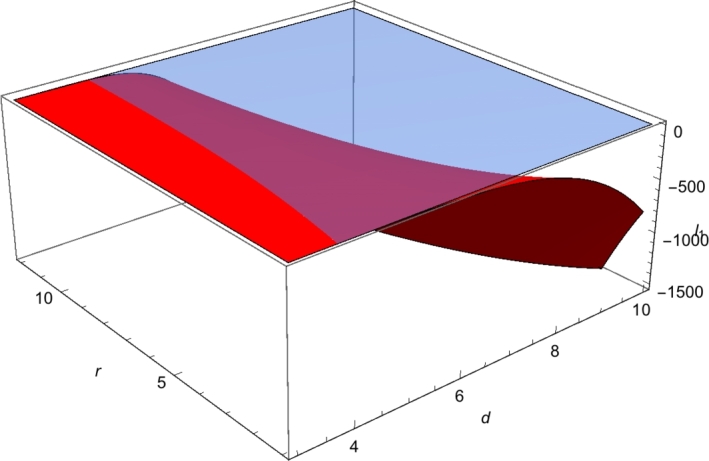
First Lyapunov coefficient ℓ₁(a₀;d,r) with K = 4 and m = 2. The plane z = 0 is in blue color and the positive graph of ℓ₁ is in red color.

Lemma 3.2

If $d>1$ , $d\ne 4$ , $r>\frac{16-2d^3+6d^2-8d}{d}$ and $\mu (a;d,r)$ is the real part of the complex eigenvalues of $J(P_0(c_0,{\alpha }_0))$ , then

$$\frac{\partial \mu (a;d,r)}{\partial a}{|}_{a=a_0}\ne 0.$$

Proof

By Lemma 3.1, we have that differential system (1), has purely imaginary eigenvalues, when the parameter a satisfies the condition (9). Then, we just need to verify the following transversality condition to have a Hopf bifurcation at $P_0(c_0,{\alpha }_0)$ with respect to parameter a. That is, we need to show that the derivative of $\mu (a;d,r)$, the real part of the eigenvalues of the linear approximation at $P_0(c_0,{\alpha }_0)$, with respect to a is different to zero. We have

$$\frac{\partial \mu (a;d,r)}{\partial a}{|}_{a=a_0}=\frac{(d-4)(d-1)(4-d+d^2){(2d^3-6d^2+d(8+r)-16)}^2}{384d^{3}r}.$$

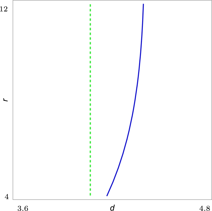
Since $2d^3-6d^2+d(8+r)-16>0$ when $r>\frac{16-8d+6d^2-2d^3}{d}$, we have $\frac{\partial \mu (a;d,r)}{\partial a}{|}_{a=a_0}$ is nonzero, if the hypotheses of the lemma are satisfied, see Fig. 2.

Figure 2.

The continuous line is the zero level curve of ℓ₁(d,r). The dashed line is the curve $\frac{\partial \mu (a;d,r)}{\partial a}{|}_{a=a_0}=0$.

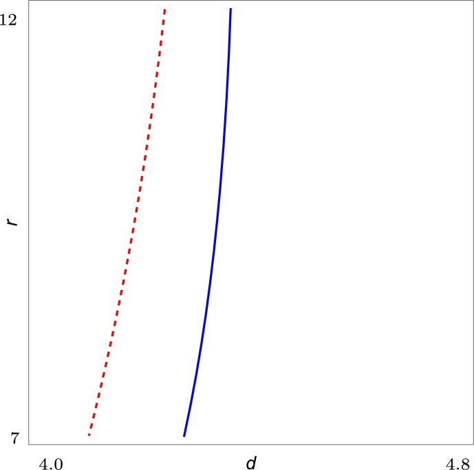
In order to prove that the differential system (1) exhibits a Bautin bifurcation at $P_0(c_0,{\alpha }_0)$, we need to calculate the second Lyapunov coefficient ${\ell }_2(d,r)$ for the parameters where ${\ell }_1=0$. This coefficient is calculated using a Kuznetsov's formula (see [9]) and Mathematica (see Appendix A.7). From Appendix A.7, we have that ${\ell }_2(d,r)\ne 0$ on the zero level set of ${\ell }_1(d,r)$, see Fig. 3.

Figure 3.

The continuous line is the zero level curves of ℓ₁(d,r). The dashed line is the curve where ℓ₂(d,r)=0.

We set the parameters values used to calculate ${\ell }_1(d,r)$ and we define

$$\mathcal{R}=\{(d,r)\in {\mathbb{R}}^2:a_0>0,c_0>0\text{ and }{\alpha }_0>0)\},$$

Lemma 3.3

Let

$$\mathrm{\Gamma }=\{(d,r)\in \mathcal{R}:{\ell }_1(d,r)=0\mathit{\text{and}}{\ell }_2(d,r)\ne 0\},$$

and let$\mu (a;d,r)$be the real part of the eigenvalues of$J(P_0(c_0,{\alpha }_0))$. Then the map${\varphi }_1(d,r)={(\mu (a;d,r),{\ell }_1(a;d,r))}^T$is regular on Γ.

Proof

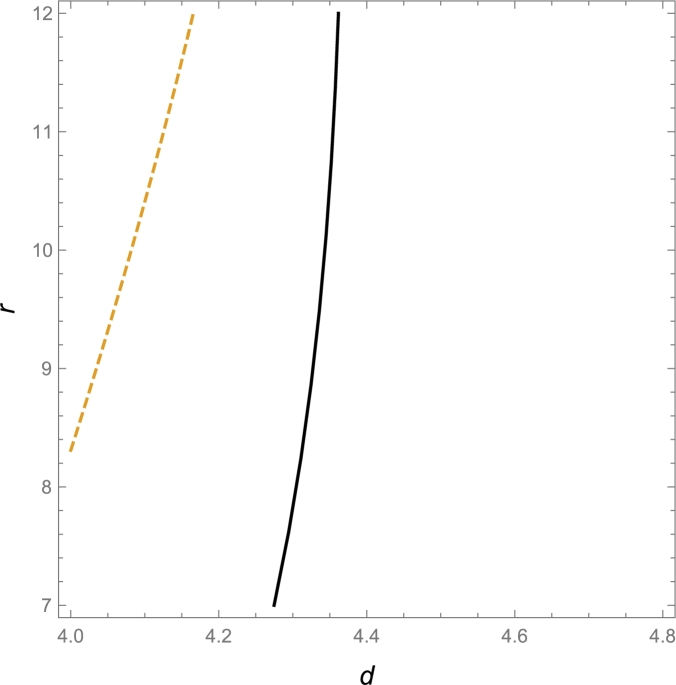
In the expression (11) we show the first Lyapunov coefficient, when $J(P_0(c_0,{\alpha }_0))$ has purely imaginary eigenvalues. In order to show the regularity of map ${\varphi }_1$, we need to calculate the first Lyapunov coefficient in a neighborhood of $a_0$. Since the expression of determinant of the Jacobian matrix of the map ${\varphi }_1$ is too large, in Fig. 4 we show where it is zero in the region of parameters $d-r$. In particular, this determinant is different from zero, when ${\ell }_1$ is zero. Therefore, the function ${\varphi }_1$ is regular on the set Γ.

Figure 4.

The continuous line is the zero level curve of ℓ₁(d,r). The dashed line is the zero level curve of Jacobian matrix determinant of map ϕ₁(d,r).

In summary we have,

Theorem 3.1

[Main Theorem]. If $(d,r)\in \mathrm{\Gamma }$ then system (1) exhibits a Bautin's bifurcation at equilibrium point $P_0(c_0,{\alpha }_0)$ .

4. Numerical simulations

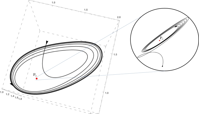
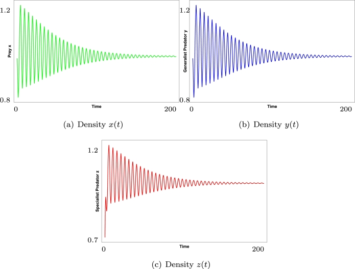
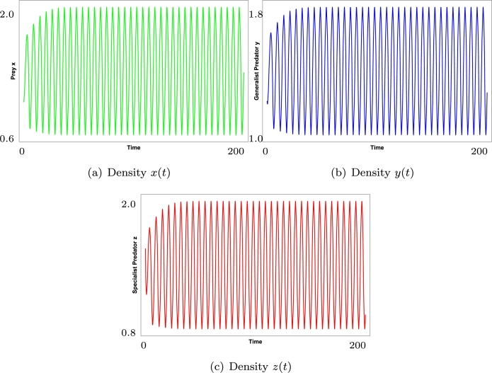
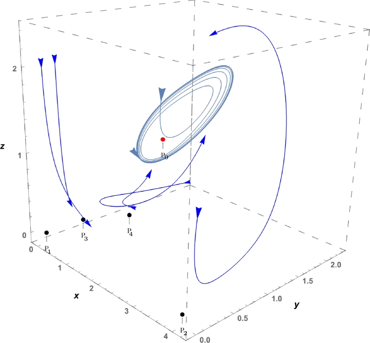
We choose the values of the parameters in system (1) in such a way that the hypothesis of Theorem 3.1 is satisfied. We fix $m=2$, $n=1$, $b=1$, $q=\frac{25}{2}$, $\mu =\frac{20}{3}$, $q_1=1$, $d=4$, $r=8$, $a_0=1.5$, $c_0=\frac{1}{2}$, ${\alpha }_0=\frac{5}{2}$ and $K=4$. Then system (1) exhibits a Bautin bifurcation. In this case $P_0=(1,1.2,1)$ is a stable equilibrium point and there are two limit cycles around it, see Fig. 5. In Fig. 6 we show the time series for the densities of prey, generalist predator and specialist, entering through the stable manifold. Starting in $x_0=(1,1.2,1.5)$ the population densities oscillate in $x\in (0.68,2)$, $y\in (1,1.8)$ and $z\in (0.8,2)$, see Fig. 7. In addition of $P_0$, system (1) has four equilibrium points in the closure of the positive octant $P_1=(0,0,0)$, $P_2=(4,0,0)$, $P_3=(0,0.5,0)$ and $P_4=(0.47,0.97,0)$, which are saddle points. The eigenvalues of $J(P_1)$ are ${\lambda }_1=8$, ${\lambda }_2=-4$ and ${\lambda }_3=2.5$. $J(P_2)$ has eigenvalues ${\lambda }_1=-8$, ${\lambda }_2=-4$ and ${\lambda }_3=2.5$. The eigenvalues of $J(P_3)$ are ${\lambda }_1=3.8$, ${\lambda }_2=-2.5$ and ${\lambda }_3=-0.6$. Finally for $J(P_4)$, the eigenvalues are ${\lambda }_1=-0.80+2.39i$, ${\lambda }_2=-0.80-2.39i$ and ${\lambda }_3=2.51$, see Fig. 8.

Figure 5.

Starting from the initial condition x₀ = (1,1.2,1.5) the orbit tends to a stable limit cycle. With x₀ = (0.99,1.2,0.7) the orbit tends to the equilibrium point P₀ = (1,1.2,1). Since the equilibrium point and the periodic orbit are stables, there is an unstable limit cycle in the central manifold.

Figure 6.

Time series with x₀ = (0.99,1.2,0.7) entering the stable manifold, a = 1.5 and K = 4.

Figure 7.

Time series with x₀ = (1,1.2,1.5) for the stable periodic orbit, a = 1.5 and K = 4.

Figure 8.

Local dynamics of system (1) around of equilibrium points in the positive octant.

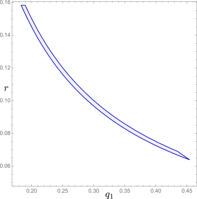
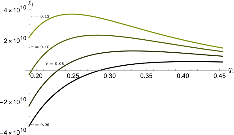
Setting the parameters $m=2$, $q=0.78$, $\mu =0.21$, $a=0.98$, $c=0.02$, $\alpha =0.39$, $d=0.01$, $K=30$, $b=0.0002$, $n=1$ and leaving the parameters free r, $q_1$, system (1) satisfies the conditions (4) and (9). In Fig. 9 we show the feasible region of parameters and the Fig. 10 shows the behavior of the first Lyapunov coefficient as function of r and $q_1$.

Figure 9.

Feasible region where the parameters of system (1) are positive and the conditions for the Hopf bifurcation are satisfied.

Figure 10.

Behavior of ℓ₁ varying r and q₁.

5. Conclusion

In this work, we analyze the dynamics of a intraguild model where the numerical response of the mesopredator is of the Leslie-Gower type and the prey has a density-dependent defense mechanism. The top predator is a specialist and feeds only on the mesopredator, which is a generalist. We show conditions in the system parameters that guarantee the coexistence of the three populations, which can occur through an equilibrium point or a stable limit cycle. Furthermore, we show that bi-stability can occur because there are conditions to have two stable limit sets simultaneously, one of which is an equilibrium point and the other a limit cycle. In order to show the existence of a stable limit cycle, we have determined conditions for a Hopf bifurcation. In particular, when m = 2 it is shown the existence of supercritical and subcritical Hopf bifurcations. The system also presents Bautin Bifurcation, see Fig. 5. Although, the first Lyapunov coefficient has been calculated for system (1) as a function of the growth rate of the prey and the mortality rate of the specialist predator, it is worth mentioning that it can also be calculated as a function of parameters such as the defense mechanism of the prey, the growth rate of the prey, and the mortality rate of the specialist predator, among others.

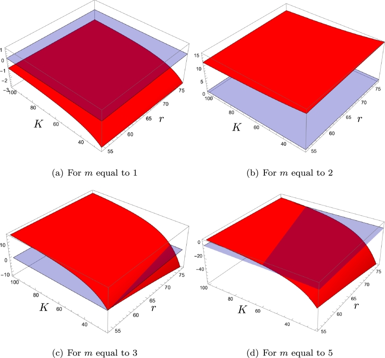
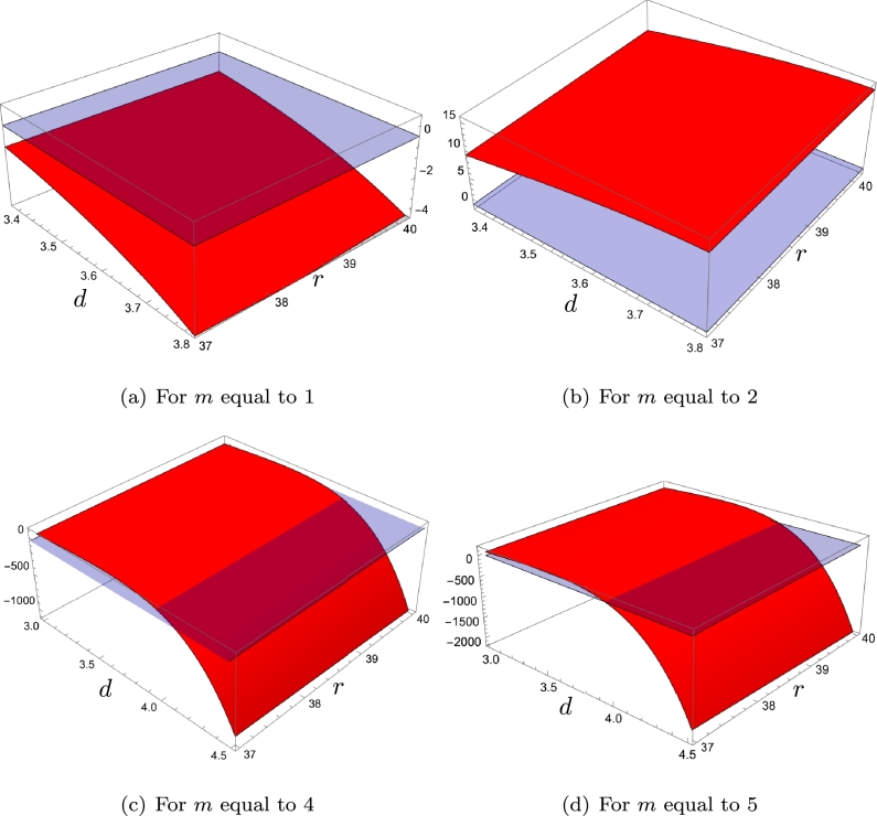
In order to get some insight about the role of the prey defense mechanism on the stability of the system we performed some numerical simulations to explore different scenarios. In Figure 11, Figure 12 we show in red the graph of ${\ell }_1$ compared to the plane $z=0$ (in blue), in order to identify when a supercritical or subcritical Hopf bifurcation occurs. In Fig. 11, the superpredator mortality rate is fixed $d=4$ and $K,r$ are free parameters; in absence of defense ($m=1$), population fluctuations derived from a Hopf bifurcation are stable, favoring the extinction of some of the species because an environmental perturbation when the population size of some of the species is low enough could drive that species to unrecoverable level (See [10], and [5]). A medium defensive level ($m=2$) allows to damp the fluctuations and the populations tend to a stable equilibrium level. However, as the prey defensive level increases, greater carrying capacities are needed to achieve coexistence of the three species through a stable equilibrium point $(m=3,5)$. In Fig. 12, we consider the carrying capacity $K=10$ and $r,d$ are free parameters; as in the previous scenario, if $m=1$, the system presents stable limit cycles and for $m=2$ these cycles appear but are unstable, however coexistence occurs through a stable equilibrium point. In the case of high levels of defense ($m=4,5$), damping population fluctuations requires that d be large enough.

Figure 11.

First Lyapunov coefficient (in red color) as a function of K and r, for m = 1,2,3,5 and d = 4. The plane z = 0 is in blue color.

Figure 12.

First Lyapunov coefficient (in red color) as a function of d and r, for m = 1,2,4,5 and K = 10. The plane z = 0 is in blue color.

The proof of a Bautin bifurcation for system (1) guarantees that for certain parameters there exist attractive sets consisting of a stable equilibrium point and a stable periodic orbit. So, the $\omega -\text{Limit}$ of a orbit depends on the initial population of prey and predators. This can be interpreted from an ecological point of view, as the emergence of two niches as a consequence of the interaction mechanisms, the intensity of which depends on the parameters involved. The relation between the selection pressures of competition among species and the niche width has been experimentally studied in [12].

Ethical approval

This article does not contain any studies with human participants or animals performed by any of the authors.

Funding statement

The research did not receive any funding.

CRediT authorship contribution statement

Gamaliel Blé: Writing – review & editing, Writing – original draft, Methodology, Investigation, Formal analysis, Conceptualization. Luis Miguel Valenzuela: Writing – review & editing, Writing – original draft, Methodology, Investigation, Formal analysis, Conceptualization. Manuel Falconi: Writing – review & editing, Writing – original draft, Validation, Methodology, Investigation, Formal analysis, Conceptualization.

Declaration of Competing Interest

The authors declare that they have no known competing financial interests or personal relationships that could have appeared to influence the work reported in this paper.

Appendix A.

A.1. Kuznetsov's formula for the first Lyapunov coefficient

$${\ell }_1=\frac{1}{2\omega }Re(\overline{p}\cdot C(q,q,\overline{q})-2\overline{p}\cdot B(q,A^{-1}B(q,\overline{q}))+\overline{p}\cdot B(\overline{q},{(2\omega iI-A)}^{-1}B(q,q))),$$ (A.1)

where I denotes the identity matrix.

A.2. Linear forms

$$A=\left(\begin{array}{ccc}\hfill A_{1,1}\hfill & \hfill A_{1,2}\hfill & \hfill 0\hfill \\ \hfill \hfill \\ \hfill A_{2,1}\hfill & \hfill A_{2,2}\hfill & \hfill A_{2,3}\hfill \\ \hfill \hfill \\ \hfill 0\hfill & \hfill A_{3,2}\hfill & \hfill -\frac{d}{2}\hfill \end{array}\right)$$

where

$$A_{1,1}=\frac{(4-\frac{8}{d}-3d+d^2)}{2},A_{1,2}=-((4+(-1+d)d)(-8+d(7+(-4+d)d))(16+d(-16+d(13+(d-6)d))/(2d{(-8+d(6+(-4+d)d))}^2),A_{2,1}=\frac{{(-8+d(6+(-4+d)d))}^2}{2d(-8+d(7+(-4+d)d))},A_{2,2}=-3+\frac{4}{d}+2d-\frac{d^2}{2},A_{2,3}=d{(-8+d(6+(d-4)d))}^2(K-1)r/(2(4+(-1+d)d))(-8+d(7+(d-4)d))(16+d(-16+d(13+(d-4)d)))K,A_{3,2}=4+(d-1)d)(-8+d(7+(-4+d)d))(16+d(-16+d(13+(d-6)d)))K/(2{(-8+d(6+(d-4)d))}^2(-1+K)r).$$

A.3. Bilinear and trilinear forms

$$B(x,y,z,u,v,w)=(B_1((x,y,z),(u,v,w)),B_2((x,y,z),(u,v,w)),B_3((x,y,z),(u,v,w))),$$

where

$$\begin{gathered} B_1((x,y,z),(u,v,w))=-((2{(-8+d(6+(-4+d)d))}^2(-8+d(4+(-3+d)d))K^2(-8+d(4+(d-3)d-3r))ux+12d^2{(-8+d(6+(d-4)d))}^2{r}^{2}ux+2d((-8+d(6+(d{-4)d))}^2)Kr(-56+7d(4+(d-3)d)-2dr)ux-(4+(d-1)d)(-8+d(7+(d-4)d))(16+d(-16+d(13+(d-6)d)))K^2(-8+d(4+(d-3)d-2r))vx-4d(4+(-1+d)d)(-8+d(7+(-4+d)d))(16+d(-16+d(13+(-6+d)d)))Krvx-(4+(d-1)d)(-8+d(7+(d-4)d))(16+d(-16+d(13+(d-6)d)))K(K(-8+d(4+(d-3)d-2r))+4dr)uy)/(4d^2{(-8+d(6+(-4+d)d))}^2(K-1)Kr)),B_2((x,y,z),(u,v,w))=\frac{1}{4}((2(4+(-1+d)d)(16+d(-16+d(13+(-6+d)d)))Kvx)/(d^2(-1+K)r)-(2(4+(-1+d)d)(16+d(-16+d(13+(-6+d)d)))Kvy)(16+d(-16+d(13+(-6+d)d)))Kvy)/(d^2(-8+d(6+(-4+d)d))(-1+K)r)+((wy)/(-1+K))-(Kwy)/(-1+K)-(2(4+(-1+d)d)(16+d(-16+d(13+(-6+d)d)))Ku(-8x+d(6+(-4+d)d)x+8y-d(7+(-4+d)d)y))/(d^2(-8+d(7+(-4+d)d))(-1+K)r)-vz+(2d({(-8+d(6+(-4+d)d))}^2)(-1+K)r \\ wz)/((4+(-1+d)d)(-8+d(7+(-4+d)d))(16+d(-16+d(13+(-6+d)d)))K))B_3((x,y,z),(u,v,w))=((4+(-1+d)d)(-8+d(7+(-4+d)d))(16+d(-16+d(13+(-6+d)d)))Kwy+((4+(-1+d)d)(-8+d(7+(-4+d)d))(16+d(-16+d(13+(-6+d)d)))Kv-2d{(-8+d(6+(-4+d)d))}^2(-1+K)rw)z)/(4(-8+d{(6+(-4+d)d))}^2(-1+K)r). \end{gathered}$$

And the trilinear form C at $(0,0)$ is

$$\begin{gathered} C((x,y,z),(u,v,w),(r_1,s,t))=(C_1,C_2,C_3),\text{ and } \\ {C}_1=C_1((x,y,z),(u,v,w),(r_1,s,t))C_2=C_2((x,y,z),(u,v,w),(r_1,s,t))C_3=C_3((x,y,z),(u,v,w),(r_1,s,t)) \end{gathered}$$

where

$$C_1=(1/(4d^3{(-1+K)}^2{r}^2))((-8+d(4+(-3+d)d))K+2dr)(3r_1({(-8+d(4+(-3+d)d))}^2{K}^2-4d(-8+d(4+(-3+d)d))(-2+K)Kr+2d^2(7+(-6+K)K)r^2)ux)/K-(1/({(-8+d(6+(-4+d)d))}^2))(4+(-1+d)d)(-8+d(7+(-4+d)d))(16+d(-16+d(13+(-6+d)d)))(K(-8+d(4+(-3+d)d-3r))+5dr)(sux+r_{1}vx+r_{1}uy))C_2=1/4(({(4+(-1+d)d)}^2(-8+d(7+(-4+d)d))(16+d(-16+d(13{+(-6+d)d)))}^2{K}^{2}svx)/(d^3{(-8+d(6+(-4+d)d))}^2{(-1+K)}^2{r}^2)+((twy)/{(-1+K)}^2)-(2Ktwy)/{(-1+K)}^2+(K^{2}twy)/{(-1+K)}^2-({(4+(-1+d)d)}^2(16+d(-16+d(13+(16+d(-16+d(13{+(-6+d)d)))}^2{K}^{2}su(2(-8+d(6+(-4+d)d))x+8y-d(7+(-4+d)d)y))/d^3{(-8+d(6+(-4+d)d))}^2{(-1+K)}^2{r}^2+({(4+(-1+d)d)}^2{(16+d(-16+d(13+(-6+d)d)))}^2)(K^2)r_1((-8+d(6+(-4+d)d))u(3(-8+d(6+(-4+d)d))x-2(-8+d(7+(-4+d)d))y)+(-8+d(7+(-4+d)d))v(-2(-8+d(6+(-4+d)d))x+(-8+d(7+(-4+d)d))y)))/(d^3{(-8+d(6+(-4+d)d))}^2(-8+d(7+(-4+d)d)){(-1+K)}^2{r}^2)+(sw+t(v-(3d{(-8+d(6+(-4+d)d))}^2(-1+K)rw)/(4+(-1+d)d)(-8+d(7+(-4+d)d))(16+d(-16+d(13+(-6+d)d)))K))z)C_3=(3/4)dtwz-(4+(-1+d)d)(-8+d(7+(-4+d)d))(16+d(-16+d(13+(-6+d)d)))K(twy+tvz+swz)/4(-8{+d(6+(-4+d)d))}^2(-1+K)r.$$

A.4. h value

$$\begin{gathered} h=1/((((32768-102400d+194816d^2-261504d^3+271840d^4-227112d^5+155813d^6-88768d^7+42040d^8-16472d^9+5258d^{10}-1328d^{11}+252d^{12}-32d^{13}+2d^{1}4)r^2-2(32768-102400d+194816d^2-261504d^3+271840d^4-227112d^5+155813d^6-88768d^7+42040d^8-16472d^9+5258d^{10}-1328d^{11}+252d^{12}-32d^{13}+2d^{14})K{r}^2+K^2(-1680d^{15}+237d^{16}-22d^{17}+d^{18}+32768(8+r^2)+2d^{14}(4417+r^2)-4d^{13}(9165+8r^2)-4096d(272+25r^2)+2d^{12}(62233+126r^2)-8d^{11}(44197+166r^2)+256d^2(10576+761r^2)-128d^3(36464+2043r^2)+d^{10}(852301+5258r^2)-2d^9(878899+8236r^2)+32d^4(195192+8495r^2)-8d^7(592083+11096r^2)-8d^5(849088+28389r^2)+d^8(3113761+42040r^2)+d^6(6161648+155813r^2)))/((-512+1088d-1488d^2 \\ {{+1396d^3-971d^4+513d^5-202d^6+58d^7-11d^8+d^9)}^2{K}^2))}^{\frac{1}{2}}) \end{gathered}$$

A.5. $h_1$ value

$$\begin{gathered} h_1=1/(1/((((32768-102400d+194816d^2-261504d^3+271840d^4-227112d^5+155813d^6-88768d^7+42040d^8-16472d^9+5258d^{10}-1328d^{11}+252d^{12}-32d^{13}+2d^{14})r^2-2(32768-102400d+194816d^2-261504d^3+271840d^4-227112d^5+155813d^6-88768d^7+42040d^8-16472d^9+5258d^{10}-1328d^{11}+252d^{12}-32d^{13}+2d^{14})K{r}^2+K^2(-1680d^{15}+237d^{16}-22d^{17}+d^{18}+32768(8+r^2)+2d^{14}(4417+r^2)-4d^{13}(9165+8r^2)-4096d(272+25r^2)+2d^{12}(62233+126r^2)-8d^{11}(44197+166r^2)+256d^2(10576+761r^2)-128d^3(36464+2043r^2)+d^{10}(852301+5258r^2)-2d^9(878899+8236r^2)+32d^4(195192+8495r^2)-8d^7(592083+11096r^2)-8d^5(849088+28389r^2)+d^8(3113761+42040r^2)+d^6(6161648+155813r^2)))/((-512+1088d-1488d^2 \\ {{+1396d^3-971d^4+513d^5-202d^6+58d^7-11d^8+d^9)}^2{K}^2))}^{\frac{1}{2}})+((-4i+((-3+2i)+d)d)(4+(-1+d)d))/(d(4i+((-3-2i)+d)d)(((32768-102400d+194816d^2-261504d^3+271840d^4-227112d^5+155813d^6-88768d^7+42040d^8-16472d^9+5258d^{10}-1328d^{11}+252d^{12}-32d^{13}+2d^{14})r^2-2(32768-102400d+194816d^2-261504d^3+271840d^4-227112d^5+155813d^6-88768d^7+42040d^8-16472d^9+5258d^{10}-1328d^{11}+252d^{12}-32d^{13}+2d^{14})K{r}^2+K^2(-1680d^{15}+237d^{16}-22d^{17}+d^{18}+32768(8+r^2)+2d^{14}(4417+r^2)-4d^{13}(9165+8r^2)-4096d(272+25r^2)+2d^{12}(62233+126r^2)-8d^{11}(44197+166r^2)+256d^2(10576+761r^2)-128d^3(36464+2043r^2)+d^{10}(852301+5258r^2)-2d^9(878899+8236r^2)+32d^4(195192+8495r^2)-8d^7(592083+11096r^2)-8d^5(849088+28389r^2)+d^8(3113761+42040r^2)+d^6(6161648+155813r^2)))/((-512+1088d-1488d^2+1396d^3-971d^4+513d^5 \\ {{-202d^6+58d^7-11d^8+d^9)}^2{K}^2))}^{\frac{1}{2}})-({(2i+d)}^2(4i+((-3-2i)+d)d)(-4i+((-3+2i)+d)d))/(d(16+d(-16+d(13+(-6+d)d)))(((32768-102400d+194816d^2-261504d^3+271840d^4-227112d^5+155813d^6-88768d^7+42040d^8-16472d^{9}5258d^{10}-1328d^{11}+252d^{12}-32d^{13}+2d^{14})r^2-2(32768-102400d+194816d^2-261504d^3+271840d^4-227112d^5+155813d^6-88768d^7+42040d^8-16472d^9+5258d^{10}-1328d^{11}+252d^{12}-32d^{13}+2d^{14})K{r}^2+K^2(-1680d^{15}+237d^{16}-22d^{17}+d^{18}+32768(8+r^2)+2d^{14}(4417+r^2)-4d^{13}(9165+8r^2)-4096d(272+25r^2)+2d^{12}(62233+126r^2)-8d^{11}(44197+166r^2)+256d^2(10576+761r^2)-128d^3(36464+2043r^2)+d^{10}(852301+5258r^2)-2d^9(878899+8236r^2)+32d^4(195192+8495r^2)-8d^7(592083+11096r^2)-8d^5(849088+28389r^2)+d^8(3113761+42040r^2)+d^6(6161648+155813r^2)))/((-512+1088d-1488d^2+1396d^3 \\ {{-971d^4+513d^5-202d^6+58d^7-11d^8+d^9)}^2{K}^2))}^{\frac{1}{2}})). \end{gathered}$$

A.6. First Lyapunov coefficient for $K=4$

$$S_1=(-268435456+1241513984d-2751463424d^2+4011851776d^3-4100980736d^4+2827485184d^5-878510080d^6-781852672d^7+1583149056d^8-1568899584d^9+1130110464d^{10}-644749312d^{11}+300256064d^{12}-115241792d^{13}+36416832d^{14}-9390848d^{15}+1941952d^{16}-313280d^{17}+37696d^{18}-3072d^{19}+128d^{20}-33554432r-62914560dr+562036736d^{2}r-1575223296d^{3}r+2868641792d^{4}r-3933454336d^{5}r+4340580352d^{6}r-3992841216d^{7}r+3125515776d^{8}r-2108147584d^{9}r+1233252224d^{10}r-627087936d^{11}r+276672992d^{12}r-105301824d^{13}r+34222736d^{14}r-9346464d^{15}r+2093424d^{16}r-370432d^{17}r+48624d^{18}r-4192d^{19}r+176d^{20}r+8388608r^2-60817408d{r}^2+204210176d^2{r}^2-455081984d^3{r}^2+746110976d^4{r}^2-967663616d^5{r}^2+1029989376d^6{r}^2-922621952d^7{r}^2+706464960d^8{r}^2-466923648d^9{r}^2+267912592d^{10}{r}^2-133745744d^{11}{r}^2+58042928d^{12}{r}^2-21807320d^{13}{r}^2+7033252d^{14}{r}^2-1919216d^{15}{r}^2+432684d^{16}{r}^2-77432d^{17}{r}^2+10252d^{18}{r}^2-880d^{19}{r}^2+36d^{20}{r}^2-1048576d{r}^3+7077888d^2{r}^3-20889600d^3{r}^3+40050688d^4{r}^3-56535040d^5{r}^3+62779392d^6{r}^3-56898752d^7{r}^3+43048992d^8{r}^3-27550224d^9{r}^3+15008304d^{10}{r}^3-6961152d^{11}{r}^3+2733176d^{12}{r}^3-896516d^{13}{r}^3+240068d^{14}{r}^3-50504d^{15}{r}^3+7792d^{16}{r}^3-772d^{17}{r}^3+36d^{18}{r}^3+32768d^2{r}^4-196608d^3{r}^4+510976d^4{r}^4-862208d^5{r}^4+1064192d^6{r}^4-1016832d^7{r}^4+775964d^8{r}^4-479592d^9{r}^4+241140d^{10}{r}^4-98112d^{11}{r}^4+31763d^{12}{r}^4-7930d^{13}{r}^4+1436d^{14}{r}^4-166d^{15}{r}^4+9d^{16}{r}^4),$$

$$S_2=(4194304-17825792d+43319296d^2-74678272d^3+99938304d^4-108683264d^5+98586368d^6-75786624d^7+49820176d^8-28124768d^9+13636816d^{10}-5657216d^{11}+1991456d^{12}-586560d^{13}+141344d^{14}-26880d^{15}+3792d^{16}-352d^{17}+16d^{18}+294912r^2-921600d{r}^2+1753344d^2{r}^2-2353536d^3{r}^2+2446560d^4{r}^2-2044008d^5{r}^2+1402317d^6{r}^2-798912d^7{r}^2+378360d^8{r}^2-148248d^9{r}^2+47322d^{10}{r}^2-11952d^{11}{r}^2+2268d^{12}{r}^2-288d^{13}{r}^2+18d^{14}{r}^2).$$

A.7. Second Lyapunov coefficient

$${\ell }_2(d,r)=((16-16d+13d^2-6d^3+d^4)(-32+36d-31d^2+15d^3{-5d^4+d^5)}^4(-844424930131968r^2(192-24r+7r^2)+48d^{44}{r}^2(192+24r+7r^2)-96d^{43}r(-3072+4800r+512r^2+181r^3)+48d^{42}r(-329216+234336r+20712r^2+9217r^3+14r^4)+70368744177664d(-77824-20480r+15936r^2-2880r^3+792r^4+21r^5)-96d^{41}(-53248-4355840r+1858352r^2+129232r^3+77188r^4+341r^5)-2199023255552d^2(-19398656-3772416r+1587200r^2-423936r^3+118968r^4+6252r^5+63r^6)+8d^{40}(-30193664-910379264r+258235584r^2+12623088r^3+11503194r^4+97740r^5+63r^6)-32d^{39}(-174891008-2933901696r+581891808r^2+14215152r^3+28286217r^4+383028r^5+720r^6)+274877906944d^3(-671023104-91938816r+16342016r^2-9111168r^3+3052416r^4+233496r^5+4446r^6+21r^7)+8d^{38}(-10591157248-119386575360r+17008454336r^2-114459984r^3+918706902r^4+17791860r^5+64404r^6+21r^7)-8d^{37}(-117821836288-998034355712r+103664529216r^2-5062614912r^3+6332876424r^4+163691772r^5+943410r^6+897r^7)-4294967296d^4(-132356505600-11231690752r-2015772672r^2-925317120r^3+487259904r^4+47108352r^5+1268928r^6+11088r^7+21r^8)+d^{36}(-8215471067136-56399303616512r+4305685504512r^2-465564422016r^3+302399080176r^4+9959458464r^5+81770040r^6+149640r^7+21r^8)+2147483648d^5(-642372861952-22670868480r-29935607808r^2-668497920r^3+2034597888r^4+225183936r^5+7650144r^6+93588r^7+321r^8)-2d^{35}(-29210051182592-171787323645952r+9681976412672r^2-1876248479232r^3+792765887760r^4+32223757824r^5+350429640r^6+1019868r^7+417r^8)268435456d^6(-10346548953088+141833404416r-755808600064r^2+47933079552r^3+29783280384r^4+3477134976r^5+139691712r^6+2148144r^7+10233r^8)-16d^{33}(-111173323777024-542215077887488r+16893089445472r^2-8461064510688r^3+1921069511520r^4+112187530002r^5+1862891976r^6+10176255r^7+12723r^8)+536870912d^7(-8918961750016+570226851840r-856725612544r^2+91194406656r^3+24557810304r^4+2816025744r^5+128167140r^6+2340942r^7+13977r^8)+d^{34}(-348467049246720-1833362354466816r+76560461819392r^2-24421059912576r^3+7380358062864r^4+362207821344r^5+4958570208r^6+20516640r^7+16137r^8)-16777216d^8(-430169094356992+50422353756160r-50110850973696r^2+6834995165184r^3+1185127372032r^4+125551290624r^5+6267093888r^6+131374512r^7+931773r^8)+2d^{32}(-3942907869573120-18383078754102272r+434598381410560r^2-328630270640832r^3+57580001690424r^4+3966928007184r^5+77690416404r^6+531657000r^7+944349r^8)8388608d^9(-1149993073770496+202022376636416r-155218105147392r^2+25044859103232r^3+3286389920256r^4+305689500864r^5+16289474496r^6+383377716r^7+3129105r^8)-4d^{31}(-7673098889027584-35169773946870784r+654930612972800r^2-710703344578176r^3+97361339764920r^4+7887776788896r^5+178280112024r^6+1469830956r^7+3442191r^8)+2097152d^{11}(-5956887849467904+1903281819615232r-1001309913606144r^2+208160468553984r^3+19622586001152r^4+1240710151920r^5+70078249044r^6+2015555538r^7+20755119r^8)-1048576d^{10}(-11018591697633280+2665972365787136r-1675018375561216r^2+309211351572480r^3+33523264867584r^4+2623162222464r^5+145638984384r^6+3797630928r^7+34989417r^8)+2d^{30}(-52830214565814272-244625153213798400r+3845438115165440r^2-5540667674770368r^3+595068068185992r^4+56826636193584r^5+1457029304208r^6+14041411188r^7+41094273r^8)-8d^{2}9(-40385076347571200-194385163349429760r+2859826592869824r^2-4906740636143616r^3+410202505919592r^4+46595056618932r^5+1336649421570r^6+14697932829r^7+51614721r^8)-65536d^{12}(-187097765727174656+77272788235845632r-34362057750822912r^2+7984371986847744r^3+673723543602432r^4+32814462484224r^5+1835576696640r^6+58748491440r^7+675961911r^8)+32768d^{13}(-334712304502833152+177038344919580672r-66675488487956480r^2+17264702144182272r^3+1323281494742016r^4+46037972965440r^5+2451652338528r^6+90756596220r^7+1183891635r^8)+d^{28}(-877760326427365376-4538254447662299136r+70320914832210432r^2-127154377716898560r^3+8120332477170048r^4+1117486309972320r^5+35464348058088r^6+436225995240r^7+1779607041r^8)+8192d^{15}(-817713257119481856+711284310164979712r-190287852653336576r^2+61257611596971264r^3+3899511440180352r^4+28485291835440r^5+301192485948r^6+103149389922r^7+2215423977r^8)+64d^{24}(-155389879470813696-2340752971952845568r+87647737165433760r^2-96982740191846640r^3+775293035170164r^4+597836255497350r^5+26310148131981r^6+436379879289r^7+2545810371r^8)-2d^{27}(-1053886982970425344-6103254712195706880r+110215115794459136r^2-189228611437458432r^3+8907353560300032r^4+1535299373577984r^5+53407977722472r^6+722647252524r^7+3333853185r^8)-4096d^{14}(-2188215091018596352+1480485903630467072r-471121501787324416r^2+135910216204812288r^3+9506760070891776r^4+201362217592704r^5+9246396331968r^6+457434487632r^7+7089743139r^8)+3d^{26}(-1468234653002993664-10118226186312683520r+227357417768505344r^2-346283263498809856r^3+11248031941365760r^4+2582386231087808r^5+97724295809312r^6+1433469503984r^7+7305363663r^8)8d^{25}(-962224457384247296-8746160484494945280r+252469768544931840r^2-329684207347847808r^3+6454276157604768r^4+2245234044540720r^5+91857138030636r^6+1441649070948r^7+7943655543r^8)-128d^{21}(990758596668948480-7482506397190718976r+591303317791840256r^2-406360341492367776r^3-8559499698059904r^4+1699461462844752r^5+91354647527535r^6+1652170893909r^7+9791136957r^8)+128d^{17}(-22254568232745697280+33278583289382109184r-6156948434947407872r^2+2493467442779215872r^3+127075010745650688r^4-3161895927031872r^5-239878599639936r^6-2609811602628r^7+19654371387r^8)-16d^{23}(-238588268048252928-18650669096061393920r+903730715766499328r^2-847598348435030784r^3-2140361103758880r^4+4673629163273040r^5+220384875273252r^6+3815675402580r^7+23050293543r^8)-256d^{16}(-17874411634629279744+20208491043648176128r-4514121777692508160r^2+1626528155928637440r^3+93368592526803456r^4-714855464060160r^5-80296900849920r^6+346387185360r^7+34528249575r^8)+16d^{18}(100353825195118559232-203805759567900311552r+30950250313026732032r^2-14161589492433543168r^3-625875698170705920r^4+28946813198494464r^5+1933919930124576r^6+29703564310608r^7+49378784133r^8)-32d^{19}(25280860468040040448-72650201019956281344r+8967975813348200448r^2-4664815030518564864r^3-172619505072950016r^4+12979550146691040r^5+798306822534960r^6+13737869489772r^7+58984580289r^8)+8d^{22}(3644345857682251776-69211740905320046592r+4305072880789016576r^2-3442544969728799232r^3-41883293283189024r^4+16711931681232672r^5+842018413399104r^6+15017770552224r^7+91499272551r^8)+16d^{20}(22169421244207464448-96569780537895223296r+9589677588916692992r^2-5711044461102391296r^3-167431597828137216r^4+19948645593441600r^5+1144634337760104r^6+20545684994952r^7+111368286567r^8)))/(150994944d^8{(-8+6d-4d^2+d^3)}^4(-26880d^{15}+3792d^{16}-352d^{17}+16d^{18}-96d^{13}(6110+3r^2)+32768(128+9r^2)+2d^{14}(70672+9r^2)-4096d(4352+225r^2)+4d^{12}(497864+567r^2)-16d^{11}(353576+747r^2)-576d^7(131574+1387r^2)+256d^2(169216+6849r^2)+288d^4(347008+8495r^2)-128d^3(583424+18387r^2)-8d^9(3515596+18531r^2)+2d^{10}(6818408+23661r^2)+8d^8(6227522+47295r^2)-8d^5(13585408+255501r^2){+d^6(98586368+1402317r^2))}^2).$$

Data availability statement

No data was used for the research described in the article.

References

- 1.Blé G., Dela Rosa M.A. Bogdanov-Takens bifurcation in a Leslie type tritrophic model with general functional responses. Acta Appl. Math. 2020;169:361–382. doi: 10.1007/s10440-019-00302-z. [DOI] [Google Scholar]
- 2.Blé G., Loreto I. Limit cycles in a tritrophic food chain model with general functional responses. Int. J. Nonlinear Sci. Numer. Simul. 2021;23:1–12. doi: 10.1515/ijnsns-2019-0175. [DOI] [Google Scholar]
- 3.Cao J., Ma L., Hao P., Loreto I. Bifurcation analysis in a modified Leslie-Gower predator-prey model with Beddington-Deangelis functional response. J. Appl. Anal. Comput. 2023;13:3026–3053. doi: 10.11948/20230183. [DOI] [Google Scholar]
- 4.Castellanos V., Eduardo F., Santos C., Dela Rosa M.A., Loreto-Hernández I., Loreto I. Hopf and Bautin bifurcation in a tritrophic food chain model with Holling functional response types III and IV. Int. J. Bifurc. Chaos. 2018;28 doi: 10.1142/S0218127418500359. [DOI] [Google Scholar]
- 5.Collen B., McRae L., Deinet S., De Palma A., Carranza T., Cooper N., Loh J., Baillie J. Predicting how populations decline to extinction. Philos. Trans. R. Soc. Lond. B. 2011;366:2577–2586. doi: 10.1098/rstb.2011.0015. [DOI] [PMC free article] [PubMed] [Google Scholar]
- 6.Haski I., Hansson L., Henttonsen H. Specialist predators, generalist predators and the microtine rodent cycle. J. Anim. Ecol. 1991;60:353–368. doi: 10.2307/5465. [DOI] [Google Scholar]
- 7.Falconi M., Vera-Damián Y., Vidal C. Predator interference in a Leslie-Gower intraguild predation model. Nonlinear Anal., Real World Appl. 2020;51 doi: 10.1016/j.nonrwa.2019.102974. [DOI] [Google Scholar]
- 8.Gakkhar S., Naji R.K. On a food web consisting of a specialist and a generalist predator. J. Biol. Syst. 2003;11:365–376. doi: 10.1142/S0218339003000956. [DOI] [Google Scholar]
- 9.Kuznetsov Yuri A. Springer–Verlag; New York: 2014. Elements of Applied Bifurcation Theory. [Google Scholar]
- 10.Legendre S., Schoener T.W., Clober J., Spiller D.A. How is extinction risk related to population-size variability over time? A family of models for species with repeat extinction and immigration. Am. Nat. 2008;172:282–298. doi: 10.1086/589454. [DOI] [PubMed] [Google Scholar]
- 11.Leslie P.H., Gower J.C. The properties of a stochastic model for the predator-prey type of interaction between two species. Biometrika. 1960;47:219–234. doi: 10.2307/2333294. [DOI] [Google Scholar]
- 12.Michalko R., Pekár S. Different hunting strategies of generalist predators result in functional differences. Oecologia. 2016;181:1187–1197. doi: 10.1007/s00442-016-3631-4. [DOI] [PubMed] [Google Scholar]
- 13.Priyadarsh A., Gakkhar S. Dynamics of Leslie-Gower type generalist predator in a tri-trophic food web system. Commun. Nonlinear Sci. Numer. Simul. 2013;18:3202–3218. doi: 10.1016/j.cnsns.2013.03.001. [DOI] [Google Scholar]
- 14.Seo G., Kot M. The dynamics of a simple Laissez-Faire model with two predators. Math. Biosci. Eng. 2009;6:145–172. doi: 10.3934/mbe.2009.6.145. [DOI] [PubMed] [Google Scholar]
- 15.Turchin P., Hanski I. An empirically based model for latitudinal gradient in vole population dynamics. Am. Nat. 1997;149:842–874. doi: 10.1086/286027. [DOI] [PubMed] [Google Scholar]
- 16.Valenzuela L.M., Blé G., Falconi M. On the bifurcation structure of a Leslie-Tanner model with a generalist predator. Int. J. Bifurc. Chaos. 2020;30:1–17. doi: 10.1142/S0218127420500881. [DOI] [Google Scholar]
- 17.Wang X., Yu P. Complex dynamics due to multiple limit cycle bifurcations in a tritrophic food chain model. Int. J. Bifurc. Chaos. 2019;29 doi: 10.1142/S0218127419501931. [DOI] [Google Scholar]
Associated Data
This section collects any data citations, data availability statements, or supplementary materials included in this article.