

Abstract
The average age of infant deaths, , and the average number of years lived—in the age interval—by those dying between ages 1 and 5, , are important quantities allowing the construction of any life table including these ages. In many applications, the direct calculation of these parameters is not possible, so they are estimated using the infant mortality rate—or the death rate from 0 to 1—as a predictor. Existing methods are general approximations that do not consider the full variability in the age patterns of mortality below the age of 5. However, at the same level of mortality, under-five deaths can be more or less concentrated during the first weeks and months of life, thus resulting in very different values of and . This article proposes an indirect estimation of these parameters by using a recently developed model of under-five mortality and taking advantage of a new, comprehensive database by detailed age—which is used for validation. The model adapts to a variety of inputs (e.g., rates, probabilities, or the proportion of deaths by sex or for both sexes combined), providing more flexibility for the users and increasing the precision of the estimates. This fresh perspective consolidates a new method that outperforms all previous approaches.
Keywords: Life table construction, Formal demography, Demographic estimation, Infant and child mortality
Introduction and Background
In life table construction, probabilities of dying, , are usually calculated from central death rates, , and the distribution of deaths in the age interval . This distribution is informed by , which is the average number of years lived from to , by those who do not survive to the end of the interval (Keyfitz 1970). When individual records are available or deaths are tabulated by detailed ages, can be calculated directly from reliable sources (Chiang 1978; Shryock et al. 1976). Because this is not always the case, is sometimes approximated to be one half the length of the interval , assuming deaths are uniformly distributed or concentrated at the midpoint of the age interval. However, owing to the fast age-specific decline in the force of mortality between ages 0 and 5, deaths are more concentrated at the beginning of the age intervals, and thus the uniform assumption is not tenable.
In the absence of information on deaths by detailed age, the average age of infant deaths, , and the average number of years lived by those dying during childhood, , are: (1) estimated from the central death rate from 0 to 1—denoted by , or the resulting infant mortality rate, —defined as the probability of dying within the first year of life, using empirical formulae validated from other populations (Alexander and Root 2022; Andreev and Kingkade 2015; Coale and Demeny 1966; Keyfitz 1970); (2) approximated to other observed values, such as the separation factor of infant deaths in the case of (Arias and Xu 2019; Keyfitz 1968; Wolfenden 1954); or (3) indexed to certain values as a rule of thumb or by consensus (Hinde 1998; Keyfitz and Flieger 1971; Newell 1988).
The classic approach for predicting the average age of infant deaths is the monotonic function of Coale and Demeny’s Regional Model Life Tables and Stable Populations, depending on the infant mortality rate and a regional family, that would inform the age patterns of mortality (Coale and Demeny 1966). Because is not directly observable in period life tables, applying the formula requires one to iterate its value, given the observed value of . Hence, similar functions were proposed using as a predictor (Keyfitz 1970; Preston et al. 2001), and the two approaches have been disseminated by several demographic textbooks over the last five decades (Carmichael 2016; Keyfitz and Flieger 1971; Kintner 2004; Land et al. 2005; Preston et al. 2001; Preston et al. 1972; Rowland 2003; Smith 1992; United Nations 1982; Wachter 2014). Considering the time when these equations were calibrated, the monotonic assumption was well justified. As mortality historically declined, infant deaths became more concentrated at the first weeks and months of life, leading to permanent reductions in the average age of infant deaths. Yet, the recent experience of high-income countries shows that the continuous decline in infant mortality has not always implied a decreasing average age of infant deaths.
To address this issue, Andreev and Kingkade developed new formulae accounting for a modest increase in as infant mortality reaches very low levels (Andreev and Kingkade 2015). Nevertheless, these new equations are concerned with the central tendency of predicting , disregarding the factors explaining the overdispersion of data. Indeed, at the same level of infant mortality, two independent populations can have very different values of as a result of the different age patterns of mortality early in life. Therefore, generic equations—such as those proposed by Andreev and Kingkade—are limited by large errors of prediction.
Recently, Alexander and Root proposed a new formula that accounts for different age patterns of mortality, defining as a linear function of and the ratio of the infant to the under-five mortality rate (Alexander and Root 2022). However, this approach implicitly assumes that and are observed quantities and that their ratio is the best predictor of the age pattern of under-five mortality, which is a condition that was not actually tested. Yet, in most applications and are unknown quantities that researchers calculate from the death rate from 0 to 1, , and the death rate from 1 to 5, , with the help of and . Then, the precision in and might be affected by the assumptions on and . Although the estimation of these two parameters is particularly relevant, has received less attention and, to our knowledge, no method has been proposed since Preston et al. (2001) adapted the Coale and Demeny (1966) equations.
In this article, we describe a new method for estimating the average age of infant deaths, , and the average number of years lived—in the age interval—by those dying during childhood, , using a flexible, two-dimensional, log-quadratic model of under-five mortality (henceforth, the log-quadratic model). The log-quadratic model works as a model life table: it predicts a mortality schedule below age 5—with details by weeks and months of life—given one or two parameters related to the level and the age pattern of under-five mortality (Guillot et al. 2022a). We calculate these parameters by matching the model to one or two observed inputs, which can be either death rates or probabilities of dying. As a contribution, we adapt the log-quadratic model to deal with less conventional metrics of mortality—which have received no attention in the literature but increase the precision when they are available—such as the proportion of infant deaths below certain ages (e.g., 28 days or three months). Hence, our contention is that the values of and should be estimated indirectly from the age patterns of under-five mortality that any two observed inputs can predict; our analysis orients the researcher on the choice of these inputs.
We demonstrate that our indirect approach produces feasible solutions to the problem of matching one or two inputs, and we estimate the accuracy and the precision of our proposed method using Bayesian analysis. The main advantage of this perspective is the estimation of credible intervals used for evaluation, when comparing the observed and predicted values of and . Particularly, we evaluate the effectiveness of our indirect approach by comparing our results with the observed values that were directly calculated from the Under-5 Mortality Database, which is a newly collected source of national distributions of deaths by detailed ages and the same selection of 1,219 life tables used to calibrate the log-quadratic model (Guillot et al. 2022a). The use of granular data is a clear improvement over the most recent approaches that have substituted the value of by the separation factor of infant deaths (Alexander and Root 2022; Andreev and Kingkade 2015), which is assuming a uniform distribution of births within a calendar year. Finally, we contrast the accuracy and the precision of our method with all previous approaches to estimate the values of and for each sex and for both sexes combined, when one or two inputs are available. Our proposed method brings more flexibility, adapts remarkably to the available inputs, provides solutions for each sex and for both sexes combined, and outperforms all previous approaches.
Data
We use a collection of 1,219 life tables of under-five mortality that are available at the Under-5 Mortality Database (U5MD). These period life tables were calculated—empirically—from the civil registration and vital statistics of 25 countries and exhibit some historical variation (from 1920 to 2016), as shown in Table 1. The U5MD compiles a broad range of levels and age patterns of under-five mortality. However, the most relevant feature is the detailed age distribution of mortality from 0 to 5 (e.g., weeks and months, during the first year of life; and trimesters, during the second), allowing the direct calculation of the average age of infant deaths and the average number of years lived—in the age interval—by those dying during childhood . We calculate the values of and for each country-year using the outputs of a life table indicated by Eq. (1). The cumulative probabilities of dying and the number of person-years lived between ages were both calculated from central death rates, assuming a synthetic cohort and a constant force of mortality within each age interval. This is considered by no means a restrictive assumption, given the narrow length of the age intervals of the U5MD.
Table 1.
Country-years used to test the indirect estimation of and
| Country | Years | Number of Tables |
|---|---|---|
| Australia | 1935–1971, 1973–2014 | 79 |
| Austria | 1970–1994, 1996–2016 | 46 |
| Belgium | 1946–1954, 1956, 1961–1992, 2007–2010, 2013–2014 | 48 |
| Canada | 1929–1942, 1944–1975, 1977–1986, 1988–1990, 1992, 1995–1997, 1999–2006 | 71 |
| Switzerland | 1920–1930, 1970–1982, 1984–1994, 1996, 1998–2016 | 55 |
| Chile | 1992–2004, 2007 | 14 |
| Germany | 1991–1994, 1996–1997, 2001–2007, 2010–2015 | 19 |
| Germany, West | 1956–1960, 1970–1971, 1973–1977, 1979–1990 | 24 |
| Denmark | 1928–1993, 1997, 2000–2015 | 83 |
| Spain | 1976–1983, 1987–1991, 1995–1998, 2001–2013 | 30 |
| Finland | 1929–1940, 1946–1990, 1994, 1996–1998, 2000–2015 | 77 |
| France | 1953–1966, 1975–1992, 1996–1999, 2001–2015 | 51 |
| GB, England and Wales | 1934–1985 | 52 |
| Great Britain | 1982–1991, 1993, 1996–2001, 2005–2012 | 25 |
| Ireland | 1970–1988, 1990–1999, 2001–2006, 2008–2011 | 39 |
| Israel | 1983–1998, 2000–2016 | 33 |
| Italy | 1946–1955, 1957–1985, 1987–2013 | 66 |
| Japan | 1947–1950, 1954–1956, 1958–1959, 1963, 1970–1994, 1996–2000, 2002–2014 | 53 |
| Korea | 2004–2015 | 12 |
| Netherlands | 1970–1994, 1996, 1998, 2000–2001, 2004–2008 | 34 |
| Norway | 1935–1992, 1995–2001, 2003–2012 | 75 |
| New Zealand | 1970–1971, 1973–1975, 1977–2013 | 42 |
| Portugal | 1970–1993, 1996–1997, 2001–2015 | 41 |
| Sweden | 1934–2002, 2004–2012 | 78 |
| United States | 1933–1944, 1946–1993, 1995–1998, 2000–2003, 2008–2009, 2014–2015 | 72 |
| Total | 1,219 |
Source: Guillot et al. (2022b).
| (1) |
In contrast, when detailed ages at death are not available and yearly deaths are simply tabulated by age and cohort, the separation factor of infant deaths (i.e., the proportion of infant deaths of a birth cohort occurring in the following calendar year, calculated from Lexis triangles) is used as a rough approximation to the average age of infant deaths, relying on the assumption of a constant flow of births. As a consistency check, we contrast the direct calculation of with the estimated value informed by the separation factor of infant deaths, using a selection of life tables of the U5MD that also have directly observed separation factors in the Human Mortality Database (HMD 2020). This is a pertinent comparison, considering that separation factors are the main source of data used to calibrate the most recent formulae (Alexander and Root 2022; Andreev and Kingkade 2015). For a selection of 847 life tables that are part of the U5MD and that have observed Lexis triangles in the HMD, the mean difference of these two sources is approximately 0.45 days, and the standard deviation is estimated to be 7.89 days (using the values for the two sexes combined). Despite the similarity, the preferred source for calculating the average age of infant deaths and the average number of years lived by those dying during childhood is the U5MD.
The granularity of the U5MD allows for the possibility to predict the average age of infant deaths from the most relevant indicators of mortality in early ages and not just from the most available inputs, such us the infant mortality rate or central death rate of the first year of life . Although these traditional and most available inputs would inform the level of mortality early in life, they conceal the features of the age patterns of mortality and the resulting age distribution of under-five deaths. Variation in the age pattern of under-five mortality does indeed explain why two populations with the same level of mortality can have quite different values of and .
Methods
We propose the indirect estimation of the average age of infant deaths, , and the average number of years lived—in the age interval—by those dying during childhood, , using a model life table of mortality in early ages. These models consist of a set of coefficients and are used as auxiliary methods—in a context of incomplete or unreliable data—to calculate mortality schedules depending on few parameters related to the level and age pattern of mortality. Hence, the aim of the indirect estimation is to adjust these parameters, fitting or matching the model life table to some observed mortality inputs and keeping constant the model’s coefficients. Then, estimates of and are simply calculated from the predicted mortality schedule.
We use the coefficients of a flexible, two-dimensional, log-quadratic model of under-five mortality estimated by another publication (Guillot et al. 2022a) and fitting the model to the same collection of 1,219 life tables that we use here. The use of the log-quadratic model is justified by the fact that researchers can have very different inputs or request different outputs when they are constructing life tables. Existing methods deal with only a few inputs (e.g., only or , or and ), which often imposes a severe limitation on users. In contrast, the log-quadratic model provides a flexible framework that deals with different forms of data, such as death rates and probabilities of dying, and we adapt the model to deal with less conventional metrics of mortality, such as the percentage of infant deaths below a certain age. One clear advantage of our approach is that it is simply more efficient to fit a model providing a general solution than to use one formula for each possible input and output of mortality.
Estimation of and , Using a Model Life Table of Under-Five Mortality
The log-quadratic model predicts a mortality schedule by detailed age between 0 and 5 years for a given set of two values: (1) the probability of dying before the age 5, , controlling the level of mortality; and (2) the parameter , related to the age patterns of under-five mortality (Guillot et al. 2022a). The predicted mortality schedule is given in the form of cumulative probabilities of dying from 0 to 5, as defined by :
| (2) |
The log-quadratic model constitutes a life table approach of mortality at early ages—described by a system of 22 equations—given the following exact ages: 7, 14, 21, and 28 days; 2, 3, 4, 5, 6, 7, 8, 9, 10, 11, 12, 15, 18, and 21 months; and 2, 3, 4, and 5 years. As shown by Eq. (2), the model depends on a set of age-specific coefficients , derived from the U5MD and following a procedure described elsewhere. The coefficient , intensified—or attenuated—by the parameter , would adjust the mortality schedule at a fixed value of .
Given the coefficients of the log-quadratic model and the value of the two parameters and , a predicted mortality schedule can be used to recover the different functions—or columns—of a life table for 0 to 5. For example, Eq. (1), quantifying the average number of years lived—in the age interval—by those dying between ages and , can be redefined as a function of the parameters and :
| (3) |
Using Eq. (3) requires an additional quantity, which is the number of person-years lived between ages and , indicated by . This measure of exposure can be estimated—for each of the 22 age intervals—as a function of the parameters and , assuming a constant force of mortality within each age interval:
| (4) |
The outcomes of Eqs. (3) and (4) are both indirect estimates, depending on the level and age pattern of under-five mortality. The main intuition is as follows. At a given level of mortality, under-five deaths can be even more concentrated right after birth and the first weeks of life, or conversely, more broadly distributed with a relatively high number of deaths during childhood (e.g., from ages 1 to 4), thus increasing the estimated values of and .
Comparison of Existing Methods to Estimate and
Figure 1 shows the relationship between the average age of infant deaths and the probability of dying within the first year of life . Panel a compares the formula proposed by Andreev and Kingkade in 2015 (henceforth AK) with the classic approach of Coale and Demeny of 1966 (CD and CD–East); the adaptation suggested by Preston, Heuveline, and Guillot in 2001 (PHG), using the central death rate , as an input; and the generic equation proposed by Keyfitz in 1970 (K), following the same simplification. To make the latter two approaches comparable, a given value of was used to calculate , followed by the corresponding value of that is finally described in the figure. As expected, the PHG reproduces virtually the same trajectory of the CD equation but facilitates a direct solution when the researcher relies on central death rates to calculate probabilities of dying and does not want to deal with iterations.
Fig. 1.
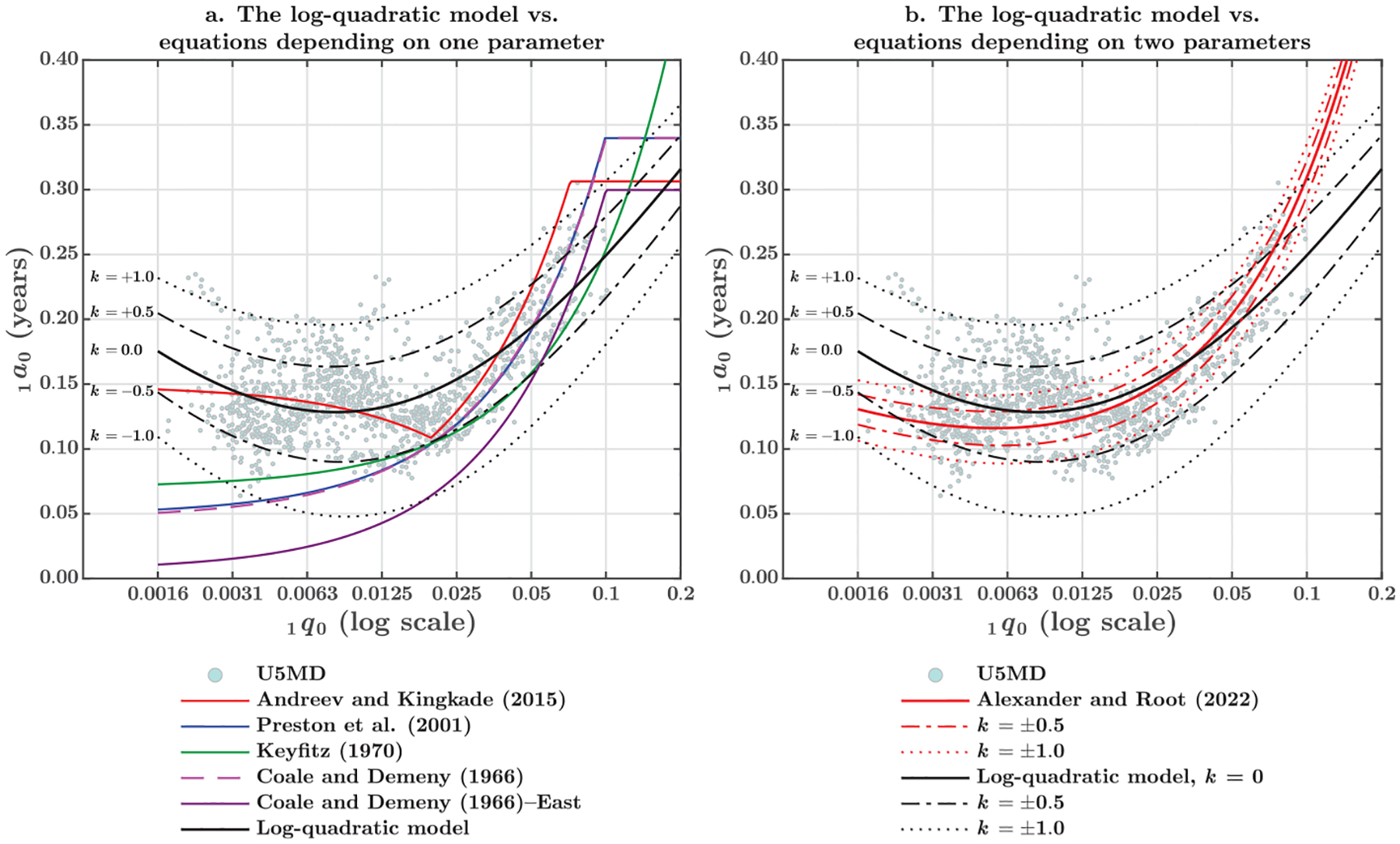
The average age of infant deaths, , as a function of the probability of dying within the first year of life, described by classic and new approaches (both sexes combined). Keyfitz (1970) proposed only one general formula for both sexes; Andreev and Kingkade (2015), Preston et al. (2001), and Coale and Demeny (1966) did not report equations for both sexes combined. Average coefficients were calculated for comparability purposes, assuming a sex ratio at birth of 1.05 males per female. The other methods estimate coefficients for males, females, and both sexes combined, which are more precise than applying an SRB.
In addition to the predicted values of , Figure 1 shows the empirical values of 1,219 country-years from the U5MD directly estimated, as explained in the Data section, and the indirect estimation of the log-quadratic model—given five values of that represent different age patterns of under-five mortality. Panel a makes evident the contribution of Andreev and Kingkade (2015) of avoiding a monotonic function that has no empirical support at very low levels of infant mortality. Although the segmented AK formula incorporates a modest increase in the average age of infant deaths, is overdispersed at low levels of infant mortality and predictions based on alone are not precise. Conversely, the log-quadratic model has the flexibility to move from the central tendency by adjusting the value of . A combination of and increases the accuracy in estimating the average age of infant deaths , but fitting the log-quadratic requires some knowledge or inference on the value of .
Panel b of Figure 1 compares the new formula proposed by Alexander and Root in 2022 (hereafter AR) with the indirect estimation of the log-quadratic model. Since these two approaches include more than one parameter, the estimated value of should be specific to a given age pattern of under-five mortality. While the log-quadratic model is a system of equations depending on the level of the under-five mortality and the value of , AR’s equation is a direct equation regressing the average age of infant deaths on the probability of dying during the first year of life and the ratio of this probability to the under-five mortality. To make these two approaches comparable, AR’s equation has been plotted to indicate the same range of values of (i.e., the same variation of the age pattern). For a given pair of and , the corresponding value of the under-five mortality is calculated by matching the log-quadratic model to this information. As shown in the following section (see Figure 3), there is only one value of for a given pair of and , thus ensuring a unique solution. Finally, is estimated from and , using the AR’s ratio equation and plotting against the chosen level of .
Fig. 3.
Contour lines representing the different combinations of and that result in the same value of a mortality function, given the coefficients of the log-quadratic model (both sexes combined)
Panel b of Figure 1 also shows that AR’s formula is not covering the full range of variation of the mean age of infant deaths, given the expected variation in and the level of infant mortality. The most likely explanation is that and —as well as and —is not an ideal combination for inferring the age pattern of under-five mortality. Indeed, the level of the under-five mortality is strongly determined by the value of the infant mortality, and the ratio of the infant to the under-five mortality is not strongly correlated with the average age of infant deaths. Hence, to improve on the estimation of the average age of infant deaths, the researcher must rely on inputs that better inform the age distribution of deaths during the first year of life.
The same inputs of can be used to estimate the average number of years lived—in the age interval—by those dying during childhood. Although is also a necessary component of an abridged life table, its empirical validation has received less attention. In addition to the formulae proposed by Coale and Demeny (1966), imposing a value of 1.5 years has been used as a raw assumption (Keyfitz and Flieger 1971), disregarding the level and the age pattern of mortality. One of the reasons might be the lesser influence of this value on the resulting under-five mortality rate.
Figure 2 shows observed and predicted values of as a function of the infant mortality rate. Panel a illustrates the four regional families of mortality (i.e., North, South, West, and East) initially proposed by Coale and Demeny (1966); the alternative West formula by Preston et al. (2001), depending on ; and the predictions of the log-quadratic model of under-five mortality for five given values of . Panel b emphasizes the flexibility of the model and the effect of modifying the age patterns at different levels of mortality. Figure 2 also shows that the classic approach is only partially supported by the empirical data, and there are important gaps between one regional family and the other. Assuming 1.5 years is not unrealistic but sacrifices accuracy and precision. As in the case of the average age of infant deaths, the graduation of improves the estimation of , when the researcher relies on the log-quadratic model. In addition to the flexibility, one advantage of the log-quadratic model is to show a modest reduction in the estimated value of at very low levels of mortality, where child deaths tend to concentrate more at the beginning of the age interval.
Fig. 2.

The average number of years lived—in the age interval—by those dying during childhood, , as a function of the probability of dying within the first year of life, described by classic and new approaches (both sexes combined). Preston et al. (2001) and Coale and Demeny (1966) did not report equations for both sexes combined. Average coefficients were calculated for comparability purposes, assuming a sex ratio at birth of 1.05 males per female.
Optimal Values of and , Matching the Model to Observed Data
Model estimates—denoted as a function of and —implicitly assume that the researcher knows the value of the parameters. Considering that these parameters might not be directly observed quantities, they can be recovered by fitting the model to some observed inputs (Guillot et al. 2022a). In this article, our proposal is to find the optimal values of and by adapting a log-quadratic model to reproduce exactly one or two observed inputs: for example, central death rates and the age distribution of infant deaths, when the latter is available. Following the same principle as Eqs. (3) and (4), death rates—depending on the estimated number of deaths and the number of person-years lived between ages and —can be calculated with
| (5) |
Given two key assumptions of the log-quadratic model of under-five mortality (i.e., constant force of mortality within the age subinterval and proportional exposure to the length of each subinterval of age), the observed proportion of infant deaths below a certain age —denoted by —can be calculated by
| (6) |
Since the proportion of infant deaths from 0 to age depends exclusively on the probability of dying below the same age and the infant mortality rate, knowing just two of these quantities is enough to calculate the one that would be missing, as indicated by Eq. (6). This condition facilitates some applications, inasmuch as the age distribution of infant deaths is more available than the actual probabilities of dying, and researchers can use the proportion of infant deaths below a certain age as one of the inputs to graduate the values of and .
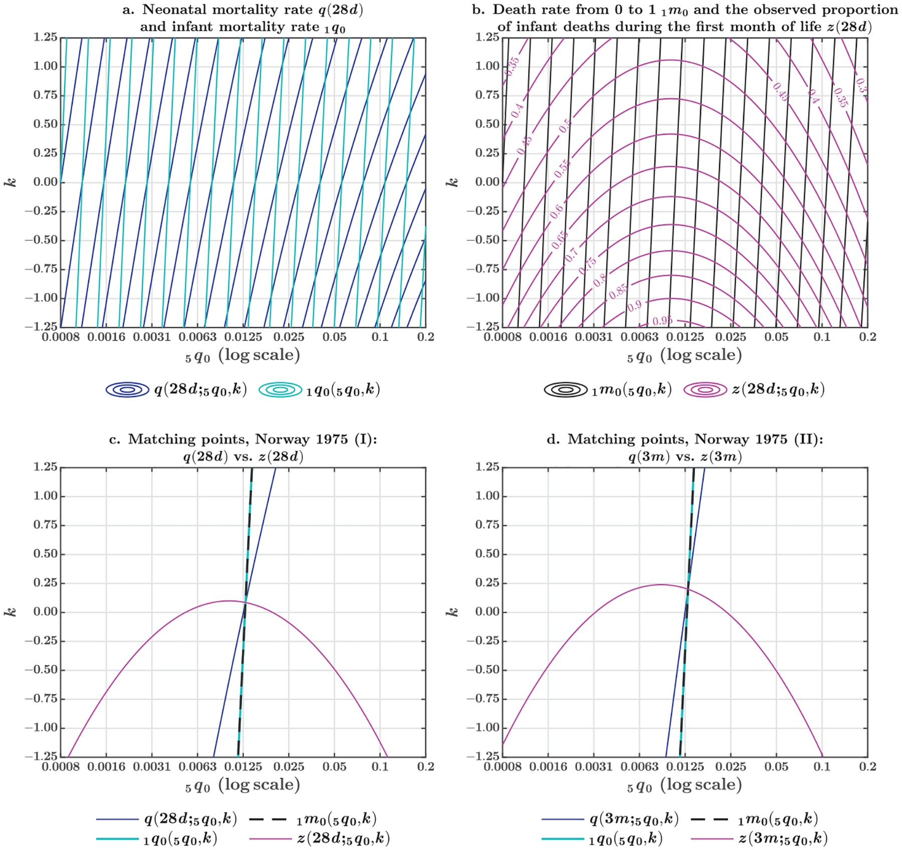
Let us first describe a graphical solution to the problem of matching Eqs. (5) and (6). Using the coefficients of the log-quadratic model , Figure 3 shows contour lines representing the different combinations of and that will result in the same value of some mortality inputs. Therefore, the model is matching the observed values of two inputs at the exact point in which their corresponding lines intersect. The optimal solutions of the log-quadratic model exist along these intersections. If the contour lines intersect only once, the precise combination of and is also unique. Some combinations of mortality inputs lead to unique solutions of the model; Figure 3 is illustrating just a couple of them.
On the one hand, panel a of Figure 3 shows the contour lines of the neonatal mortality rate (in dark blue) and the infant mortality rate (in light blue), generated using the outcomes of Eq. (2). On the other hand, panel b depicts the contour lines of the central death rate from 0 to 1 (in dark gray) and the proportion of infant deaths during the first month of life (in pink), generated using Eqs. (5) and (6), respectively. These two combinations produce equivalent solutions, as shown in panel c, using Norway in 1975 as an example.
At the exact point that the model is matching the neonatal mortality rate and the infant mortality rate , the model is also matching the death rate from 0 to 1, , and the proportion of infant deaths during the first month of life, , as suggested by Eq. (6). In addition, given the assumptions of the log-quadratic model, the contours of and describe overlapping solutions. Although these two mortality inputs have different numeric values, they imply the same combination of parameters and . Thus, matching would be equivalent to matching , when the first quantity is more available. Finally, panel d of Figure 3 demonstrates the same property when the log-quadratic model is matching the probability of dying during the first three months of life , or the equivalent solution when the proportion of infant deaths during the first trimester of life is more available.
Now, let us formulate the analytical solution to the problem of matching. Finding the combinations of parameters and requires solving a system of two nonlinear equations. Let us assume that the researcher is matching the log-quadratic model to the observed death rate from 0 to 1—indicated by —and the observed proportion of infant deaths during the first trimester of life—denoted by . As shown in this article, these two inputs can be estimated at a given level and age pattern of under-five mortality using Eqs. (2), (4), (5), and (6). Then, the researcher can define the functions and as the residual of the model when trying to predict the natural logarithm of each observed input, as proposed by Eqs. (7.1) and (7.2):
| (7.1) |
| (7.2) |
Then, the optimal values of and are calculated by successive approximations, as the residual of the log-quadratic model approaches zero in both cases. Using the Newton–Raphson method and starting from an arbitrary—but feasible—choice (i.e., is positive but less than one; and is equal to zero), these two parameters can be iterated from Eq. (8), until convergence is reached:
| (8) |
When the log-quadratic model is matching only one input, some specific value of must be assumed. We recommend using a distribution of values, but if no prior information is available, is characterizing the neutral or average age pattern of under-five mortality that is implicit in the log-quadratic model. Finally, the average age of infant deaths and the average number of years lived—in the age interval—by those dying during childhood are calculated by Eq. (3), using the unique mortality schedule produced by the optimal values of and . To facilitate its implementation, the method has been written as a computer application and two worked examples are described step-by-step in online appendix 1.
Evaluation
To evaluate the performance of our method, we fit the log-quadratic model to each country-year of the U5MD and compute the error of predicting either or —matching one or two inputs. We then estimate the accuracy and precision, assuming that these residuals are the result of a systematic bias and a measurement error , whose expected value is zero and variance is equal to , as indicated by Eq. (9) for any country-year :
| (9) |
While is indicative of the lack of accuracy, the value of is informing the precision when the log-quadratic model is matching specific inputs. Then, we use these values to calculate the root mean square error (RMSE)—as defined by Eq. (10)—which is one conventional metric to evaluate the overall predictive power of mortality models:
| (10) |
Following a Bayesian framework, measures of accuracy, precision, and predictive power are estimated for each sex, for both sexes combined, and for different combinations of inputs. The advantage of the Bayesian analysis is to equip each model with the corresponding credible intervals that are useful for comparisons, as described in online appendix 2. We extend this analysis to all previous approaches that have been proposed to approximate the values of and . As the error of prediction is the main input of Eq. (9), the coefficients of these previous approaches were not reestimated in this article. We simply calculate the error of predicting and from the observed values of or —and in the case of AR’s formula—using the parameters reported by these previous studies. Credible intervals were also calculated for these approaches, using the same prior distributions to fit Eq. (9).
To this list of competing approaches, we add two equations resulting from a linear regression of on the best predictors of the age patterns of under-five mortality that we identify in this article: and . The details of this regression approach are discussed in online appendix 3.
Results
The Average Age of Infant Deaths
Table 2 reports the accuracy, precision, and predictive power of the log-quadratic model, compared with the competing approaches to estimate the average age of infant deaths. Reported values correspond to the percentiles 50, 2.5, and 97.5, sampling the conditional posterior distributions of the bias and the precision and calculating the resulting RMSE for each sample. Those approaches using two inputs are grouped at the top of the table and those using only one input are at the bottom. The table shows that matching two inputs reduces the bias and increases the precision of the log-quadratic model. This is particularly the case of inputs informing the concentration of deaths during the first weeks or months of life, which is a proxy of the age patterns of under-five mortality. The same result is found for each sex and for both sexes combined.
Table 2.
Bias, precision, and the root mean square error (RMSE) of predicting the average age of infant deaths, , and fitting different methods to the Under-5 Mortality Database
| Female | Male | Both Sexes Combined | |||||||
|---|---|---|---|---|---|---|---|---|---|
| (bias) | (precision) | RMSE | (bias) | (precision) | RMSE | (bias) | (precision) | RMSE | |
| A. Log-Quadratic Model, and | −0.0019 [−0.0046, 0.0009] |
432.72 [399.18, 468.14] |
0.0481 [0.0463, 0.0501] |
−0.0023 [−0.0048, 0.0004] |
486.64 [448.92, 526.48] |
0.0454 [0.0437, 0.0473] |
−0.0016 [−0.0037, 0.0005] |
743.57 [685.95, 804.45] |
0.0367 [0.0353, 0.0382] |
| B. Log-Quadratic Model, and | 0.0006 [−0.0037, 0.0050] |
163.43 [150.60, 176.79] |
0.0783 [0.0752, 0.0815] |
−0.0011 [−0.0054, 0.0032] |
169.74 [156.42, 183.63] |
0.0768 [0.0738, 0.0800] |
−0.0010 [−0.0048, 0.0028] |
215.24 [198.35, 232.84] |
0.0682 [0.0656, 0.0710] |
| C. Log-Quadratic Model, and | −0.0111 [−0.0248, 0.0025] |
17.00 [15.68, 18.38] |
0.2429 [0.2336, 0.2529] |
−0.0160 [−0.0311, −0.0012] |
14.16 [13.06, 15.31] |
0.2664 [0.2562, 0.2774] |
−0.0119 [−0.0250, 0.0010] |
18.74 [17.29, 20.27] |
0.2314 [0.2225, 0.2409] |
| D. Log-Quadratic Model, and | −0.0111 [−0.0246, 0.0028] |
17.07 [15.74, 18.44] |
0.2424 [0.2331, 0.2523] |
−0.0161 [−0.0309, −0.0008] |
14.22 [13.12, 15.37] |
0.2657 [0.2556, 0.2766] |
−0.0119 [−0.0248, 0.0013] |
18.84 [17.38, 20.36] |
0.2308 [0.2220, 0.2402] |
| E. Alexander and Root (2022), and, | −0.0570 [−0.0683, −0.0460] |
26.21 [24.18, 28.35] |
0.2036 [0.1957, 0.2118] |
−0.0492 [−0.0612, −0.0375] |
23.03 [21.25, 24.92] |
0.2141 [0.2060, 0.2230] |
−0.0507 [−0.0617, −0.0400] |
27.63 [25.49, 29.89] |
0.1969 [0.1894, 0.2050] |
| F. Linear Regression, | 0.0007 [−0.0021, 0.0035] |
399.25 [368.19, 431.93] |
0.0501 [0.0481, 0.0521] |
0.0005 [−0.0022, 0.0032] |
428.12 [394.82, 463.16] |
0.0484 [0.0465, 0.0503] |
0.0004 [−0.0019, 0.0026] |
622.90 [574.45, 673.89] |
0.0401 [0.0385, 0.0417] |
| G. Linear Regression, | 0.0020 [−0.0028, 0.0067] |
141.63 [130.57, 153.14] |
0.0841 [0.0809, 0.0876] |
0.0015 [−0.0032, 0.0061] |
148.98 [137.34, 161.09] |
0.0820 [0.0788, 0.0854] |
0.0011 [−0.0032, 0.0052] |
178.78 [164.81, 193.31] |
0.0748 [0.0720, 0.0780] |
| H. Log-Quadratic Model, and | 0.0278 [0.0161, 0.0395] |
22.78 [21.05, 24.64] |
0.2115 [0.2034, 0.2200] |
0.0307 [0.0185, 0.0428] |
21.19 [19.59, 22.92] |
0.2195 [0.2111, 0.2283] |
0.0271 [0.0157, 0.0385] |
23.95 [22.14, 25.91] |
0.2062 [0.1983, 0.2145] |
| I. Log-Quadratic Model, and | 0.0278 [0.0161, 0.0394] |
22.74 [20.96, 24.56] |
0.2116 [0.2036, 0.2203] |
0.0306 [0.0186, 0.0427] |
21.15 [19.50, 22.85] |
0.2197 [0.2113, 0.2287] |
0.0271 [0.0157, 0.0384] |
23.91 [22.04, 25.83] |
0.2064 [0.1986, 0.2149] |
| J. Log-Quadratic Model, and | 0.0274 [0.0158, 0.0393] |
22.67 [20.91, 24.50] |
0.2119 [0.2040, 0.2207] |
0.0302 [0.0182, 0.0426] |
21.09 [19.44, 22.78] |
0.2200 [0.2118, 0.2291] |
0.0267 [0.0154, 0.0383] |
23.82 [21.97, 25.74] |
0.2067 [0.1991, 0.2153] |
| K. Andreev and Kingkade (2015), | 0.0032 [−0.0085, 0.0150] |
22.60 [20.87, 24.39] |
0.2105 [0.2026, 0.2190] |
0.0155 [0.0035, 0.0275] |
21.84 [20.18, 23.58] |
0.2146 [0.2065, 0.2233] |
0.0125
[0.0012, 0.0239] |
24.33
[22.48, 26.26] |
0.2032
[0.1956, 0.2114] |
| L. Preston et al. (2001), | −0.4828 [−0.5012, −0.4638] |
9.30 [8.59, 10.07] |
0.5837 [0.5664, 0.6009] |
−0.4526 [−0.4757, −0.4287] |
5.86 [5.41, 6.35] |
0.6128 [0.5919, 0.6340] |
−0.4646 [−0.4852, −0.4433] |
7.39
[6.83, 8.00] |
0.5927
[0.5736, 0.6117] |
| M. Keyfitz (1970), | −0.4368 [−0.4499, −0.4234] |
18.03
[16.62, 19.45] |
0.4963
[0.4840, 0.5090] |
−0.3283 [−0.3439, −0.3126] |
12.94
[11.93, 13.96] |
0.4303
[0.4170, 0.4445] |
−0.3798 [−0.3938, −0.3657] |
15.95 [14.71, 17.21] |
0.4550 [0.4424, 0.4683] |
| N. Coale and Demeny (1966), | −0.5000 [−0.5188, −0.4811] |
8.61 [7.95, 9.33] |
0.6052 [0.5880, 0.6230] |
−0.4634 [−0.4869, −0.4399] |
5.53 [5.11, 5.99] |
0.6290 [0.6082, 0.6506] |
−0.4784 [−0.4994, −0.4573] |
6.90
[6.36, 7.47] |
0.6115
[0.5927, 0.6313] |
| O. Coale and Demeny (1966)—East, | −1.2131 [−1.2475, −1.1791] |
2.68 [2.47, 2.89] |
1.3586 [1.3267, 1.3910] |
−1.2474 [−1.2928, −1.2026] |
1.54 [1.42, 1.66] |
1.4855 [1.4443, 1.5271] |
−1.2220 [−1.2617, −1.1828] |
2.01
[1.85, 2.17] |
1.4110
[1.3746, 1.4478] |
Notes: Values are the median of the posterior probability distribution and the 2.5th and 97.5th percentiles. Andreev and Kingkade (2015), Preston et al. (2001), and Coale and Demeny (1966) did not report equations for both sexes combined. For these entries, average coefficients were calculated for comparability purposes, assuming a sex ratio at birth of 1.05 males per female. Keyfitz (1970) proposed only one general formula for both sexes combined. Resulting values of these approaches are shown in italics.
Less conventional indicators can be good predictors of . The proportion of infant deaths during the first trimester —or the first month of life —improves the predictive power of the log-quadratic model if used together with the infant mortality rate—or the central death rate from 0 to 1. As described by rows A and B, when the log-quadratic model is matching the observed values of or , the bias is not significant and the precision reaches its maximum, compared with an alternative solution relying on alone, as seen in row I (RMSE is 0.0367 when adding vs. 0.2064 for alone). Indeed, the improvement of the log-quadratic model—by means of an indirect estimation—outperforms the competing approaches to estimate the average age of infant deaths.
Because of the relevance of the neonatal deaths, can be more available than . However, as shown in Table 2, the latter is considerably more precise in predicting the average age of infant deaths (0.0682 vs. 0.0367 for the RMSE). This result holds for indirect estimations—contrasting the models of rows A and B—and for direct estimations—comparing the linear regressions of rows F and G.
Nonetheless, the indirect estimation of is fully supported by the empirical data, and the log-quadratic model is more precise than the regression counterparts when using either or . This comparison should take into consideration that linear regressions might be affected by overfitting, while the coefficients of the log-quadratic model were not estimated with the aim to predict the observed value of . As shown in Table 2 for both sexes combined, indirect estimations described in rows A and B are significantly better than the linear regressions in rows F and G (i.e., credible intervals of precision do not overlap). However, when comparing the same rows for the male and the female populations individually, the superiority of the log-quadratic model is retained, but it is not statistically significant at 5% (i.e., credible intervals overlap).
Although and —or and —do reduce the bias of the log-quadratic model as suggested by the comparison of rows C and H—or rows D and I—this is not an ideal combination of inputs for predicting as the value of the precision decreases. Hence, to effectively increase the predictive power of the indirect estimation, better inputs should inform the age pattern of under-five mortality. If is available, the list of complementary inputs should include the observed neonatal mortality rate , the probability of dying during the first trimester of life , or the proportions and that are leading to equivalent solutions of the log-quadratic model. Therefore, if these inputs are not available, the most conservative selection would be to match only one input, assuming a predefined value of —as reported in rows H, I, and J.
Indeed, matching just one input is not an ideal solution but it does not diminish the predictive power of the log-quadratic model—if compared to the competing approaches. When the model matches the infant mortality rate , the central death rate from 0 to 1 , or that from 0 to 5 , the resulting RMSE is not statistically different from the one produced by the ratio equation proposed by Alexander and Root (2022) with two inputs—described in row E—or the segmented equation estimated by Andreev and Kingkade (2015) for one input—given in row K of Table 2. Nevertheless, as an advantage inherited from the log-quadratic model, the accuracy might be improved by using external information regarding the likely value of . For simplicity, the models reported in rows H, I, and J assume a neutral—or average—age pattern of under-five mortality represented by , which is a neutral approximation when the age pattern of under-five mortality cannot be inferred from the data. However, in practical applications taking advantage of the flexibility of the log-quadratic model, researchers can either draw a full distribution of the feasible values of or assume only positive values—or negative values—a priori if the population under investigation is more likely to have late—or early—age patterns of under-five mortality, as informed by another reliable source (e.g., a demographic survey).
Table 2 shows that classic approaches—Preston et al. (2001), Keyfitz (1970), and Coale and Demeny (1966), reported in rows L, M, N, and O—are significantly biased and return low precision when predicting the average age of infant deaths informed by the U5MD. This result is driven by the lack of fitting at low levels of infant mortality (e.g., fewer than 20 deaths per thousand births), previously shown in Figure 1. Considering this limitation, classic approaches are less recommended and, if used, these methods should be implemented with extra precaution and only for admissible levels of infant mortality. A graphical analysis of the main results is described in the online appendix.
The Average Number of Years Lived—in the Age Interval—by Those Dying From 1 to 5,
Table 3 reports the predictive power of the log-quadratic model when estimating indirectly. The table compares the bias and precision of matching one or two inputs—in rows A to G—with the classic approaches of Preston et al. (2001), Keyfitz and Flieger (1971), and Coale and Demeny (1966)—described in rows H to M. Contrary to the case for , the different methods to estimate do not vary too much in terms of accuracy and precision.
Table 3.
Bias, precision, and the root mean square error (RMSE) of predicting the average number of years lived—in the age interval—by those dying between ages 1 and 5, , and fitting different methods to the Under-5 Mortality Database
| Female | Male | Both Sexes Combined | |||||||
|---|---|---|---|---|---|---|---|---|---|
| (bias) | (precision) | RMSE | (bias) | (precision) | RMSE | (bias) | (precision) | RMSE | |
| A. Log-Quadratic Model, , and | 0.0074 [0.0024, 0.0127] |
122.76 [113.24, 132.81] |
0.0906 [0.0871, 0.0943] |
0.0066 [0.0023, 0.0110] |
169.29 [156.17, 183.15] |
0.0772 [0.0742, 0.0803] |
0.0054 [0.0017, 0.0093] |
225.02 [207.59, 243.45] |
0.0669 [0.0644, 0.0696] |
| B. Log-Quadratic Model, and | 0.0072 [0.0022, 0.0123] |
122.50 [112.89, 132.51] |
0.0907 [0.0872, 0.0945] |
0.0065 [0.0022, 0.0109] |
166.05 [153.02, 179.63] |
0.0779 [0.0749, 0.0812] |
0.0055 [0.0017, 0.0092] |
222.18 [204.75, 240.35] |
0.0673 [0.0648, 0.0701] |
| C. Log-Quadratic Model, and | 0.0078 [0.0026, 0.0130] |
116.09 [107.07, 125.54] |
0.0932 [0.0896, 0.0970] |
0.0074 [0.0028, 0.0120] |
150.07 [138.41, 162.29] |
0.0820 [0.0788, 0.0854] |
0.0059 [0.0019, 0.0098] |
201.49 [185.84, 217.90] |
0.0707 [0.0680, 0.0737] |
| D. Log-Quadratic Model, and | 0.0078 [0.0026, 0.0131] |
116.02 [107.03, 125.39] |
0.0932 [0.0896, 0.0971] |
0.0074 [0.0028, 0.0121] |
149.96 [138.35, 162.08] |
0.0820 [0.0789, 0.0854] |
0.0059 [0.0020, 0.0099] |
201.30 [185.71, 217.57] |
0.0708 [0.0680, 0.0737] |
| E. Log-Quadratic Model, and | 0.0034 [−0.0017, 0.0085] |
119.16 [110.12, 128.89] |
0.0917 [0.0882, 0.0954] |
0.0020 [−0.0024, 0.0065] |
157.44 [145.50, 170.29] |
0.0798 [0.0767, 0.0830] |
0.0016 [−0.0023, 0.0054] |
210.21 [194.28, 227.38] |
0.0690 [0.0664, 0.0718] |
| F. Log-Quadratic Model, and | 0.0034 [−0.0017, 0.0085] |
119.03 [109.74, 128.58] |
0.0918 [0.0883, 0.0956] |
0.0020 [−0.0024, 0.0065] |
157.23 [144.95, 169.85] |
0.0798 [0.0768, 0.0831] |
0.0016 [−0.0023, 0.0054] |
209.94 [193.54, 226.78] |
0.0691 [0.0665, 0.0719] |
| G. Log-Quadratic Model, and | 0.0036 [−0.0015, 0.0088] |
117.89 [108.71, 127.36] |
0.0922 [0.0888, 0.0960] |
0.0022 [−0.0022, 0.0068] |
154.70 [142.67, 167.14] |
0.0805 [0.0774, 0.0838] |
0.0018 [−0.0021, 0.0057] |
205.52 [189.54, 222.04] |
0.0698 [0.0672, 0.0727] |
| H. Preston et al. (2001), | −0.0246 [−0.0300, −0.0193] |
109.59 [101.04, 118.47] |
0.0987 [0.0950, 0.1028] |
0.0031 [−0.0015, 0.0077] |
146.64 [135.21, 158.53] |
0.0827 [0.0795, 0.0861] |
−0.0121 [−0.0162, −0.0080] |
187.29
[172.68, 202.46] |
0.0741
[0.0713, 0.0771] |
| I. Keyfitz and Flieger (1971), | −0.0230 [−0.0287, −0.0173] |
97.04
[89.65, 104.74] |
0.1041
[0.1002, 0.1083] |
−0.0568 [−0.0621, −0.0515] |
110.22
[101.82, 118.97] |
0.1109
[0.1069, 0.1153] |
−0.0434 [−0.0481, −0.0387] |
139.77 [129.12, 150.87] |
0.0951 [0.0916, 0.0988] |
| J. Coale and Demeny (1966)—North, | 0.1065 [0.1012, 0.1121] |
108.34 [100.11, 117.34] |
0.1435 [0.1388, 0.1485] |
0.1248 [0.1201, 0.1296] |
144.09 [133.14, 156.06] |
0.1501 [0.1458, 0.1546] |
0.1140
[0.1099, 0.1183] |
182.70
[168.81, 197.87] |
0.1359
[0.1321, 0.1399] |
| K. Coale and Demeny (1966)—South, | −0.0490 [−0.0544, −0.0437] |
110.05 [101.45, 118.74] |
0.1072 [0.1033, 0.1116] |
−0.0217 [−0.0264, −0.0171] |
146.80 [135.33, 158.40] |
0.0854 [0.0822, 0.0889] |
−0.0367 [−0.0408, −0.0326] |
188.43
[173.70, 203.31] |
0.0816
[0.0786, 0.0849] |
| L. Coale and Demeny (1966)—West, | −0.0240 [−0.0293, −0.0187] |
109.72 [101.25, 118.86] |
0.0985 [0.0946, 0.1026] |
0.0031 [−0.0015, 0.0076] |
146.37 [135.06, 158.56] |
0.0828 [0.0795, 0.0862] |
−0.0118 [−0.0158, −0.0077] |
187.41
[172.94, 203.02] |
0.0740
[0.0711, 0.0771] |
| M. Coale and Demeny (1966)—East, | −0.1090 [−0.1143, −0.1037] |
110.72 [102.00, 119.60] |
0.1446 [0.1400, 0.1494] |
−0.0699 [−0.0745, −0.0653] |
147.44 [135.84, 159.27] |
0.1081 [0.1042, 0.1120] |
−0.0903 [−0.0944, −0.0863] |
190.41
[175.43, 205.68] |
0.1158
[0.1123, 0.1195] |
Notes: Values are the median of the posterior probability distribution and the 2.5th and 97.5th percentiles. Preston et al. (2001) and Coale and Demeny (1966) did not report equations for both sexes combined. For these entries, average coefficients were calculated for comparability purposes, assuming a sex ratio at birth of 1.05 males per female. Keyfitz and Flieger (1971) proposed only one general approximation for any human population. Resulting values of these approaches are shown in italics.
Matching two inputs does increase the predictive power of the log-quadratic model, yet the improvement is not always statistically significant, even if the inputs inform the age patterns of under-five mortality: for example, when the fitting of the model reported in row A or B is compared to the counterpart of the model reported in row F. However, when the log-quadratic model is matching either or —and minimizing the prediction error of —the resulting RMSE of predicting is significantly lower than that produced by any classic approach. Hence, the log-quadratic model would provide the best possible solution for as a by-product of estimating the average age of infant deaths.
Table 3 shows that a constant value of 1.5 years—as proposed by Keyfitz and Flieger (1971)—has some empirical support, but it might be a crude assumption and, evidently, not the best choice when researchers are looking for some precision. The formula adapted by Preston et al. (2001) produces virtually the same results of the West model of mortality, initially proposed by Coale and Demeny (1966). Although the West model has an adequate fitting to the U5MD, the predictive power of the other regional families is limited by the significant bias. This result is partially driven by the nature of the classic method to represent the diversity of patterns of mortality using four regional families. Hence, any practical application of the classic method requires an expert opinion on the age pattern to inform the appropriate family to estimate .
Discussion
This article proposes a new method for estimating the average age of infant deaths by using a model life table of under-five mortality by detailed age that brings greater flexibility and precision, compared with existing approaches that deal with generic equations and fixed inputs. Because the model depends on one or two parameters—related to the level and the age pattern of mortality at early ages—the aim of the method is to find the value of these parameters by fitting or matching the model life table to some observed data. Hence, the average age of infant deaths can be estimated indirectly for a given value of one or two available inputs that can be either death rates, probabilities of dying, or the proportion of deaths during the first months of life.
Because this method relies on a model life table, other mortality indicators can also be calculated, simultaneously, at no extra effort: for example, the average number of years lived—in the age interval—by those dying during childhood , which is a necessary value to estimate the under-five mortality rate , when the death rates from 0 to 1 and from 1 to 5 are used as inputs. Moreover, the same principle is extended to less conventional but necessary parameters, such as the average age of under-five deaths , which mediates the calculation of the under-five mortality rate when the central death rate from 0 to 5 years is the only information available. The flexibility and the completeness of our method contrast with the existing equations to estimate or separately, as well as with those approaches that simply do not propose a solution for estimating , such as Andreev and Kingkade (2015) or Alexander and Root (2022).
This article shows that accounting for the age pattern of mortality does improve the estimation of the average age of infant deaths and the average number of years lived—in the age interval—by those dying during childhood. Although the foundational work of Coale and Demeny (1966) made a relevant distinction of the age patterns of mortality to estimate the values of and , both classic and new approaches have proposed generic equations that depend only on the level of mortality and lead to large errors of prediction. Our method departs from these approaches, considering that, at the same level of mortality, infant deaths can be relatively more (or less) concentrated during the first months of life, thus producing different values of .
Inferring the right pattern requires inputs that inform the compression of deaths during the first weeks and months of life, relative to the overall level of infant (or under-five) mortality. Not all inputs are equally effective for this purpose. In one of the most recent approaches to estimate the average age of infant deaths, Alexander and Root (2022) proposed the ratio of infant to under-five mortality rate as a secondary input. However, and are highly correlated at the population level and the ratio is not a strong predictor of the age distribution of deaths during the first year of life. We show that easily accessible indicators, such as the neonatal mortality or the proportion of infant deaths during the first months of life, add more precision and effectively minimize the prediction error of and , and so produce better results than any existing approach.
Although these indicators are not yet available in key repositories such as the Human Mortality Database, the WHO Mortality Database, or the Human Life-Table Database, both the number of neonatal deaths and the age distribution of infant deaths have been reported by some statistical yearbooks for more than a hundred years and disseminated by the Demographic Yearbook of the United Nations since 1948 and 1967, respectively (United Nations 1949, 1968). In some applications, however, the age distribution of infant deaths might not be available or reliable (e.g., in historical populations or those with incomplete vital registration systems). If that is the case, we recommend matching the log-quadratic model to only one input that will inform the overall level of under-five mortality at a predefined value of . By assuming a neutral age pattern of mortality (i.e., ), the performance of the method would be similar to the most recent approaches using direct estimations, such as the one-parameter formula of Andreev and Kingkade (2015) or the two-parameter formula proposed by Alexander and Root (2022). Nevertheless, the researcher applying our method will have the advantage of setting one or more values of , as supported by an expert opinion or for the sake of sensitivity analysis.
Our method builds on the estimated coefficients of a log-quadratic model applied to the U5MD—describing a broad range of age patterns of under-five mortality (Guillot et al. 2022a). Applications have shown a satisfactory fitting of the log-quadratic model to a broad set of populations in low- and middle-income countries that were not included in the U5MD, except for sub-Saharan African and South Asian populations (Romero Prieto et al. 2021; Verhulst et al. 2022). In these two regions, the age patterns of under-five mortality are different from those observed in the U5MD (i.e., from the age patterns observed in the historical experience of high-income countries), but this limitation affects all the existing methods—all based on high-quality vital records data—that we have compared in this article. Nonetheless, the log-quadratic model and its higher flexibility for estimating and can be updated with data from other populations. Therefore, to apply our method to sub-Saharan African and South Asian populations, we recommend using a different set of coefficients that best represent the age patterns of under-five mortality in these populations.
There might exist a trade-off between evaluating a direct formula—following any of the existing approaches—and adjusting a model life table to calculate the average age of infant deaths, as we propose. While evaluating a single equation is computationally inexpensive, adjusting a model life table to fit one or two inputs requires few iterations. Given that the existing approaches—depending on or alone—yield coarse approximations for the actual value of , our method reaches greater precision at a reasonable computational cost (e.g., implementing the software that is associated with this article). Indeed, if a simple equation were meant to be used to predict , that formula should depend on the percentage of infant deaths during the first three months of life. However, despite the great linear fitting, this input does not reach the same precision and flexibility of the method that we propose.
Conclusion
The average age of infant deaths, , is properly estimated by a model life table of under-five mortality. Contrary to the previous approaches based on a single formula, fitting—or matching—a model to some observed data has three clear advantages: (1) the flexibility to describe a broad range of age patterns of under-five mortality; (2) the adaptability to incorporate a variety of inputs for indirect estimation (e.g., mortality rates, probabilities of dying, or the proportion of infant deaths during the first months of life); and (3) the extensibility to other essential parameters for life table construction, such as the average number of years lived—in the age interval—by those dying during childhood, , and the average age of under-five deaths, . Accounting for the age patterns of under-five mortality improves the estimation of the average age of infant deaths when a direct calculation is not possible, which is the case for aggregated data that are simply tabulated by years of age.
The accuracy of the method depends on inferring the actual age pattern of under-five mortality, but not all inputs are adequate for this indirect estimation. One suitable combination of inputs is the infant mortality rate and a probability of dying during the first months of life (e.g., the neonatal mortality rate or the probability of dying during the first trimester of life). An equivalent solution can be reached using alternative and easily accessible inputs, such as the central death rate from 0 to 1 and the proportion of infant deaths below a certain age. Hence, life table construction can benefit from the indirect estimation of the average age of infant deaths and the average number of years lived—in the age interval—by those dying during childhood by using some information related to the age distribution of deaths during the first year of life. ■
Supplementary Material
Acknowledgments
Research reported in this article was supported by the Eunice Kennedy Shriver National Institute of Child Health and Human Development of the National Institutes of Health (award R01HD090082). Early versions of this work were presented at the 2021 annual meetings of the Population Association of America (Mathematical Demography), the British Society for Population Studies (Health and Mortality: Child and Adolescent Health), and IUSSP-IPC (Creating and Using International or Historical Datasets).
Footnotes
ELECTRONIC SUPPLEMENTARY MATERIAL The online version of this article (https://doi.org/10.1215/00703370-11330227) contains supplementary material.
Contributor Information
Julio Romero-Prieto, Department of Population Health, London School of Hygiene and Tropical Medicine, London, UK.
Andrea Verhulst, Institut National d’Études Démographiques, Aubervilliers, France.
Michel Guillot, Population Studies Center, University of Pennsylvania, Philadelphia, PA, USA; Institut National d’Études Démographiques, Aubervilliers, France.
References
- Alexander M, & Root L (2022). Competing effects on the average age of infant death. Demography, 59, 587–605. 10.1215/00703370-9779784 [DOI] [PubMed] [Google Scholar]
- Andreev EM, & Kingkade WW (2015). Average age at death in infancy and infant mortality level: Reconsidering the Coale-Demeny formulas at current levels of low mortality. Demographic Research, 33, 363–390. 10.4054/DemRes.2015.33.13 [DOI] [Google Scholar]
- Arias E, & Xu J (2019). United States life tables, 2017 (National Vital Statistics Reports, Vol. 68 No.7). Hyattsville, MD: National Center for Health Statistics. Retrieved from https://www.cdc.gov/nchs/data/nvsr/nvsr68/nvsr68_07-508.pdf [PubMed] [Google Scholar]
- Carmichael GA (2016). Springer series on demographic methods and population analysis: Vol. 38. Fundamentals of demographic analysis: Concepts, measures and methods. Cham: Springer International Publishing Switzerland. [Google Scholar]
- Chiang CL (1978). Life table and mortality analysis. Geneva, Switzerland: World Health Organization. [Google Scholar]
- Coale AJ, & Demeny PG (1966). Regional model life tables and stable populations. Princeton, NJ: Princeton University Press. [Google Scholar]
- Guillot M, Romero Prieto J, Verhulst A, & Gerland P (2022a). Modeling age patterns of under-5 mortality: Results from a log-quadratic model applied to high-quality vital registration data. Demography, 59, 321–347. 10.1215/00703370-9709538 [DOI] [PMC free article] [PubMed] [Google Scholar]
- Guillot M, Romero Prieto J, Verhulst A, & Gerland P (2022b). Under-5 mortality database (U5MD) [Machine-readable database]. Philadelphia, PA: University of Pennsylvania. https://web.sas.upenn.edu/global-age-patterns-under-five-mortality/data/ [Google Scholar]
- Hinde A (1998). Demographic methods. London, UK: Arnold Publishers. [Google Scholar]
- Human Mortality Database. (2020). Rostock, Germany: Max Planck Institute for Demographic Research; Berkeley, CA (USA): University of California, Berkeley; Paris, France: French Institute for Demographic Studies. Available from www.mortality.org
- Keyfitz N (1968). Introduction to the mathematics of population. Reading, MA: Addison-Wesley Publishing Company. [Google Scholar]
- Keyfitz N (1970). Finding probabilities from observed rates or how to make a life table. American Statistician, 24(1), 28–33. [Google Scholar]
- Keyfitz N, & Flieger W (1971). Population: Facts and methods of demography. San Francisco, CA: W. H. Freeman and Company. [Google Scholar]
- Kintner HJ (2004). The life table. In Siegel JS & Swanson DA (Eds.), The methods and materials of demography (2nd ed., pp. 301–340). San Diego, CA: Elsevier Academic Press. [Google Scholar]
- Land KC, Yang Y, & Yi Z (2005). Mathematical demography. In Poston DL & Micklin M (Eds.), Handbook of population (pp. 659–718). New York, NY: Kluwer Academic/Plenum Publishers. [Google Scholar]
- Newell C (1988). Methods and models in demography. New York, NY: Guilford Press. [Google Scholar]
- Preston SH, Heuveline P, & Guillot M (2001). Demography: Measuring and modeling population processes. Malden, MA: Blackwell Publishers. [Google Scholar]
- Preston SH, Keyfitz N, & Schoen R (1972). Causes of death: Life tables for national population. New York, NY: Seminar Press. [Google Scholar]
- Romero Prieto J, Verhulst A, & Guillot M (2021). Estimating the infant mortality rate from DHS birth histories in the presence of age heaping. PLoS One, 16, e0259304. 10.1371/journal.pone.0259304 [DOI] [PMC free article] [PubMed] [Google Scholar]
- Rowland D (2003). Demographic methods and concepts. Oxford, UK: Oxford University Press. [Google Scholar]
- Shryock HS, Siegel JS, & Stockwell EG (1976). The methods and materials of demography. New York, NY: Academic Press. [Google Scholar]
- Smith DP (1992). Formal demography. New York, NY: Plenum Press. [Google Scholar]
- Nations United. (1949). Demographic yearbook: 1948. New York, NY: United Nations, Department of Economic and Social Affairs. [Google Scholar]
- United Nations. (1968). Demographic yearbook: 1967. New York, NY: United Nations, Department of Economic and Social Affairs. [Google Scholar]
- United Nations. (1982). Model life tables for developing countries (Populations Studies Report, No. 77). New York, NY: United Nations, Department of International Economic and Social Affairs. [Google Scholar]
- Verhulst A, Romero Prieto J, Alam N, Eilerts-Spinelli H, Erchick DJ, Gerland P, … Guillot M (2022). Divergent age patterns of under-5 mortality in South Asia and sub-Saharan Africa: A modelling study. Lancet Global Health, 10, E1566–E1574. 10.1016/S2214-109X(22)00337-0 [DOI] [PMC free article] [PubMed] [Google Scholar]
- Wachter KW (2014). Essential demographic methods. Cambridge, MA: Harvard University Press. [Google Scholar]
- Wolfenden HH (1954). Population statistics and their compilation. Chicago, IL: University of Chicago Press. [Google Scholar]
Associated Data
This section collects any data citations, data availability statements, or supplementary materials included in this article.