SMGformer: integrating STL and multi-head self-attention in deep learning model for multi-step runoff forecasting

Abstract

Accurate runoff forecasting is of great significance for water resource allocation flood control and disaster reduction. However, due to the inherent strong randomness of runoff sequences, this task faces significant challenges. To address this challenge, this study proposes a new SMGformer runoff forecast model. The model integrates Seasonal and Trend decomposition using Loess (STL), Informer’s Encoder layer, Bidirectional Gated Recurrent Unit (BiGRU), and Multi-head self-attention (MHSA). Firstly, in response to the nonlinear and non-stationary characteristics of the runoff sequence, the STL decomposition is used to extract the runoff sequence’s trend, period, and residual terms, and a multi-feature set based on ‘sequence-sequence’ is constructed as the input of the model, providing a foundation for subsequent models to capture the evolution of runoff. The key features of the input set are then captured using the Informer’s Encoder layer. Next, the BiGRU layer is used to learn the temporal information of these features. To further optimize the output of the BiGRU layer, the MHSA mechanism is introduced to emphasize the impact of important information. Finally, accurate runoff forecasting is achieved by transforming the output of the MHSA layer through the Fully connected layer. To verify the effectiveness of the proposed model, monthly runoff data from two hydrological stations in China are selected, and eight models are constructed to compare the performance of the proposed model. The results show that compared with the Informer model, the 1th step MAE of the SMGformer model decreases by 42.2% and 36.6%, respectively; RMSE decreases by 37.9% and 43.6% respectively; NSE increases from 0.936 to 0.975 and from 0.487 to 0.837, respectively. In addition, the KGE of the SMGformer model at the 3th step are 0.960 and 0.805, both of which can maintain above 0.8. Therefore, the model can accurately capture key information in the monthly runoff sequence and extend the effective forecast period of the model.

Supplementary Information

The online version contains supplementary material available at 10.1038/s41598-024-74329-0.

Introduction

Global climate change, human activities, and changes in subsurface conditions have increased the uncertainty of hydrological processes, which further increases the difficulty of runoff forecasting, resulting in the inability of traditional runoff forecasting models to meet the requirements of modern water governance systems within the practical accuracy range^1,2. Previously, not all models and methods could fully capture the runoff variability process; therefore, the accurate forecast of runoff remains a significant challenge^3–5.

Through years of research, scientists have developed some research techniques for runoff forecasting rooted in data-driven and process-driven models⁶. The process-driven runoff forecasting model is constructed based on a thorough knowledge of the hydrological process mechanism in the watershed and predicts future runoff by simulating hydrological cycle components such as rainfall, evaporation, and soil moisture content⁷. However, these methods are built with idealized assumptions and approximate substitutions, resulting in too many state equations, parameters, errors, and computationally large problems. The data-driven runoff forecasting model based on data is more satisfying for runoff forecasts due to its relative simplicity, less data required for modeling, and better forecast performance, among other advantages⁸. Therefore, scholars further widely use models based on data-driven machine learning models^9,10. Although machine learning methods can capture nonlinear features in runoff sequences, they are prone to local optima and overfitting due to their shallow structure¹¹. Therefore, some scholars adopt optimization algorithms for parameter optimization to avoid such situations¹². Adnan, et al.¹³ proposed a support vector machine (SVM) model that incorporates a new hybrid firefly algorithm-particle swarm optimization (FFAPSO), which can accurately estimate dissolved oxygen. Samantaray, et al.¹⁴ used the salp swarm algorithm (SSA) to optimize the hyperparameters of SVM, and compared to traditional methods, SVM-SSA achieved better prediction accuracy. Adnan, et al.¹⁵ used ELM combined with various advanced metaheuristic algorithms to simulate groundwater level fluctuations, and the results showed that this strategy can effectively improve forecast accuracy. Although these methods can significantly improve the performance of the model, they still have some limitations. To overcome these problems, deep learning methods have gradually become the mainstream and hot topic in the field of research in recent years, such as deep belief networks (DBN)¹⁶, temporal convolutional networks (TCN)¹⁷, and Transformer¹⁸. Guo, et al.¹⁹ combined the physical mechanism with the deep learning model to effectively improve the forecasting accuracy of the model. Qiao, et al.²⁰ proposed a hybrid forecast model for rainfall-runoff simulation and multi-step runoff forecast that is based on random forest (RF), improved aquila optimizer (IAO), and TCN. Wei, et al.²¹ evaluated the effectiveness of Transformer, long short-term memory (LSTM), and gated Recurrent Unit (GRU) models for predicting daily runoff at the experimental station. Yin, et al.²² suggested a data-driven rainfall-runoff method according to the Transformer, and the outcomes proved the Transformer model has superior transmission capabilities and is more adaptable than the LSTM. Considering the limitations of a single model, scholars usually improve the model’s structure to improve the model’s training capacity in processing feature signals and enhance the model’s predictive accuracy even further. Ikram, et al.²³ integrated the reptile search algorithm (RSA) and weighted mean of vectors optimizer (INFO), with two deep learning models, effectively improving the prediction accuracy of daily water temperature. For example, Hu, et al.²⁴ used a combination CNN-LSTM model to forecast runoff, and the simulation results outperformed those of using a single model. Li, et al.²⁵ combined random search (RS), LSTM, and Transformer techniques to simulate the flooding process using this integrated model. Jia, et al.²⁶ suggested a prediction model incorporating a bidirectional long short-term memory (BiLSTM) model and an MHSA technology, and they found that MHSA can further extract critical information in the sequence. Tu, et al.²⁷ used GRU-Informer to predict ROP (rate of penetration) and found that the model can capture both short-term and long-term time dependencies. Gao, et al.²⁸ suggested a new seq2seq model and combined it with the attention mechanism to improve prediction accuracy. Ren, et al.²⁹ integrated Informer with encoder forest (EF) and applied the model to predict novel stock prices. Ribalta Gené, et al.³⁰ combined the self-encoder and feed-forward neural network to predict future sediment deposition. Shi, et al.³¹ obtained the WGformer model by integrating Weibull Gaussian and Informer and kernel mean square error loss, effectively improving the speed and accuracy of wind speed prediction. Inspired by the above literature, this study integrates Informer’s Encoder layer, BiGRU, and MHSA for forecasting monthly runoff.

Research has shown that deep learning models’ capacity for forecasting is significantly affected by the data quality when faced with uncertain forecast tasks³². For this reason, researchers tend to combine models with data decomposition techniques, such as empirical mode decomposition (EMD)³³, variational mode decomposition (VMD)³⁴, and STL³⁵, aiming to diminish the series’ non-stationarity to explore the data potentially more profoundly and thereby enhancing the prediction models’ performance. Qi, et al.³⁶ combined EMD, LSTM, and attention mechanism (AM), and the findings revealed that the technique performed better than other comparison models. Zhang, et al.³⁷ preprocessed the daily runoff series using VMD and complementary ensemble empirical mode decomposition (CEEMD). Chen, et al.³⁸ applied the VMD-GRU model to predict short-term wind power, which was able to mitigate the effects of uncertainty in wind power. Fang, et al.³⁹ combined multivariate variant mode decomposition (MVMD) with Transformer, and the results showed that the MVMD-Transformer model performed better than other models.

In hydrology, runoff sequences, due to their inherent strong stochasticity, result in crucial information, such as intrinsic trends and periodicity, that are often overlooked and not effectively utilized in direct prediction. A fundamental restriction of time-frequency signal decomposition methods is their difficulty in effectively interpreting the extracted frequency components. In contrast, STL can handle various types of seasonality and is not impacted by data anomalies, assuring the series’s robustness and achieving satisfactory feature extraction⁴⁰. Wu, et al.⁴¹ successfully captured the trend and residual components of the data using STL technology. Xu, et al.⁴² used the STL technology to decompose the runoff time series step by step, extracted the prediction samples from the trend, seasonal, and residual components obtained, and then used the LSTM model to predict these components. Currently, scholars mainly focus on the “decomposition-reconstruction” forecasting model, which improves the precision of the forecast model to some degree but ignores the potential influence of runoff evolution characteristics (such as periodicity and trend) on the forecasted outcomes. Therefore, to increase runoff forecasting precision and prolong the effective forecasting period, this study adopts the STL decomposition technique to extract the intrinsic features of runoff sequences, to explore the effects of the periodicity and trend of runoff sequences on runoff forecasting, intending to increase forecast accuracy.

Influenced by the above approaches to research, this study suggests a novel SMGformer multi-step runoff forecast model. The intrinsic features of the original runoff sequence are extracted using STL decomposition and then predicted using the MGformer model. The following sums up this paper’s primary contributions:

(1) Introduce STL decomposition technology to extract the period, trend, and residual features of the original runoff sequence, and construct a multi-feature set of “sequence-sequence” as the model input. This method can better integrate information from different features, capture the multidimensional characteristics of runoff data, overcome the limitations of a single runoff sequence input, and more efficiently extract the feature patterns of runoff sequences.

(2) A novel MGformer model is designed, which concatenates the Informer’s Encoder layer, with BiGRU to effectively capture the before and after dependencies in the sequence, overcoming the problem of one-way information flow in traditional Informer. The output of BiGRU is optimized through MHSA, further emphasizing the influence of key information. This hierarchical structure enables each component to leverage its advantages, thereby improving forecast accuracy.

(3) The proposed model is applied to monthly runoff forecast under two different hydrological conditions, and it is found that the SMGformer model exhibited better predictive performance among multiple competitive models such as Informer and Transformer, and could extend the effective forecast period.

The remainder of the paper is structured as follows: Section “Methodology” presents the methodology used for monthly runoff prediction. Section “Case studies” presents the case study. Section “Analysis of results” presents the analysis of the results. Section “Discussion” presents a discussion of the results. Section “Conclusion” summarizes the whole paper.

Methodology

STL

STL is an additive filtering method proposed by Cleveland, et al.⁴³ to break down a time series into additive filtering with trend, seasonal, and residual components, which is characterized by the ability to obtain solid trend and seasonal components and a high level of immunity to transient anomalies in the data. Unlike traditional decomposition methods, STL provides more robust components for decomposing time series with outliers. It can handle any type of seasonality, user-controlled smoothing in trend cycles, robustness to outliers, and the ability to allow seasonal components to vary over time⁴⁴. These characteristics enable it to better understand the evolutionary features of runoff data and provide good learning conditions for subsequent model predictions. The formula is as follows⁴⁵:

1

where Y_t stands for the original time series; T_t stands for the trend component of the time series; S_t stands for the seasonal component of the time series; and R_t stands for the residual component of the time series, that is the residual component.

Informer

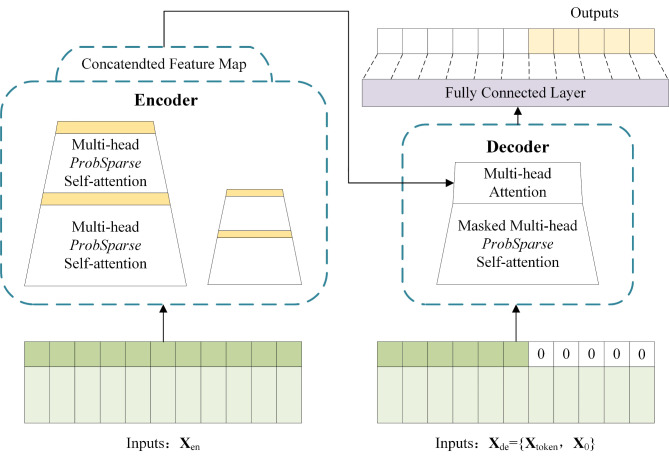
The Informer model is an enhanced model based on the Transformer suggested by Zhou, et al.⁴⁶, which has been extensively utilized in time series predicting tasks in finance, energy, transportation, and other fields⁴⁷. The model consists of three core modules: an embedding module, an encoder module, and a decoder module, which work together to enhance the accuracy of the forecast⁴⁸. The structure of Informer is schematically seen in Fig. 1. The following is the model implementation procedure⁴⁹:

Fig. 1.

Schematic structure of Informer.

The input of the Informer model includes the feature scalar , the location-encoded information PE, and the global timestamp SE with the following expression:

2

3

4

where i∈{1,…, L_x};j∈{1,…,}; L_x is the input sequence’s length; d_model is the feature dimension of the input; and is a factor that balances the size between the scalar mapping and the local/global embedding.

In the encoder module, the Informer innovates ProbSparse self-attention. This method efficiently identifies and focuses on dominant features in a sequence, significantly reducing computational time complexity and memory requirements while maintaining prediction accuracy⁵⁰.

Defining the standard for measuring sparsity: the KL divergence of attention probability and uniformly distributed . Determine whether q_i is sparse or uniform by calculating KL divergence.

5

Removing the constant, the sparsity metric may be described as:

6

The number of the dominant query is . The definition of ProbSparse self-attention is:

7

In addition, the encoder module employs the distillation operation of self-attention distilling. This technique drastically reduces the time dimension of the input sequences and further optimizes the model’s efficiency. The distillation process from layer j to layer j + 1 is as follows:

8

where Conv1d denotes a one-dimensional filter, ELU represents the activation function, and MaxPool represents the maximum pooling layer.

The decoder module, on the other hand, employs a generative decoding strategy, which allows the model to generate all predictions in a single step centrally, thus simplifying the prediction process and increasing efficiency⁵¹.

9

where denotes the input to the decoder module (decoding layer); denotes the known sequence before the target sequence; denotes the target sequence.

BiGRU

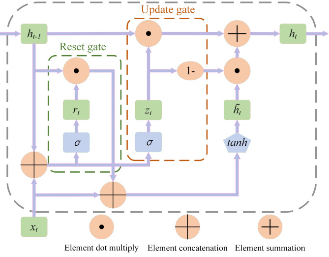
GRU is a neural network for predicting time series proposed by Chung, et al.⁵² and developed from recurrent neural network (RNN). The structure of the GRU unit is relatively simplified. GRU consists of two gates: a reset gate and an update gate. The reset gate controls how much past information contributes to the current update, and the update gate determines how much the current input affects the state of the update³⁸. Compared with other complex sequence processing models (such as LSTM), GRU has fewer parameters and faster training speed while maintaining the ability to deal with long-distance dependencies. The structure of GRU is seen in Fig. 2. Here is how GRU is specifically implemented:⁵³:

10

11

12

13

Fig. 2.

Schematic structure of the GRU.

where z_t, r_t are the update gate output and reset gate output at moment t, respectively; x_t is the input variable at moment t; h_t, h_t−1 are the hidden layer outputs at the current and previous moments, respectively; is the backfill hidden state vector at moment t; σ is the sigmoid activation function; W_z, W_r, W, U_z, U_r, U are the weight matrices.

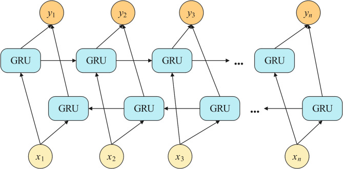
In time series analysis, the current state may be affected by both past and future states. The BiGRU model is an improved model that builds on the GRU, which consists of a forward GRU and an inverse GRU to capture information more comprehensively by processing data in both directions⁵⁴. This particular bi-directional structure allows the state at each point in time to take into account both previous and future information, enabling the model to predict and analyze the data more accurately, thus increasing the model’s comprehension of the data⁵⁵. Figure 3 illustrates the basic principle of the BiGRU model.

Fig. 3.

Schematic framework of BiGRU.

MHSA

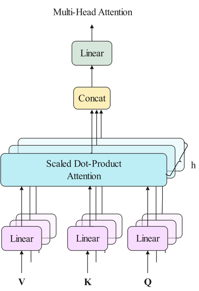
The MHSA is a crucial technique in deep learning, which maps inputs into different linear spaces by introducing multiple attention heads, computes attention independently within each space, and finally fuses the results of these attentions⁵⁶. This method elevates the model’s ability to represent complex features. When dealing with data containing noise or outliers, the MHSA can automatically adjust the weights to reduce the impacts of these negative factors and enhance the accuracy of the prediction and the diversity of the information processed⁵⁷. The following are the specific steps of the MHSA⁵⁸, and its general process is seen in Fig. 4.

Fig. 4.

Schematic diagram of the framework of the MHSA.

Assuming that the input weight matrix X=[x₁,x₂,…x_n], the query vector Q, the key vector K, and the value vector V are obtained by a cubic linear transformation which is implemented as follows:

14

where W_q, W_k, and W_v are weight matrices.

For every head, the attention calculation procedure yields a single feature. The computation process of its output is the following:

15

where d_k represents the dimension of the query vector in k.

Next, the output of each attention is spliced to obtain the final value, which is implemented as follows:

16

where W₀ is the output projection matrix, Concat denotes splicing, and head_i denotes the output of each head.

The proposed SMGformer model

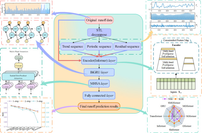
In this study, the SMGfomer runoff forecast model is developed, which learns the intrinsic features of runoff sequences by integrating multiple structures to get more precise forecast outcomes. First, the original runoff data are preprocessed by the STL decomposition method, which decomposes them into trend, period, and residual terms and constructs a multi-feature input set based on “sequence-sequence”, which integrates the original runoff sequences with their decomposed multi-feature sequences to provide a more comprehensive input dataset for the model. This step aims to reduce the nonlinear characteristics of the data so that the model more precisely captures the cyclical and trending nature of the runoff. The core structure of the predictive model building phase consists of three main components: the Informer’s Encoder layer, the BiGRU layer, and the MHSA layer. These components are connected serially to form a robust learning framework. The model first processes the input data through Informer’s Encoder layer, which is responsible for capturing and extracting critical features in the sequence. These features are then learned and extracted through the BiGRU layer to efficiently capture the sequence data’s temporal relationships, thereby enriching the model’s comprehension of variation in time series. Next, the output of the BiGRU layer is processed using the MHSA layer, which enhances the model’s emphasis on different parts of the sequence through parallel computation to realize the weight allocation among features. Finally, in the output layer stage, the fully connected layer transforms to get the MHSA layer’s output final monthly runoff projection. The overall structure of the model suggested by the model is seen in Fig. 5, and the specific steps are as follows:

Fig. 5.

Monthly runoff forecast model of the suggested SMGformer.

Step 1: Extract the raw runoff data’s trend, period, and residual terms using the STL decomposition.

Step 2: Combine the decomposed trend, period, and residual terms and the original runoff sequence into a multi-feature input set to provide a rich information source for the model.

Step 3: Use the Informer’s Encoder layer to perform feature extraction on the normalized multi-feature input set to capture the critical information in the sequence.

Step 4: The BiGRU layer is introduced to learn further and extract the features, capturing the temporal dependency of the sequence data through a two-way learning mechanism.

Step 5: The BiGRU layer’s output is processed using the MHSA layer to realize the weight allocation among features.

Step 6: Finally, the MHSA layer’s output is transformed into a forecast result through the Fully Connected Layer and reverse normalized to generate the final monthly runoff forecast value.

Case studies

Overview of the dataset

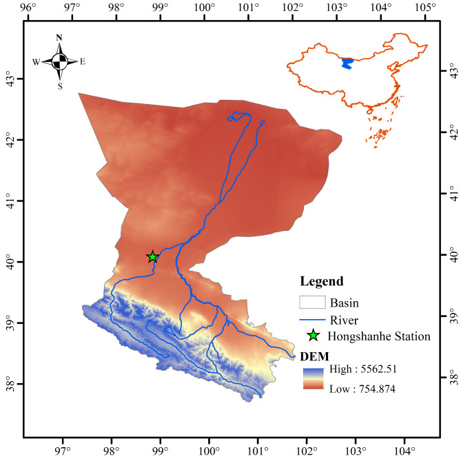
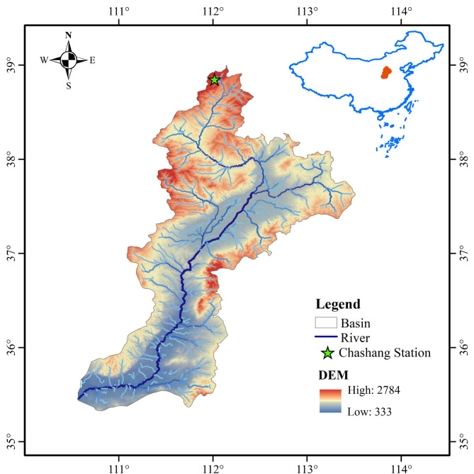
This study uses monthly runoff data from the Hongshanhe station in the Heihe River basin in Northwest China and the Chashang station in the Fen River basin in North China. The Heihe River basin is the second largest inland in northwest China, located in the central part of the Hexi Corridor. It is the largest inland river basin in the western part of Gansu and Mongolia, with a total length of 821 km and a basin area of about 142,900 km². Fen River Basin is the second largest tributary of the Yellow River Basin, located on the eastern edge of the Loess Plateau, with a total length of 716 km and a basin area of 39,741 km².

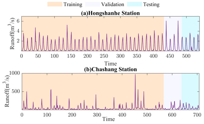
As shown in Table 1, there are significant differences in the maximum, minimum, average, center, and variance of runoff data between the two stations. This is because the northwest region of China usually has scarce rainfall, a dry climate, and high and complex terrain; The North China region has relatively more rainfall, mild climate, relatively flat terrain, and less variation. Considering the significant differences in rainfall, climate, elevation, and other aspects between the northwest and northern regions of China, Hongshanhe station and Chashang station are selected as case studies. Hongshanhe station and Chashang station are affected by the monsoon climate, with significant differences in precipitation and drastic changes in runoff. By studying the runoff patterns at Hongshanhe station and Chashang station, we can better understand the runoff characteristics under different geographical and climatic conditions, thereby verifying the applicability and robustness of the proposed model under different hydrological conditions, and providing reference value for water resource management and planning in different regions. This study selects the measured monthly runoff data from 1960 to 2004 at Hongshanhe station and 1958–2016 at Chashang station. The selected datasets are divided into training datasets, validation datasets, and test datasets, of which 80% are training datasets, 10% are validation datasets, and 10% are test datasets. The basic information of the dataset is shown in Table 1. The partitioning results of the dataset are shown in Table 2. A schematic diagram of the watersheds where the two stations are located is shown in Figs. 6 and 7. The measured monthly runoff sequence of the two stations is shown in Fig. 8.

Table 1.

Basic information about the monthly runoff dataset.

Site	Minimum(m3/s)	Maximum(m3/s)	Mean(m3/s)	Median (m3/s)	Variance (m3/s)
Hongshanhe	0.04	6.1	0.83	0.23	1.18
Chashang	5.0	972.0	47.6	24.0	5566.20

Table 2.

Dataset partitioning results.

Site	Time	Scale	Number of training sets	Number of validation sets	Number of test sets
Hongshanhe	1960–2004	Monthly	432	54	54
Chashang	1958–2016	Monthly	566	71	71

Fig. 6.

Schematic diagram of the Heihe River Basin.

Fig. 7.

Schematic diagram of the Fenhe River Basin.

Fig. 8.

Schematic diagram of the original sequence.

Experimental settings

To assess the effectiveness of SMGformer, eight models are selected to compare with it in this study, including LSTM, GRU, Transformer, Informer, SInformer, Gformer, SGformer, and MGformer models. LSTM, GRU, Transformer, and Informer, which are widely used as benchmark models, are used to measure the basic performance of SMGformer; SInfomer, Gformer, SGformer, and MGformer are used to evaluate the improvement effect of SMGformer on complex sequence modeling by combining STL decomposition, MHSA, and other strategies. These comparisons aim to reveal the superiority of SMGformer in predictive performance. Among them, the SInfomer, Gformer, SGformer, and MGformer models are shown in Table 3. The model input part Y_t stands for the original runoff sequence, T_t stands for the trend term, S_t stands for the period term, and R_t stands for the residual term.

Table 3.

Description of the experimental model.

Model	Input	Core structure
SInformer	(Tt, St, Rt, Yt)	Informer
Gformer	(Yt)	Encoder(Informer) + BiGRU
SGformer	(Tt, St, Rt, Yt)	Encoder(Informer) + BiGRU
MGformer	(Yt)	Encoder(Informer) + BiGRU + MHSA
SMGformer	(Tt, St, Rt, Yt)	Encoder(Informer) + BiGRU + MHSA

Due to the significant impact of the head_size in the Informer model on the forecast results, we select the head_size of 6, 8, and 10 for comparative experiments. Table 4 shows the predictive performance evaluation indicators of Informer for different head_sizes of two stations. The results indicate that when the head_size is 8, both experimental stations have the best predictive results. Therefore, set the head_size of the Informer to 8. Reference papers^47,59,60, set the batch_size of Informer to 32, Encoder_1ayers to 2, Decoder_1ayers to 1, and d_model to 512. Reference papers^61,62, set the hidden_size of LSTM and GRU to 265. To maintain consistency in experimental conditions, synchronize the corresponding parameters of other models. The other parameter settings for Informer and other models are shown in Table 5.

Table 4.

Results of predictive evaluation indicators for different head values.

Site	Head	MAE	RMSE	NSE	KGE
Hongshanhe	6	0.273	0.332	0.908	0.813
	8	0.204	0.277	0.936	0.915
	10	0.210	0.280	0.934	0.905
Chashang	6	22.082	32.487	0.486	0.708
	8	21.630	32.453	0.487	0.716
	10	22.481	32.915	0.473	0.702

Table 5.

Parameter settings of the models.

Model	Parameter settings
	Parameter	Value
STL	Period	12
LSTM	Hidden_layers	2
	Hidden_size	256
	Learning rate	0.001
	Epochs	100
	Optimizer	Adam
GRU	Hidden_layers Hidden_size Learning rate Epochs Optimizer	2 256 0.001 100 Adam
Transformer	Encoder	2
	Decoder	1
	Batch_size	32
	Early stopping	7
	Loss function	MSE
	Epochs	100
	Head_size	8
	d_model	512
Informer/ SInformer	Encoder	2
	Decoder Batch_size Early stopping Loss function Epochs	1 32 7 MSE 100
	Head_size	8
	d_model	512
Gformer/ SGformer	BiGRU_layers	2
	Hidden_size	256
	Encoder	2
	Batch_size	32
	Early stopping	7
	Loss function	MSE
	Epochs	100
	Head_size	8
	d_model	512
MGformer/ SMGformer	BiGRU_layers	2
	Hidden_size	256
	Encoder	2
	Batch_size Early stopping Loss function Epochs Head_size	32 7 MSE 100 8
	d_model	512
	MHSA_head_size	2

Evaluation metrics

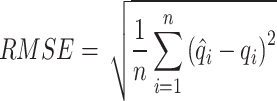
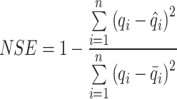
In this study, we utilized the following metrics measures to evaluate and analyze the models’ performance: mean absolute error (MAE), root-mean-square deviation (RMSE), Nash-Sutcliffe efficiency coefficient (NSE), and Kling-Gupta efficiency coefficient (KGE). MAE and RMSE assess the error magnitude between forecasted and actual values. The closer the MAE and RMSE values are to 0, the smaller the forecast error and the higher the forecast accuracy. NSE and KGE are used to measure the performance of hydrological forecast models. Generally speaking, the closer the values of NSE and KGE are to 1, the better the fitting effect of the model. The following defines these four metrics:

17

18

19

20

whereis the observed runoff,is the forecasted runoff;is the average of observed runoff; is the average of forecasted runoff;is variability bias;is the mean bias; R is the linear correlation coefficient; and represents the standard deviation and the mean, respectively.

Analysis of results

This section details the SMGformer model and the eight benchmark models’ forecast outcomes. The original runoff sequences are modeled using different methods based on the above description. To validate the reliability and accuracy of the suggested SMGformer integrated forecast model, this paper analyzes and discusses the forecast results from two perspectives: one-step and multi-step.

The model’s forecast procedure consists of three phases: training, validation, and testing. The training set is used to train the model, the validation set is used to tune the model’s hyperparameters, and the test set is used to evaluate the model’s performance. Therefore, the results of the test set are discussed in this paper.

Model input

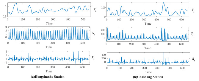
Due to the uncertainty and ambiguity of the runoff sequences, this study uses STL to decompose the runoff sequences to extract their intrinsic features. The STL decomposition decomposes the monthly runoff sequences of Hongshanhe and Chashang stations into trend, period, and residual terms, respectively, as shown in Fig. 9.

Fig. 9.

STL decomposition diagram.

Figure 9 shows that the trend, period, and residual terms of the monthly runoff series extracted from the STL decomposition possess different complexities. The trend series reveals its long-term evolution direction, which is manifested by the increase or decrease of runoff volume; the period series reflects the repetitive pattern over some time, and this regular fluctuation helps the model to deeply understand the characteristics of runoff within a specific period; the residual series represents the randomly changing part of the runoff series, and its fluctuation is directly related to the precision of the overall runoff forecast. Together, these three features constitute the complex dynamic of the monthly runoff sequence, reflecting its multidimensional characteristics.

One-step prediction results

To confirm the suggested SMGformer model’s efficacy in runoff forecasting, this paper compares the SMGformer model with eight benchmark models (LSTM, GRU, Transformer, Informer, SInformer, Gformer, SGformer, MGformer), and the outcomes of the evaluation indexes are seen in Table 6.

Table 6.

Results of evaluation metrics for the models.

Site	Model	MAE	RMSE	NSE	KGE
Hongshanhe	SMGformer	0.118	0.172	0.975	0.978
	MGformer	0.134	0.200	0.967	0.970
	SGformer	0.148	0.211	0.963	0.950
	Gformer	0.168	0.244	0.951	0.943
	SInformer	0.191	0.259	0.945	0.925
	Informer	0.204	0.277	0.936	0.915
	Transformer	0.224	0.319	0.916	0.912
	GRU	0.219	0.307	0.921	0.909
	LSTM	0.217	0.316	0.917	0.880
Chashang	SMGformer	13.714	18.307	0.837	0.908
	MGformer	20.664	28.202	0.613	0.762
	SGformer	17.014	23.926	0.721	0.773
	Gformer	21.283	29.545	0.575	0.729
	SInformer	20.836	29.645	0.572	0.747
	Informer	21.630	32.453	0.487	0.716
	Transformer	23.537	34.589	0.418	0.638
	GRU	22.713	33.509	0.453	0.679
	LSTM	22.384	34.345	0.426	0.637

Analyzing Table 6, the following conclusions can be obtained:

(1) Informer has relatively high accuracy compared to Transformer, GRU, and LSTM. For Hongshanhe and Chashang stations, in comparison to Transformer, GRU, and LSTM, the Informer has the biggest NSE and KGE, the smallest MAE, and the RMSE. To further improve the quality of the model, this paper improves Informer. By integrating the Informer’s Encoder layer and BiGRU, the Gformer model is obtained, and the Gformer is made better to capture the long-term dependence in time sequence data. For Hongshanhe station, the NSE and KGE of Gformer are as high as 0.951 and 0.943, respectively. Compared with Informer, the MAE decreases by 17.6%, and the RMSE decreases by 11.9%. For Chashang station, the MAE and RMSE of Gformer decreased by 1.6% and 8.9%, respectively, compared to Informer; both NSE and KGE improved significantly. This improvement indicates that Informer’s Encoder layer effectively extracts global features in the runoff sequences, while BiGRU captures local dependencies in the runoff sequences through its bidirectional loop structure. This combination realizes the effective fusion of global and local features, enabling the Gformer model to comprehensively understand the intrinsic structure and dynamic changes of time series data. The MGformer model is obtained by adding MHSA to Gformer, which improves the model’s power to handle complex sequence features. At Hongshanhe, compared with Gformer, MGformer reduces 20.2% in MAE and 18.0% in RMSE and increases NSE from 0.951 to 0.967 KGE from 0.943 to 0.970. For the Chashang station, compared with Gformer, MGformer reduces the MAE and RMSE, respectively, by 2.9% and 4.5%. There is an improvement of 9.7% on NSE and 4.5% on KGE. The above results indicate that further introducing the MHSA based on Gformer can effectively enhance the predictive precision of the model.

(2) To improve the quality of model input data, this paper adopts the STL decomposition technique to pre-process the runoff sequences to extract the deep intrinsic features of the runoff sequences and constructs a multi-feature set containing the trend, the period, the residuals, and the original runoff sequences, to realize the model input of the “sequence-sequence” method. The results show that the prediction accuracies of SInformer, SGformer, and SMGformer models based on multi-feature inputs significantly outperform those of Informer, Gformer, and MGformer models, which only rely on the input of raw runoff sequences. At Hongshanhe station, the NSE and KGE of SGMformer were as high as 0.975 and 0.978, respectively, and the MAE and RMSE were reduced by 11.9% and 14.0%, respectively, compared with MGformer. Compared to Gformer, SGformer has 1.3% and 0.7% higher NSE and KGE and 11.9% and 13.5% lower MAE and RMSE, respectively. Compared to Informer, SInformer had a 6.3% and 6.5% decrease in MAE and RMSE, respectively, and an increase in NSE and KGE. For Chashang station, the MAE and RMSE of SMGformer are 33.6% and 35.1% lower than MGformer; NSE increases from 0.631 to 0.837; and KGE increases from 0.762 to 0.908. Compared to Gformer, the MAE and RMSE of SGformer decreased by 20.1% and 19.0%, respectively, and both NSE and KGE improved significantly. Compared with Informer, SInformer’s MAE and RMSE decreased by 3.7% and 8.7%, while NSE and KGE enhanced by 17.5% and 4.3%, respectively. Thus, the STL decomposition technique and the SInformer, SGformer, and SMGformer models based on the “sequence-sequence” inputs can significantly enhance the precision of runoff forecasting, which thoroughly verifies the efficiency of the STL decomposition technique and the multi-feature inputs.

To visualize the research results in Table 6 and to compare the different models’ performance in runoff forecasting, bar charts, radar charts, line graphs, scatter plots, and Taylor diagrams are used to show the differences in the performance of each model.

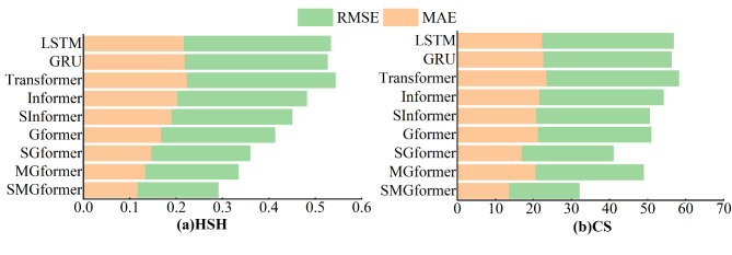
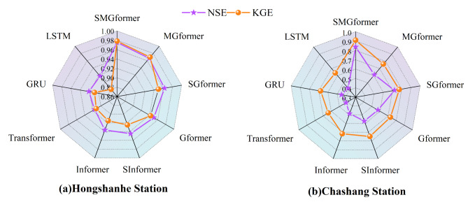
Figure 10 displays the RMSE and MAE metrics of each model in the form of bar charts, and it is evident that the SMGformer model has the smallest RMSE and MAE values. Figure 11 presents each model’s NSE and KGE metrics in the form of a radar chart, where the center of the radar chart represents the starting point and multiple axes radiate outward from the center. Each axis corresponds to a model, and specific symbols are used to label each model’s NSE and KGE values. The closer these symbols are to the boundary of the radar plot, the closer the NSE and KGE values converge to 1, meaning that the model predictions are closer to the actual observations. It can be observed in the figure that the symbols representing the SMGformer model are located near the boundary, indicating that its prediction ability is extremely excellent. This result proves that the model suggested in this research significantly reduces the abnormal fluctuations in the forecast outcomes.

Fig. 10.

Results of evaluation metrics for MAE and RMSE.

Fig. 11.

Radar plot of NSE and KGE results.

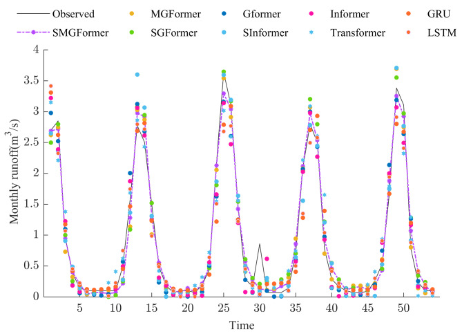
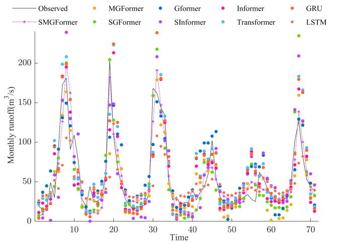
Figures 12 and 13 show the predicted values of the eight models for the Hongshanhe and Chashang stations. It is clear from the figures that the statistical dispersion between predicted and measured values of the LSTM, GRU, and Transformer is relatively high compared to other models. The trend line of the improved Gformer and MGformer predicted values is close to the fluctuation trend of the measured values by and by. Compared with the Informer, Gformer, and MGformer models, the SInformer, SGformer, and SMGformer model effectively improves the fit of the series. Among them, forecast and observed values’ trend lines are the same. This indicates that the SMGformer model is more accurate in capturing variations in the runoff sequence and dramatically improves the model’s predictive ability.

Fig. 12.

Forecast results of various models at Hongshanhe station.

Fig. 13.

Forecast results of various models at Chashang station.

Figures S1and S2 in the supplementary materials display the scatter density plots of measured and forecasted flows for different prediction models, where R² is the coefficient of determination, which indicates the proportion of changes in the dependent variable y that can be explained by independent variable x. It can be observed that the SMGformer model has the highest predicted and measured fit, close to 1. This result confirms the reliability of the suggested model.

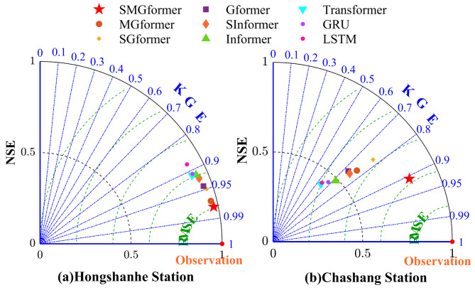
Figures 14 presents the Taylor plots of the predicted results for each model testing stage. The horizontal and vertical axes in the Taylor plot represent NSE, the radial lines represent KGE, the dashed lines represent RMSE, and the symbols represent each model. When NSE is closer to 1, the azimuth of the model icon is smaller and the RMSE radius is smaller. The closer the model icon is to the observation point, the closer the forecasted results of the model are to real values. From the figure, it can be seen that the SMGformer model has the best forecast results.

Fig. 14.

Taylor plots of evaluation indicators for each model.

In summary, this research reveals the positive impacts of model structure improvement and model inputs on runoff forecast accuracy by comparing and analyzing the above nine models. Gformer achieves the synergistic capture of global and local features by combining Informer’s Encoder layer with BiGRU. MGformer further enhances the processing of complex sequence features by introducing the mechanism of multiple attention capability. In addition, the combination of the STL decomposition technique and multi-feature input strategy significantly improves the model’s forecasting performance. These results validate the importance of model structure improvement and input data preprocessing and provide effective strategies and methods for runoff sequence forecasting.

Multi-step forecast results

To verify the suggested SMGformer model’s advantage in multi-step forecasting, this paper compares the SMGformer model with the above models. Table 7 lists the specific evaluation metrics of different models in months 1, 2, and 3.

Table 7.

Multi-step forecast results for each model.

Site	Model	1-step				2-step				3-step
		MAE	RMSE	NSE	KGE	MAE	RMSE	NSEC	KGE	MAE	RMSE	NSE	KGE
Hongshanhe	SMGformer	0.118	0.172	0.975	0.978	0.122	0.180	0.973	0.971	0.128	0.202	0.967	0.960
	MGformer	0.134	0.200	0.967	0.970	0.156	0.213	0.963	0.961	0.165	0.229	0.957	0.950
	SGformer	0.148	0.211	0.963	0.950	0.179	0.227	0.958	0.948	0.185	0.253	0.948	0.934
	Gformer	0.168	0.244	0.951	0.943	0.191	0.253	0.947	0.921	0.214	0.297	0.928	0.918
	SInformer	0.191	0.259	0.945	0.925	0.212	0.255	0.946	0.922	0.215	0.282	0.935	0.916
	Informer	0.204	0.277	0.936	0.915	0.237	0.297	0.928	0.912	0.253	0.314	0.920	0.900
	Transformer	0.224	0.319	0.916	0.912	0.256	0.336	0.906	0.846	0.321	0.496	0.796	0.874
	GRU	0.219	0.307	0.921	0.909	0.244	0.309	0.921	0.889	0.276	0.352	0.897	0.886
	LSTM	0.217	0.316	0.917	0.880	0.248	0.318	0.913	0.878	0.278	0.392	0.862	0.874
Chashang	SMGformer	13.714	18.307	0.837	0.908	14.701	20.690	0.794	0.845	15.346	22.704	0.755	0.805
	MGformer	20.664	28.202	0.613	0.762	22.358	31.581	0.520	0.726	23.880	34.075	0.449	0.676
	SGformer	17.014	23.926	0.721	0.773	20.717	24.153	0.719	0.761	21.733	26.089	0.677	0.741
	Gformer	21.283	29.545	0.575	0.729	23.211	32.117	0.504	0.684	25.929	36.053	0.383	0.630
	SInformer	20.836	29.645	0.572	0.747	23.969	30.358	0.557	0.711	24.406	32.006	0.514	0.597
	Informer	21.630	32.453	0.487	0.716	25.220	33.698	0.454	0.656	27.745	37.234	0.342	0.563
	Transformer	23.537	34.589	0.418	0.638	26.012	36.030	0.366	0.364	29.581	38.394	0.280	0.221
	GRU	22.713	33.509	0.453	0.679	25.700	34.695	0.412	0.393	28.009	38.091	0.291	0.278
	LSTM	22.384	34.345	0.426	0.637	25.861	35.300	0.397	0.363	29.142	38.312	0.287	0.257

From the forecast results in Table 7, it is evident that as the time step increases, the models’ forecast errors progressively rise, and the increasing trend is different for each model. At Hongshanhe and Chashang stations, compared to the other eight models, the SMGformer has the smallest MAE and RMSE and the largest NSE and KGE at step lengths of 2 and 3. Compared with Transformer, GRU, and LSTM, the Informer has a flatter decreasing accuracy trend at step lengths 2 and 3, which indicates that Informer performs better in long series forecast. At the 2th step, the SMGformer model’s MAE and RMSE decrease by 21.8% and 15.5%, respectively, and the NSE and KGE improve by 1.0% and 1.0%, respectively, in contrast to MGformer at the Hongshanhe station. Compared with SInformer, the SMGformer model’s RMSE and MAE are 29.4% and 42.5% lower, respectively, the NSE increases from 0.946 to 0.973, and the KGE increases from 0.922 to 0.971, respectively. At Chashang station, in contrast to the MGformer model, the MAE and RMSE of the SMGformer decreased by 34.2% and 34.5%, and NSE and KGE improved by 52.7% and 16.4%, respectively. The MAE and RMSE of the SMGformer model decreased by 38.7% and 31.8% compared to the SInformer model; the NSE increased from 0.557 to 0.794, and the KGE increased from 0.711 to 0.845. At the 3th step, at the Hongshanhe station, the SMGformer model demonstrates significant improvements over both SInformer and MGformer. Compared to SInformer, the SMGformer’s MAE and RMSE have decreased by 40.5% and 28.4%, respectively, while the NSE and KGE have improved by 3.4% and 4.8%. In contrast to MGformer, the SMGformer’s MAE and RMSE have decreased by 22.4% and 11.8%, with the NSE rising from 0.957 to 0.967, and the KGE increasing from 0.95 to 0.96. At Chashang station, compared with the SInformer model, the SMGformer’s MAE and RMSE are decreased by 37.1% and 29.1%, and NSE and KGE are enhanced by 46.7% and 34.8%, respectively. Compared to MGformer, the SMGformer’s MAE and RMSE are decreased by 35.7% and 33.4%, respectively, and the NSE is improved from 0.449 to 0.755, and the KGE is improved from 0.676 to 0.805. These results indicate that the model improvement and the multi-feature input strategy increase the effective foresight period of the forecast.

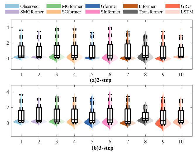
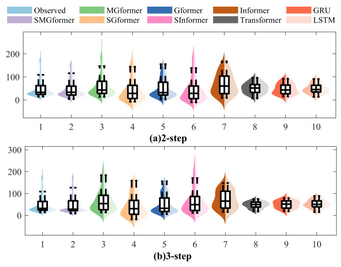
Figures 15 and 16 show the violin plots of the forecasted and observed values of the nine models at two stations at steps 2th and 3th, which clearly show that the kernel density curves of the measured runoff sequences are characterized by multiple peaks with flat and broad peak shapes, concentrated data and large deviation values, which indicate that the measured sequences have intense volatility. Meanwhile, the SMGformer model proposed in this study has a kernel density plot trend that agrees with the observed data, which indicates that the model has a better forecast performance and proves the effectiveness of the SMGformer model in improving the effective foresight period of the model.

Fig. 15.

Violin plot of multi-step forecast results for the Hongshanhe station.

Fig. 16.

Violin plots of multi-step forecast results for the Chashang station.

Figures S3 and S4 in the supplementary materials show the two metrics, NSE and RMSE, respectively. It is evident that the evaluation performance of each model decreases from 1th step to 3th step, but the decrease of the SMGformer model is more moderate, which shows that in the 3th step, our proposed SMGformer model still has good data fitting ability. SMGformer has the smallest overall forecast error and the slightest decrease in accuracy as the prediction point moves back. Among them, the Transformer significantly decreases in the third step forecast process, which may be due to the high computational complexity and memory consumption of the Transformer model caused by its self-attention mechanism secondary calculation when processing long sequences, which may limit the model’s multi-step forecast ability⁶³. In addition, the dynamic decoding process of the Transformer results in slow inference speed when inferring long sequence outputs, which may also affect multi-step forecast accuracy⁶⁴.

Discussion

Improvement of the model input end

To further validate the effectiveness of the “sequence sequence” multi-feature input based on STL decomposition, we explain it from two perspectives: computational complexity and prediction accuracy. Taking single-step forecast as an example, an item-by-item sequence forecast model (STL-MGformer, STL-Informer) is constructed to test the effectiveness of the multi-feature sequence prediction model (SMGformer, SInformer) in improving the input end. Item-by-item sequence forecast is achieved by separately forecasting the trend sequence, periodic sequence, and residual sequence obtained from STL decomposition, and then superimposing the forecast results of each sequence to obtain the final prediction result. Table 8 shows the predictive evaluation indicators of the model, and Table 9 shows the running time of the model.

Table 8.

Results of predictive evaluation indicators for the model.

Site	Model	MAE	RMSE	NSE	KGE
Hongshanhe	STL-MGformer	0.127	0.181	0.969	0.972
	STL-Informer	0.201	0.274	0.938	0.917
Chashang	STL-MGformer	16.370	24.175	0.743	0.813
	STL-Informer	21.256	30.800	0.538	0.724

Table 9.

Running time of the model.

Site	Model	Run time(s)
Hongshanhe	SMGformer	11.53
	SInformer	13.82
	STL-MGformer	32.87
	STL-Informer	34.75
Chashang	SMGformer	18.18
	SInformer	14.12
	STL-MGformer	39.69
	STL-Informer	35.46

By comparing the performance of SMGformer and SInformer in Table 6 with the item-by-item sequence forecast models STL-MGformer and STL-Informer in Table 8 at two sites, respectively. It can be observed that compared to the STL-MGformer model, SMGformer has reduced MAE and RMSE at both stations, while NSE and KGE have improved. Similarly, compared to the STL-Informer model, SInformer showed improved performance at both sites. In addition, from Table 9, it can be seen that compared to the sequential forecast model, SMGformer and SInfomer have reduced their running time at Hongshanhe station by 64.9% and 60.3%, respectively, and at the Chashang station by 54.2% and 60.2%, respectively. These results demonstrate that compared to decomposing and forecasting item-by-item before stacking, the multi-feature input approach is more efficient for feature extraction of complex time series while improving prediction accuracy.

In summary, the “sequence-sequence” multi-feature input method based on STL decomposition significantly improves the prediction accuracy of the model and greatly reduces computational complexity by effectively integrating different feature information. These results indicate that using a “sequence-sequence” based multi-feature input method can better integrate information from different features, capture the multidimensional characteristics of data, and enable SMGformer to predict complex time series data more efficiently and accurately.

Improvement of the model structure end

In the model structure of this study, we propose a new model structure MGformer to enhance the accuracy of runoff sequence forecast. The traditional Informer model is mainly based on one-way information flow, using only past data to predict future data, which means that it only considers information from past time points during the encoding stage. To overcome this limitation, we concatenate the Informer’s Encoder layer with the BiGRU model, enabling the model to simultaneously capture the before and after dependencies in the sequence. In addition, to further emphasize the influence of key information, we use MHSA to optimize the output of BiGRU, thereby achieving more accurate forecasts.

By concatenating the Informer’s Encoder layer, BiGRU layer, and MHSA layer, the MGformer model significantly improves the accuracy of forecast. To verify the effectiveness of the MGformer model’s structural improvement, taking single-step forecast as an example, we design two new hybrid models: The Informer-Transformer model and the Transformer-Informer model. Specifically, the Informer-Transformer model concatenates the Informer model with the Transformer model, while the Transformer-Informer model concatenates the Transformer model with the Informer model. The forecasted results of the model are shown in Table 10.

Table 10.

Prediction and evaluation index results of the hybrid model.

Site	Model	MAE	RMSE	NSE	KGE
Hongshanhe	Informer-Transformer	0.221	0.324	0.913	0.896
	Transformer-Informer	0.211	0.289	0.928	0.921
Chashang	Informer-Transformer	22.846	33.322	0.459	0.713
	Transformer-Informer	23.719	34.766	0.413	0.685

From Table 10, it can be seen that compared with the hybrid models Informer-Transformer and Transformer-Informer, the MGformer model has multiple advantages. Firstly, MGformer combines the feature extraction capability of the Informer’s Encoder layer, the pre - and post-dependency capture capability of the BiGRU layer, and the key information attention of the MHSA. This design is more effective in capturing complex data features. The experimental results also confirmed the superiority of this structure. For example, at Hongshanhe station, the MAE and RMSE of MGformer are 0.134 and 0.200, respectively, significantly better than Informer-Transformer (0.221 and 0.324) and Transformer-Informer (0.211 and 0.289). At Chashang station, the MAE and RMSE of MGformer are 20.664 and 28.202, respectively, which are also better than Informer-Transformer (22.846 and 33.322) and Transformer-Informer (23.719 and 34.766). The NSE and KGE of the MGformer models in the two experimental stations are also higher than those of the mixed model. These results indicate that although hybrid models can also capture more information, MGformer achieves higher prediction accuracy by designing a hierarchical structure that allows each component in the model to leverage its strengths.

In summary, compared to hybrid models, the MGformer model improves the internal structure of the model and fully utilizes the advantages of the Informer’s Encoder layer, BiGRU, and MHSA to achieve more accurate predictions.

Conclusion

This paper proposes a new model for monthly runoff forecasting called SMGformer. The model first uses STL to extract the raw runoff sequence’s trend, period, and residual features. Then, these features are combined with the raw runoff sequence to create a multi-feature input set. Next, the critical information of this feature set is captured using the Informer’s Encoder layer. Subsequently, the temporal dependence of the sequence data is captured through the bidirectional learning mechanism of the BiGRU layer, and the output of the BiGRU layer is optimized using the MHSA layer. Finally, the output of the MHSA layer is transformed into the final forecast result through the fully connected layer. The following conclusions are drawn in this paper:

(1) The STL decomposition technique is used to analyze the runoff sequence, aiming at reducing the non-stationarity of the runoff series and extracting the trend, period, and residual features of the runoff sequence to construct a multi-feature input set based on the intrinsic features of the runoff sequence. This input method enhances the model’s potential to mine the inherent characteristics of runoff and more accurately captures the evolutionary characteristics of the runoff sequence, thereby providing strong technical support for runoff forecast and analysis.

(2) A proposed MGformer forecast model integrates three critical layers in tandem: the Informer’s Encoder layer, the BiGRU layer, and the MHSA layer. In this way, the advantages of each critical layer are integrated, the learning ability of the intrinsic characteristics of runoff is emphasized, the utilization rate of the model on runoff time-series characteristics is enhanced, the limitations of a single model in predicting strongly fluctuating runoff sequences are reduced, and the effective foresight period of the model is prolonged, to realize the efficient forecasting capability of the model.

(3) To verify the model’s capacity for generalization, data sets from two experimental stations are applied for experimental validation. The outcomes demonstrate the SMGformer’s superior performance. At the Hongshanhe station, the mean MAE of the 1th, 2th, and 3th steps is 0.12, and the mean RMSE is 0.18, which are significantly lower than the error outcomes of the comparison model, and the NSE and KGE of step 3 are as high as 0.967 and 0.960, respectively. At the Chashang station, compared with the Informer deep learning model, the MAE and RMSE forecast results of the 1th, 2th, and 3th steps are reduced by 36.6% and 43.6%, 41.7% and 38.6%, and 44.7% and 39.0%, respectively. This outcome shows that the suggested SMGformer model can extend the effective foresight period of runoff forecasting.

(4) Although the proposed new SMGformer model provides a new perspective for runoff forecasting and related fields, there are still some limitations that need to be addressed in future research. For example, this study does not consider the impact of factors such as rainfall and evaporation on runoff forecast. In addition, the model is only validated based on data from two experimental stations, and future research should include more experimental stations under different geographical and climatic conditions to ensure the robustness and generality of the model. Finally, this study only applies the model to monthly runoff forecasting, and future research should attempt to extend it to handle different time scales, such as daily or seasonal forecasting. These improvements will help further extend the effective forecast period of runoff forecasting.

Electronic supplementary material

Below is the link to the electronic supplementary material.(Supplementary material 1 already includes 4 attached images. It is recommended to either retain only supplementary material 1 or attach one image each to supplementary materials 1, 2, 3, and 4 respectively.)

Author contributions

Wen-chuan Wang: Conceptualization, Methodology, Investigation, Writing – original draft, Formal analysis. Miao Gu：Writing – original draft, Methodology, Data curation. Yang-hao Hong: Methodology, Writing –original draft. Xiao-xue Hu: Writing – original draft, Formal analysis. Hong-fei Zang: Writing – original draft, Investigation. Xiao-nan Chen: Writing – original draft. Yan-guo Jin: Writing – original draft.

Data availability

The data are available from the corresponding author on reasonable request.

Declarations

Competing interests

The authors declare no competing interests.

References

- 1.Amini, A., Dolatshahi, M. & Kerachian, R. Real-time rainfall and runoff prediction by integrating BC-MODWT and automatically-tuned DNNs: comparing different deep learning models. J. Hydrol. 10.1016/j.jhydrol.2024.130804 (2024).
- 2.Zhao, H. et al. Long-term inflow forecast using meteorological data based on long short-term memory neural networks. J. Hydroinform 10.2166/hydro.2024.196 (2024).
- 3.Xu, D., Li, Z. & Wang, W. -c. An ensemble model for monthly runoff prediction using least squares support vector machine based on variational modal decomposition with dung beetle optimization algorithm and error correction strategy. J. Hydrol. 629, 130558. 10.1016/j.jhydrol.2023.130558 (2024). [Google Scholar]
- 4.Yuan, X., Chen, C., Lei, X. & Yuan, Y. Muhammad Adnan, R. Monthly runoff forecasting based on LSTM–ALO model. Stoch. Env. Res. Risk Assess. 32, 2199–2212. 10.1007/s00477-018-1560-y (2018). [Google Scholar]
- 5.Yan, L. et al. Climate-informed monthly runoff prediction model using machine learning and feature importance analysis. Front. Environ. Sci. 10.3389/fenvs.2022.1049840 (2022).
- 6.Bian, L., Qin, X., Zhang, C., Guo, P. & Wu, H. Application, interpretability and prediction of machine learning method combined with LSTM and LightGBM-a case study for runoff simulation in an arid area. J. Hydrol. 625, 130091. 10.1016/j.jhydrol.2023.130091 (2023). [Google Scholar]
- 7.Xie, Y. et al. Stacking ensemble learning models for daily runoff prediction using 1D and 2D CNNs. Expert Syst. Appl. 10.1016/j.eswa.2022.119469 (2023).
- 8.Yoon, H., Jun, S. C., Hyun, Y., Bae, G. O. & Lee, K. K. A comparative study of artificial neural networks and support vector machines for predicting groundwater levels in a coastal aquifer. J. Hydrol. 396, 128–138 (2011). [Google Scholar]
- 9.Mostafa, R. R., Kisi, O., Adnan, R. M., Sadeghifar, T. & Kuriqi, A. Modeling potential evapotranspiration by Improved Machine Learning methods using Limited Climatic Data. Water 15 (2023).
- 10.Adnan, R. M. et al. Pan evaporation estimation by relevance vector machine tuned with new metaheuristic algorithms using limited climatic data. Eng. Appl. Comput. Fluid Mech. 10.1080/19942060.2023.2192258 (2023).
- 11.Yue, Z., Ai, P., Xiong, C., Hong, M. & Song, Y. Mid- to long-term runoff prediction by combining the deep belief network and partial least-squares regression. J. Hydroinform. 22, 1283–1305. 10.2166/hydro.2020.022 (2020). [Google Scholar]
- 12.Adnan, R. M. et al. Estimating reference evapotranspiration using hybrid adaptive fuzzy inferencing coupled with heuristic algorithms. Comput. Electron. Agric. 10.1016/j.compag.2021.106541 (2021).
- 13.Adnan, R. M. et al. Modeling Multistep ahead dissolved Oxygen Concentration using Improved Support Vector machines by a hybrid metaheuristic algorithm. Sustainability 14 (2022).
- 14.Samantaray, S., Sawan Das, S. & Sahoo, A. Prakash Satapathy, D. Monthly runoff prediction at Baitarani river basin by support vector machine based on salp swarm algorithm. Ain Shams Eng. J. 13, 101732. 10.1016/j.asej.2022.101732 (2022). [Google Scholar]
- 15.Adnan, R. M. et al. Modelling groundwater level fluctuations by ELM merged advanced metaheuristic algorithms using hydroclimatic data. Geocarto Int. 38, 2158951. 10.1080/10106049.2022.2158951 (2023). [Google Scholar]
- 16.Hinton, G. E., Osindero, S. & Teh, Y. W. A fast learning algorithm for deep belief nets. Neural Comput. 18, 1527–1554. 10.1162/neco.2006.18.7.1527 (2006). [DOI] [PubMed] [Google Scholar]
- 17.Bai, S., Kolter, J. Z. & Koltun, V. An empirical evaluation of generic convolutional and recurrent networks for sequence modeling. ArXiv (2018).
- 18.Vaswani, A. et al. Attention is all you need. Neural Inform. Process. Syst. 10.48550/arXiv.1706.03762 (2017). [Google Scholar]
- 19.Guo, J. et al. Study on optimization and combination strategy of multiple daily runoff prediction models coupled with physical mechanism and LSTM. J. Hydrol. 10.1016/j.jhydrol.2023.129969 (2023).
- 20.Qiao, X. et al. Metaheuristic evolutionary deep learning model based on temporal convolutional network, improved aquila optimizer and random forest for rainfall-runoff simulation and multi-step runoff prediction. Expert Syst. Appl. 229, 120616. 10.1016/j.eswa.2023.120616 (2023). [Google Scholar]
- 21.Wei, X., Wang, G., Schmalz, B., Hagan, D. F. T. & Duan, Z. Evaluation of Transformer model and self-attention mechanism in the Yangtze River basin runoff prediction. J. Hydrol. 47, 101438. 10.1016/j.ejrh.2023.101438 (2023). [Google Scholar]
- 22.Yin, H. et al. Runoff predictions in new-gauged basins using two transformer-based models. J. Hydrol. 10.1016/j.jhydrol.2023.129684 (2023).
- 23.Ikram, R. M. et al. Water temperature prediction using improved deep learning methods through reptile search algorithm and weighted mean of vectors optimizer. J. Mar. Sci. Eng. 11 (2023).
- 24.Hu, F. et al. Incorporating multiple grid-based data in CNN-LSTM hybrid model for daily runoff prediction in the source region of the Yellow River Basin. J. Hydrolo 51, 101652. 10.1016/j.ejrh.2023.101652 (2024). [Google Scholar]
- 25.Li, W. et al. Application of a hybrid algorithm of LSTM and Transformer based on random search optimization for improving rainfall-runoff simulation. Sci. Rep. 14, 11184. 10.1038/s41598-024-62127-7 (2024). [DOI] [PMC free article] [PubMed] [Google Scholar]
- 26.Jia, C. et al. A performance degradation prediction model for PEMFC based on bi-directional long short-term memory and multi-head self-attention mechanism. Int. J. Hydrog. Energy 60, 133–146. 10.1016/j.ijhydene.2024.02.181 (2024). [Google Scholar]
- 27.Tu, B., Bai, K., Zhan, C. & Zhang, W. Real-time prediction of ROP based on GRU-Informer. Sci. Rep. 1410.1038/s41598-024-52261-7 (2024). [DOI] [PMC free article] [PubMed]
- 28.Gao, S. et al. A new seq2seq architecture for hourly runoff prediction using historical rainfall and runoff as input. J. Hydrol. 10.1016/j.jhydrol.2022.128099 (2022).
- 29.Ren, S., Wang, X., Zhou, X. & Zhou, Y. A novel hybrid model for stock price forecasting integrating Encoder Forest and Informer. Expert Syst. Appl. 234, 121080. 10.1016/j.eswa.2023.121080 (2023). [Google Scholar]
- 30.Ribalta Gené, M. et al. Sewer sediment deposition prediction using a two-stage machine learning solution. J. Hydroinform. 26, 727–743. 10.2166/hydro.2024.144 (2024). [Google Scholar]
- 31.Shi, Z. et al. WGformer: a Weibull-Gaussian Informer based model for wind speed prediction. Eng. Appl. Artif. Intell. 10.1016/j.engappai.2024.107891 (2024).
- 32.Fang, M. et al. The influence of optimization algorithm on the signal prediction accuracy of VMD-LSTM for the pumped storage hydropower unit. J. Energy Storage 78, 110187. 10.1016/j.est.2023.110187 (2024). [Google Scholar]
- 33.Liang, B. X., Hu, J. P., Liu, C. & Hong, B. Data pre-processing and artificial neural networks for tidal level prediction at the Pearl River Estuary. J. Hydroinform. 23, 368–382. 10.2166/hydro.2020.055 (2020). [Google Scholar]
- 34.Zeng, T. et al. A hybrid optimization prediction model for PM2.5 based on VMD and deep learning. Atmosp. Pollut. Res. 10.1016/j.apr.2024.102152 (2024).
- 35.Zhang, B., Song, C., Jiang, X. & Li, Y. Electricity price forecast based on the STL-TCN-NBEATS model. Heliyon 9, e13029. 10.1016/j.heliyon.2023.e13029 (2023). [DOI] [PMC free article] [PubMed]
- 36.Qi, X., Hong, C., Ye, T., Gu, L. & Wu, W. Frequency reconstruction oriented EMD-LSTM-AM based surface temperature prediction for lithium-ion battery. J. Energy Storage 84, 111001. 10.1016/j.est.2024.111001 (2024). [Google Scholar]
- 37.Zhang, X., Liu, F., Yin, Q., Qi, Y. & Sun, S. A runoff prediction method based on hyperparameter optimisation of a kernel extreme learning machine with multi-step decomposition. Sci. Rep. 13, 19341. 10.1038/s41598-023-46682-z (2023). [DOI] [PMC free article] [PubMed] [Google Scholar]
- 38.Chen, H., Wu, H., Kan, T., Zhang, J. & Li, H. Low-carbon economic dispatch of integrated energy system containing electric hydrogen production based on VMD-GRU short-term wind power prediction. Int. J. Electr. Power Energy Syst. 154, 109420. 10.1016/j.ijepes.2023.109420 (2023). [Google Scholar]
- 39.Fang, J. et al. Ensemble learning using multivariate variational mode decomposition based on the transformer for multi-step-ahead streamflow forecasting. J. Hydrol. 10.1016/j.jhydrol.2024.131275 (2024).
- 40.Qin, L., Li, W. & Li, S. Effective passenger flow forecasting using STL and ESN based on two improvement strategies. Neurocomputing 356, 244–256. 10.1016/j.neucom.2019.04.061 (2019). [Google Scholar]
- 41.Wu, Y. et al. Effective LSTMs with seasonal-trend decomposition and adaptive learning and niching-based backtracking search algorithm for time series forecasting. Expert Syst. Appl. 10.1016/j.eswa.2023.121202 (2024).
- 42.Xu, Z., Mo, L., Zhou, J., Fang, W. & Qin, H. Stepwise decomposition-integration-prediction framework for runoff forecasting considering boundary correction. Sci. Total Environ. 851, 158342. 10.1016/j.scitotenv.2022.158342 (2022). [DOI] [PubMed] [Google Scholar]
- 43.Cleveland, R. B. & Cleveland, W. S. STL: a seasonal-trend decomposition procedure based on Loess. J. Official Stat. 6, 1–7. 10.1109/IJCNN52387.2021.9533644 (1990). [Google Scholar]
- 44.Tebong, N. K., Simo, T., Takougang, A. N. & Ntanguen, P. H. STL-decomposition ensemble deep learning models for daily reservoir inflow forecast for hydroelectricity production. Heliyon 9, e16456. 10.1016/j.heliyon.2023.e16456 (2023). [DOI] [PMC free article] [PubMed] [Google Scholar]
- 45.Zeng, H. et al. A novel hybrid STL-transformer-ARIMA architecture for aviation failure events prediction. Reliab. Eng. Syst. Saf. 246, 110089. 10.1016/j.ress.2024.110089 (2024). [Google Scholar]
- 46.Zhou, H. et al. In AAAI Conference on Artificial Intelligence.
- 47.Zhao, Y. et al. A new hybrid optimization prediction strategy based on SH-Informer for district heating system. Energy. 10.1016/j.energy.2023.129010 (2023).
- 48.Li, F. et al. Improving the accuracy of multi-step prediction of building energy consumption based on EEMD-PSO-Informer and long-time series. Comput. Electr. Eng. 10.1016/j.compeleceng.2023.108845 (2023).
- 49.Li, W., Fu, H., Han, Z., Zhang, X. & Jin, H. Intelligent tool wear prediction based on Informer encoder and stacked bidirectional gated recurrent unit. Robot. Comput. Integr. Manuf. 77, 102368. 10.1016/j.rcim.2022.102368 (2022). [Google Scholar]
- 50.Zhao, L., Yuan, H., Xu, K., Bi, J. & Li, B. H. Hybrid network attack prediction with Savitzky–Golay filter-assisted informer. Expert Syst. Appl. 235, 121126. 10.1016/j.eswa.2023.121126 (2024). [Google Scholar]
- 51.Wang, S., Chen, Y. & Ahmed, M. EWT_Informer: a novel satellite-derived rainfall–runoff model based on informer. J. Hydroinform. 26, 88–106. 10.2166/hydro.2023.228 (2023). [Google Scholar]
- 52.Chung, J., Gülçehre, Ç., Cho, K. & Bengio, Y. Empirical evaluation of gated recurrent neural networks on sequence modeling. ArXiv. 10.48550/arXiv.1412.3555 (2014). [Google Scholar]
- 53.Wang, J. et al. A hybrid annual runoff prediction model using echo state network and gated recurrent unit based on sand cat swarm optimization with Markov chain error correction method. J. Hydroinform. 10.2166/hydro.2024.038 (2024).
- 54.Zhou, G., Hu, G., Zhang, D. & Zhang, Y. A novel algorithm system for wind power prediction based on RANSAC data screening and Seq2Seq-Attention-BiGRU model. Energy 283, 128986. 10.1016/j.energy.2023.128986 (2023). [Google Scholar]
- 55.Dogani, J., Khunjush, F. & Seydali, M. Host load prediction in cloud computing with Discrete Wavelet Transformation (DWT) and bidirectional gated recurrent unit (BiGRU) network. Comput. Commun. 198, 157–174 (2023). [Google Scholar]
- 56.Ghimire, S. et al. Integrated Multi-head self-attention transformer model for electricity demand prediction incorporating local climate variables. Energy AI 14. 10.1016/j.egyai.2023.100302 (2023).
- 57.Wang, Y. et al. A new stable and interpretable flood forecasting model combining multi-head attention mechanism and multiple linear regression. J. Hydroinform. 25, 2561–2588. 10.2166/hydro.2023.160 (2023). [Google Scholar]
- 58.Liu, W., Bai, Y., Yue, X., Wang, R. & Song, Q. A wind speed forcasting model based on rime optimization based VMD and multi-headed self-attention-LSTM. Energy 294, 130726. 10.1016/j.energy.2024.130726 (2024). [Google Scholar]
- 59.Gong, M. et al. Load forecasting of district heating system based on informer. Energy. 10.1016/j.energy.2022.124179 (2022).
- 60.Meng, L. et al. Prediction of roll wear and thermal expansion based on informer network in hot rolling process and application in the control of crown and thickness. J. Manuf. Process. 103, 248–260. 10.1016/j.jmapro.2023.08.029 (2023). [Google Scholar]
- 61.Yang, B. et al. Motion prediction for beating heart surgery with GRU. Biomed. Signal Process. Control. 10.1016/j.bspc.2023.104641 (2023).
- 62.Wang, X., Dai, K., Hu, M. & Ni, N. Lithium-ion battery health state and remaining useful life prediction based on hybrid model MFE-GRU-TCA. J. Energy Storage 95, 112442. 10.1016/j.est.2024.112442 (2024). [Google Scholar]
- 63.Cui, S., Lyu, S., Ma, Y. & Wang, K. Improved informer PV power short-term prediction model based on weather typing and AHA-VMD-MPE. Energy 307, 132766. 10.1016/j.energy.2024.132766 (2024). [Google Scholar]
- 64.Zhou, H. et al. Informer: Beyond Efficient Transformer for Long Sequence Time-Series Forecasting. ArXiv abs/2012.07436 (2020).
Associated Data
This section collects any data citations, data availability statements, or supplementary materials included in this article.
Supplementary Materials
Data Availability Statement