

Abstract
In this paper, we re-estimate the astrometric and photometric parameters of the young open star cluster King 18 based on Gaia Data Release 3 (DR3), Two Micron All-sky Survey (2MASS) and VRI CCD observations using the f/4.9 Newtonian focus of 74-inch telescope at Kottamia Astronomical Observatory (KAO) in Egypt. King 18 is a poorly studied open star cluster, for which new results are found in the current study. In order to estimate the membership and determine all the astrophysical parameters of the cluster, we have used data from Gaia DR3 and KAO. The center, cluster radius, radial density distribution, color-magnitude diagrams, distance, age, and reddening of King 18 are calculated. Also, the luminosity and mass functions, the total mass and the relaxation time of the cluster are estimated. The slope value of the mass function () of King 18 is found to be 2.27± 0.17, which is comparable with Salpeter value. Our estimates for the average cluster age and the relaxation time are 224 ± 6.3 and 28.92 Myrs, respectively. This indicates that King 18 is dynamically stable and a relaxed cluster. The cluster distance modulus from Gaia, 2Mass and VRI observations has been determined to be 12.380 ± 1.320, 12.320 ± 0.107 and 12.280 ± 0.290 mag respectively, which corresponds to distances of 2992.26, 2910.72 and 2857.59 pc, respectively. These results are in good agreement within the error. Moreover the color excesses E(V–I), E(J–) and E(–) are 0.850 ± 0.087, 0.380 ± 0.091 and 0.980 ± 0.130 respectively. Finally, the proper motions (cos, ), and parallaxes () are , and 0.324 ± 0.040, respectively.
Keywords: Star cluster, Gaia DR3, 2Mass, CMD, Parallax, Proper motion, Distance, Membership
Subject terms: Astronomy and astrophysics, Micro-optics, X-rays
Introduction
Star clusters are considered key objects for our understanding of stellar evolution and galactic structure. To resolve the formation history of the Milky Way disc, it is important to study open star clusters, groups of stars with the same age and abundance pattern that are grasped together by mutual gravitation. Open Clusters (OCs) are homogeneous stellar systems each of whose component stars formed at essentially the same time and under the same physical conditions, making them good tracers of changing conditions in interstellar medium. They contain from a few dozens to a few thousands stars located at comparable distances. OCs are beneficial objects to understand the structure, kinematics and features of the Milky Way1–4. Every cluster contains stars with different masses that were originated from the collapse of the same dense molecular cloud and thus share the same age, kinematics and chemical composition.
OCs were the topic of many studies in recent years. They are frequently used to recognize the Galactic disk properties, such as studying the spiral arms of the Milky Way5–7, stellar structure and star formation process8–10, chemical homogeneity and age-metallicity relation11–16.
OCs are spread throughout the Milky Way disk and they show vast ranges in ages (from < 100 Myr to 8 Gyr)3,17,18. The distributions of the physical parameters of OCs such as mass, age, and size are governing their formation and evolution (for a recent review, see10). The main astrophysical parameters of OCs such as metallicity, color excess, age, extinction, and distance can be obtained from the color-magnitude diagrams (CMDs) by comparing with stellar models, such as isochrones.
The accurate estimation of cluster member stars beside using homogeneous data and procedures during analysis, is important to determine rigorously the astrophysical parameters of the cluster. Different authors studied the same open cluster and they found quite different values for astrophysical parameters17,19,20. The determination of cluster parameters is affected by the consolidation of data with varying levels of quality then applied to isochrones fitting methods, cluster membership determination, and analysis methods21,22.
King 18 is located towards the Perseus spiral arm at = and = (J2000.0), which corresponds to Galactic coordinates of l = 107.8 and b = . It was discovered by23 and was described as poor stellar cluster with diameter of 4 arcmin. Based on17, the angular diameter of King 18 is found to be . To our knowledge, the first study of this cluster was carried out by24, who calculated some cluster parameters based on BV photometry and near IR data from 2MASS. He found that King 18 is located at a distance of 2.34 kpc and calculated the following; reddening E(B - V) = 0.63 mag, age = 251 Myr, the total cluster mass = 1050 and the angular diameter was found to be three times greater than the value recorded in literature. Also, some structural parameters of King 18 were determined by25, where the cluster age was found to be 350 Myr, the cluster distance was calculated as 1860 ± 85 pc, and color excess E(B-V) was found to be 0.52 mag. On the other side, Glushkova et al.26 presented different values of structural parameters of King 18 in comparison with25. They calculated its age as 130 ± 10 Myr, its distance as 3010 pc, and its color excess as 0.69 ± 0.04 mag.
It is obvious that there is a difference in the parameters of King 18 from a study to another. So there is a requirement to make a journey back to this cluster and estimate its parameters in a more precise way by using new data and tools of analysis. In the current study, we use VRI CCD photometric observations of King18 using the f/4.9 1.88 M telescope at Kottamia Astronomical Observatory (KAO) and Gaia DR3 database to estimate the astrometric and astrophysical parameters of King 18.
The paper is organized as follows: data extraction, observations and data reductions are introduced in “Data extraction, observations and data reductions”. The estimation of cluster density profile and cluster radius is presented in “Cluster density profile and radius”. “Proper motion, membership determination and cluster center” describes the study of proper motion, determination of membership of stars in the cluster and estimating the cluster center. In “The color magnitude diagrams and cluster age”, color magnitude diagrams and cluster age are discussed. Luminosity, mass functions and dynamical state of the cluster are illustrated in “Luminosity, the cluster mass, mass functions and dynamical state”. Finally, conclusion of this study is presented in “Summary and conclusions”.
Data extraction, observations and data reductions
In our current work, we use VRI CCD photometric observations from KAO, Gaia DR3 database and 2Mass (Fig. 1).
Figure 1.
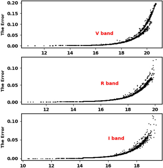
The VRI errors of the observed magnitudes for the stars of King 18.
Gaia DR3 data
We extract the archived data of King 18 from Gaia (Gaia DR3)27. This database consists of positions on the sky (, ), proper motions (cos, ), and parallaxes with a limiting magnitude of G = 21 mag. Gaia DR3 provides astrophysical parameters for many celestial objects derived from parallaxes, broadband photometry, and mean radial velocity spectra. In Gaia DR3, the trigonometric parallax errors are 0.02-0.07 milliarcsecond (mas) for sources at G 17 mag, 0.5 mas for G = 20 mag and reach 1.3 mas for G = 21 mag. The proper motion errors are 0.02-0.07 mas , reaching up to 0.5 mas for G = 20 mag and 1.4 mas for G = 21 mag. Moreover, it contains G magnitudes for around 1.806 billion sources and and magnitudes for around 1.542 billion and 1.555 billion sources, respectively. Fig. 2 shows the number surface density of King 18 from Gaia DR3 and Fig. 3 shows the proper motions cos, and parallax histograms.
Figure 2.
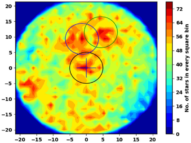
The number surface density of King 18 using the data of Gaia DR3. The cross-hairs represent the center of King 18 cluster. The green and blue circles are stars batches around the cluster. They might be companions to King 18 (the running future work).
Figure 3.

The proper motion in right ascension, declination, and parallax in the field of King 18.
2MASS data
In this section, we have used the Two Micros All-sky Survey (2MASS28) data for the cluster King 18. This data set uses two highly automated 1.3 m telescopes, one at Mt. Hopkins, Arizona (AZ), USA and the other at CTIO, Chile, with a 3-channel camera (256 256 array of HgCdTe detectors in each channel). The 2MASS catalog provides J (1.25 m), H (1.65 m) and (2.17 m) band photometry for millions of galaxies and nearly a half-billion stars. The sensitivity of this catalog is 15.8 mag for J, 15.1 mag for H and 14.3 mag for band at S/N =10.
VRI photometric observations
The 74-inch telescope of the KAO, was utilized to make the VRI CCD photometric observations of King 18, that are used in this investigation. The observation has been secured in the Newtonian focus with a plate scale of 22.53 arcsec/mm and field area of 10 10 on the night of August 27, 2014. The different characteristics of the CCD Camera used in KAO are explained in details, see29.
The numbers of observed stars in V, R, and I bands are 1772, 2576, and 3910, respectively. The mean error for each band is found to be 0.027, 0.024 and 0.023, respectively.
Photometric calibration
For calibration purposes, the observational raw data of king 18 was observed by the f/4.9 Newtonian focus of 74-inches KAO telescope. In addation, there are 9 dome flats for every filter and 10 bias frames. The Processing and analysis of the data were done by Python programming language, utilizing several modules and SExtractor function30. First of all, we began the processing by using the ccdproc package31, which is an Astropy-affiliated package. This process included bias subtraction, flat field correction and cosmic ray removal with the L.A.Cosmic algorithm in the lacosmic Python package32. The stars have been detected by using the SExtractor and then Astropy package33 is applied. Using the background estimated map for each frame, the Photutils package, which offers tools for photometry of astronomical sources34, is applied to obtain instrumental magnitudes. Next, we added World Coordinate System (WCS) information to each frame using the Astrometry.net tool35. This is important because it allows us to cross-match the sources with catalog data for additional calibration.
Finally, STDPipe36, a suite of Python scripts designed for astrometry, photometry, and transient detection tasks in optical imagery, was employed to compute the calibrated magnitudes for all stars within the observed field. The detected stars were matched with Pan-STARRS1 (PS1) catalogue37 and then the photometric model for their instrumental magnitudes was built. This photometric model for the calibrated magnitudes, , was defined as follows, based on36:-
| 1 |
Here, is the instrumental magnitude of the source measured by the detector, ZP is the spatially varying zero-point function, and C is a color-correction term to account for the color distribution of the PS1 calibration stars and the resulting errors are shown in Fig. 1. In this work, the magnitudes of PS1 stars are converted to Johnson-Cousins filters (UBVRI) by using equations of38.
Cluster density profile and radius
To study the cluster structure and to construct radial density profile, the first step is to find rigorously the cluster center. Our major goal is to estimate the highest central density of stars in the cluster. Subsequently, we have created the two dimensional-histogram of star counts in both right ascension () and declination () using the Gaia DR3 database. We used the function histogram2d in numpy package and found the cell with maximum stars. We repeated the process in “Proper motion, membership determination and cluster center”, this time focusing solely on member stars, and discovered no difference.
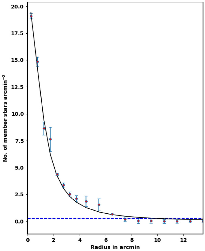
To appraise the cluster extent, we construct the radial density profile (RDP) of King 18 through splitting its observed area into concentric circles. The number of stars is counted in every shell or ring as , then the star number density is calculated as where is the ring or shell area ( ) and and represent the inner and outer radius. The RDP is presented in Fig. 4, where the black solid line shows the fitted King model of39. Thus the density function f(r) is expressed as :
| 2 |
where , , and are the core radius, the background density, and the central density of the cluster, respectively. By fitting the King model to the RDP f(r), we can evaluate the structural parameters for King 18. The blue dashed line in Fig. 4 shows the background density () that is found to be 26.93 ± 0.25 stars . The calculated values of the central density, the core radius and the border radius (R) are 21.06 ± 2.20 stars , 1.05 ± 0.02 arcmin and 7.90 ± 0.21 arcmin, respectively, (see Table 1). The error of fitted parameters is calculated by using covariance matrix of curve_fit function in Scipy package (https://scipy.org/).
Figure 4.
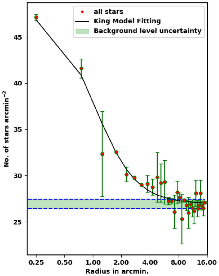
The radial density profile (RDP) of King 18.
Table 1.
King model fit parameters.
| Name | radius | ||||
|---|---|---|---|---|---|
| King 18 | 21.06 ± 2.20 | 26.93 ± 0.27 | 1.05 ± 0.02 | 1.78 | 7.90 ± 0.21 |
Another important parameter for the cluster is the star density contrast parameter, which is expressed as :-
| 3 |
For King 18, the contrast parameter value is 1.75 which is smaller than the values () calculated for compact star clusters, as given by40. This means that King 18 is a sparse cluster.
We have estimated the cluster tidal radius according to the formula of41 :
| 4 |
where and are the tidal radius and total cluster mass, respectively. Our estimated value for the cluster tidal radius is 11.49 pc, where the total cluster mass is 487.39 , see “The cluster mass”. This value is very high and we think the formula of41 is missing some masses compared to Gaia DR3 era (Gaia has higher limiting magnitude with wider G band).
There is another parameter in literature which is called limiting radius of cluster , that was introduced by42. The cluster limiting radius, , is calculated by comparing f(r) to a border background density level, , defined as:
| 5 |
where is the uncertainty of . The is calculated according to the following formula :
| 6 |
For our cluster King 18, this value is about 2.20 arcmin which is an unrealistic value. Moreover, the last equation (intrinsic value for cluster) depends on of the background and foreground stars which is non physical.
Proper motion, membership determination and cluster center
The determination of essential parameters of a cluster is affected by the contamination due to field stars. The membership determination of stars in star clusters was carried out in previous years through photometric and kinematic data43–45. Recently, the astrometric data from Gaia survey has made the kinematic method of membership determination more trustworthy. Proper motion and parallax are very precious agents to separate field stars from the cluster zone, as cluster stars have similar kinematical properties and distances46. We have used Gaia DR3 proper motion and parallax data to separate cluster star members from non members.
The Unsupervised Photometric Membership Assignment in Stellar Clusters algorithm (UPMASK), originally presented in47, has the advantage of being not only non-parametric, but also unsupervised.This means that no prior selection of field stars is necessary in order to serve as a comparison model. The pyUPMASK python package (https://github.com/msolpera/pyUPMASK)48 is an improved version of the original UPMASK algorithm. It relies on the Python library scikit-learn49 (https://scikit-learn.org/stable/) for the implementation of most of the supported clustering methods (https://github.com/adamdempsey90/StarClusters). This library includes around a dozen of different clustering methods for unlabeled data, which are all available to use in the pyUPMASK.
We have used the pyUPMASK python package for finding the membership probability. We have fed it with Gaia DR3 data, about 21926 stars within . Fig. 5 plots the total number of stars (N(P)) as a function of membership probability. From the fitting of King profile (“Cluster density profile and radius”), we get the total number of member stars as 307, which corresponds to a probability that is larger than 94%. This probability value is high because of contamination of the crowded field stars.
Figure 5.
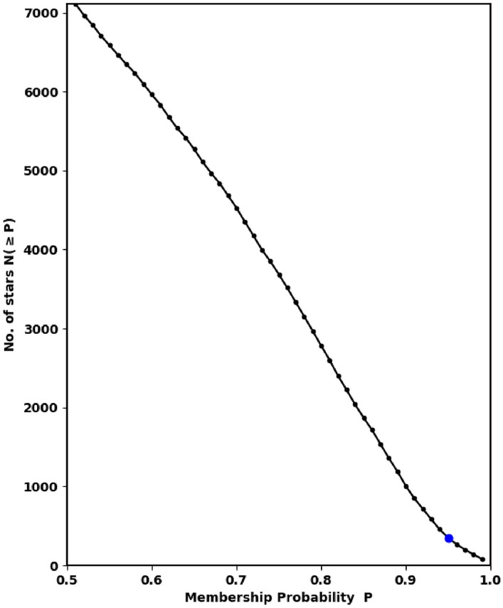
The number of stars as function of membership probability, the output of pyUPMask code.
We have determined the cluster parameters by averaging the values of member stars with probability greater than 98% within 5 arcmin radius, to get more accuracy. The cluster center is found at ; and ; , which is corresponding to galactic l and b (, ). In addition, the values of and are -2.603 ± 0.018 and -2.106 ± 0.013, respectively.
The average value of parallax () is found to be 0.324 ± 0.040 mas. Thus the cluster distance () that corresponds to parallax, is 3.086 ± 0.038 kpc, which is in good agreement with our photometric data results within the errors, see Table 2 for tabulated results.
Table 2.
The center’s coordinates of King 18.
| Name | l | b | |||||
|---|---|---|---|---|---|---|---|
| Unit | Degrees | Degrees | mas | mas | mas | Degrees | Degrees |
| King 18 | 343.044 ± 0.048 | 58.289 ± 0.032 | -2.603 ± 0.018 | -2.106 ± 0.013 | 0.324 ± 0.040 | - |
Other important parameter is the angle which is the angle or direction of cluster movement in and space and is given by, see Fig. 7:
| 7 |
Cluster member stars will move nearly with the same direction through space. Figure 6 shows the histogram for member stars with average angle about , which is more clear than Fig. 7. Moreover, dispersion in histogram depends on cluster age and how strongly the cluster is bound.
Figure 7.
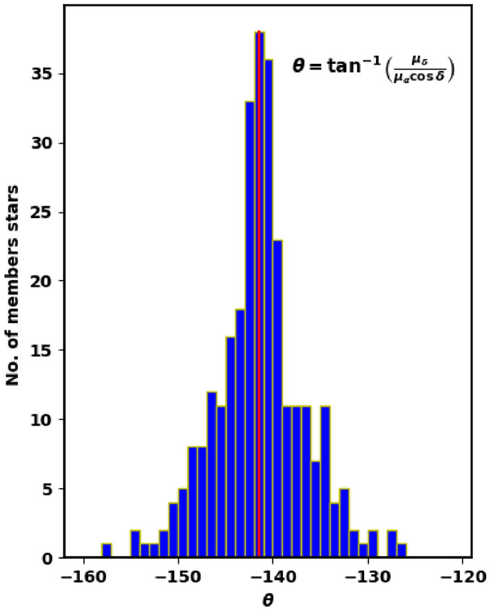
The histogram for member stars.
Figure 6.
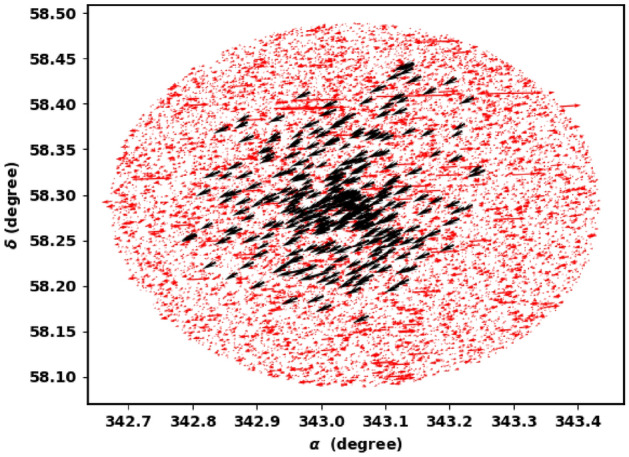
The co-moving stars of King 18 from Gaia DR3.
Test of members’ separation method
In literature, the probability cut-off of member stars is often taken at 50% which is not correct. The probability cut-off value depends on the used method itself, as the density of the field and the distance between the star and the cluster’s center. Critically, the choice of the probability cut-off value must be carefully tested, otherwise we will get wrong member stars. On the other hand, the fitted King profile model can play important role in this context
To test the probability cut-off value and the vitality of members’ separation method, we plot again the stellar density profile, but for member stars only as shown in Fig. 8. This result is very satisfactory and agrees with King profile. The King density profile can constrain both the vitality of membership separation method and the total number of member stars in the cluster. On the contrary, if the membership separation method or probability cut-off value are not correct, we will get member stars over or under estimation. As example, if the probability cut-off value is 80%, we will get overestimated member stars, as seen in Fig. 9. In future work, we will address this point in more detail.
Figure 8.
The stellar density profile of member stars. The solid line is the fitted King profile. The red dots are star density counts of member stars with probability of 94%.
Figure 9.
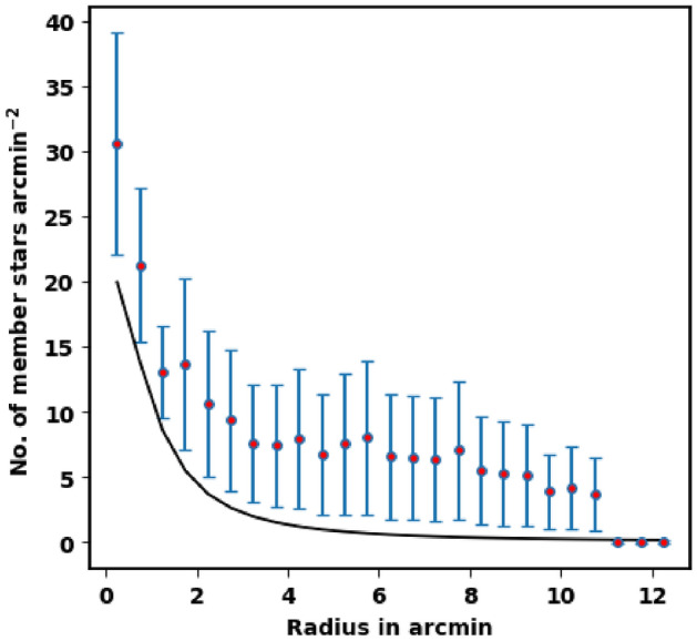
The cluster stellar density at probability cut-off value 80%. The members at this probability cut-off are much over King model function which are overestimated.
The color magnitude diagrams and cluster age
Color-magnitude diagrams (CMDs) of OCs introduce empirical isochrones to compare with the theoretical models of stellar evolution50,51. CMDs are efficient tools to estimate distance, age, and metallicity of an open cluster. Moreover, comparing the observed CMDs with the theoretical isochrones can also give wealth of information about masses of stars in an open cluster. The theoretical isochrones are downloaded from the CMD 3.7 web site (http://stev.oapd.inaf.it/cgi-bin/cmd) using PARSEC version 1.25 s52.
Extinction
A precise interstellar dust extinction law is critically important to interpret observations. Extinction coefficients per passbands depend on the source spectral energy distribution, interstellar matter and on the extinction itself. Both the color excess ratio (CER) E()/E() and the relative extinction are indicators of the extinction law. Following the method presented in53, we compute the extinction coefficient in the Gaia and 2MASS bands by using the relation , as an example , and . For 2MASS, , and .
For VRI observations, we use values of the extinction law of54,55, which are , , and . Then we can get the relation between extinction and color excess as follow:
From isochrone fitting we are able to estimate the color excess and finally extinction. By using the following equation the intrinsic distance modulus can be calculated :
| 8 |
where m is the apparent absorbed magnitude, M is the absolute magnitude and is the extinction in band.
The CMD Of Gaia DR3 data
By using the photometric data extracted from Gaia DR3 of stars of King 18, the CMD is plotted in Fig. 10. The CMD is fitted by the theoretical isochrones of50.
Figure 10.
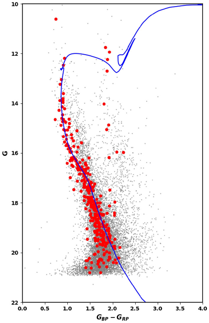
The color magnitude diagram (CMD) for the clusters’ members of King 18 using the photometric bands (G, & ) of the Gaia DR3.
We have found that the observed distance modulus and the color excess E(–) are 14.20 ± 0.80 mag and 0.98 ± 0.13 mag, respectively. To obtain the distance modulus and the extinction in G band , we used the equation in “Extinction”. These values are found to be 12.38 and 1.82, respectively, which is corespondent to the distance of 2992.0 ± 47 pc. Moreover the fitted isochrone produces a cluster age of about 224 ± 6.3 Myr, at Z = 0.0152. Figure 10 shows the CMD of King 18 using the wide photometric bands (G, & ) of the Gaia DR3 database.
The CMD of 2MASS data
Using the intersect1d function in the Python Numpy package (https://numpy.org/)56, we have matched member stars discovered in Gaia DR3 with 2MASS data. We found 231 member stars in both databases. The CMD of matched 2MASS data can check the vitality of membership separation method. Next, we plot the CMDs as shown in Fig. 11. From isochrone fitting, we obtain the color excess values of and as 0.380 ± 0.091 and 0.260 ± 0.036, respectively. Additionally, in J band is 12.880 ± 0.202. According to equations in “Extinction ”, we get the value as 0.560 ± 0.081. At the end, the distance modulus is found to be 12.320 ± 0.107, which is corresponding to the distance value of 2910.00 ± 36.50 Pc. This value is in excellent agreement with Gaia parallax and photometry parameters.
Figure 11.

Left: the CMD and J- fit isochrone. Right: the J and J-H one.
The CMD of VRI observation
Additionally, we cross-matched member stars identified by CCD VRI observations and Gaia. In both of them, we have found 278 stars, which is more than the outcome of cross-matching 2MASS and CCD VRI observations (231 stars). For isochrone fitting, we plot CMD V and (V–I) as in Fig. 12. We have found that the apparent distance modulus and color excess E(V–I) are 14.4 and 0.85 , respectively.
Figure 12.

The color magnitude diagram (CMD) for the clusters’ members of King 18 using the photometric bands of VRI Observations.
Using relationship in “Extinction”, the extinctions are found as , and . Next, we obtain the intrinsic distance modulus , that corresponds to the distance of 2857.5 pc. Moreover the age of used isochrones for fitting is myr. At the end, the data reduction and analysis results of Gaia DR3, VRI observations and 2MASS are in agreement with each others within small errors.
Luminosity, the cluster mass, mass functions and dynamical state
Luminosity function
It is clear that luminosity and mass functions (LF & MF) are fundamentally dependent on the cluster’s membership. To remove field stars contamination completely from the main sequence stars of King 18, we used probable cluster members selected by using pyUPMASK python package. After that, we used the photometric data to obtain LF before estimating the MF. For the LF, we converted the apparent G magnitude of member stars into absolute magnitude. Then, we plot histograms (Fig. 13) showing the LF of King 18.
Figure 13.
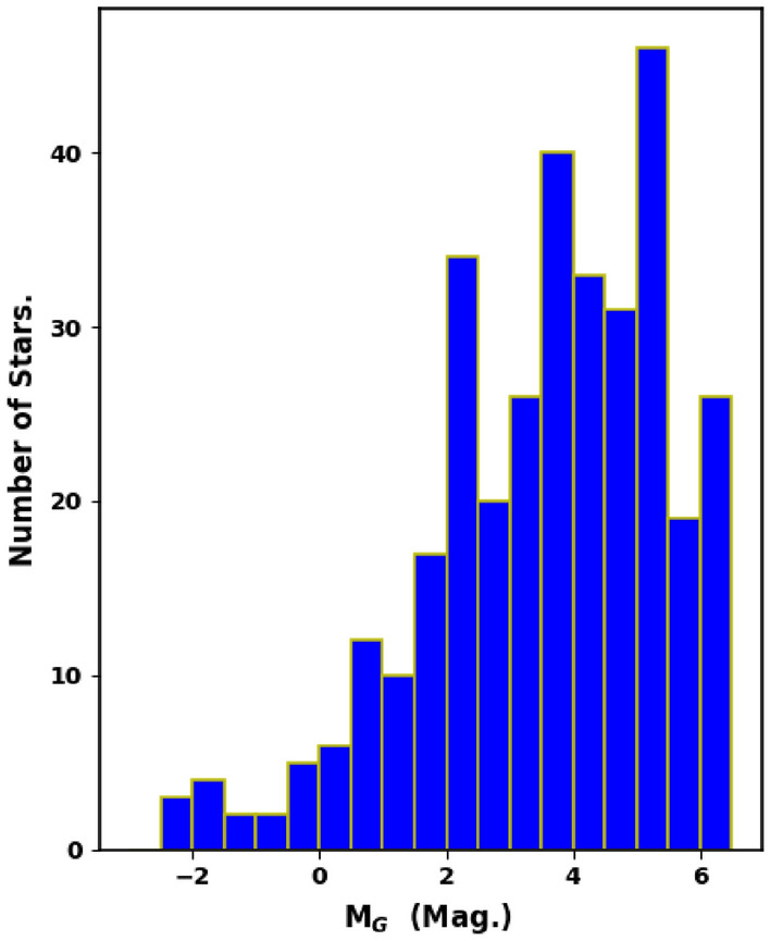
The luminosity function (LF) of King 18 with bin interval of 0.5 mag.
The cluster mass
It is obvious that the individual star mass in a cluster is a very important parameter in addition to the total cluster mass as well. After making isochrone fitting, we get the absolute magnitude and the intrinsic color . The mass obtained by the normal polynomial fitting is incorrect and yields misleading values. We need an interpolation routine with two independent variables. So we have used SmoothBivariateSpline routine in Python Scipy (https://scipy.org/) package57 which uses two variables for interpolation because the star mass depends on magnitude and color as well.
We have used and as two independent interpolation variables from the best isochrone fit. By this way, we obtain the individual mass of every member star. Now, we are able to get the total cluster mass with high accuracy, 487.39 . Also we obtain the cluster mass profile as shown in Fig. 15. Moreover, we get pc, within which half of the cluster mass is included, see Eq. (10).
Figure 15.
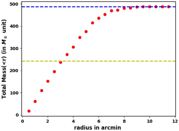
The mass profile M(<r) of King 18. The horizontal blue dashed line represents total mass and yellow dashed one represents the half cluster mass at .
Mass function
The mass function (MF) can be defined as the distribution of masses of cluster’s stars per unit volume during the time of star formation. We can convert LF into MF by using a mass-luminosity relation. As we can not get an observational transformation, we must rely on theoretical models. In order to transform LF into MF, we use the theoretical isochrones of50,58. The topic concerning the initial mass function (IMF), whether it is universal in time and space or it depends on conditions of star formation, represents a current mystery59–61. Also, The study of mass-segregation in OCs provides an evidence for the distribution of low and high mass stars towards the cluster region. The IMF can be expressed as;
| 9 |
where, is the number of stars that has a mass interval from M to M + dM, and is the slope of the mass function. The value of is found to be 2.27 ± 0.17 (see Fig. 14), which is in agreement with Salpeter value62.
Figure 14.
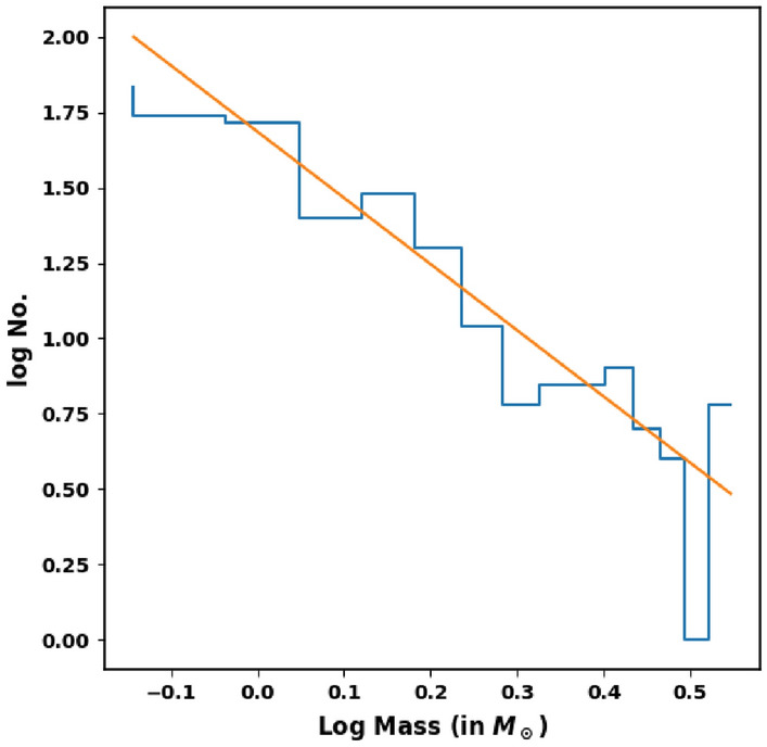
The initial mass function (IMF) of King 18.
Dynamical state
Another important parameter that is used to understand the dynamical evolution of a star cluster, is the relaxation time. It is the time scale in which the cluster will lose all its traces of initial conditions and its member stars will have a roughly Maxwellian distribution of velocities. According to63, the relaxation time is explained by,
| 10 |
where N denotes for the number of cluster members, is the radius in pc, within which half of the cluster mass is included, and m is the average mass of the cluster in solar units. In Fig. 15, we plot the mass inside radius r. From this figure, we found the value of equals 3.11 arcmin (2.73 pc). By applying the above equation, we found that the relaxation time of King 18 equals 28.92 Myr which is much younger than the cluster age (224–251 Myr). That means that King 18 is dynamically stable and a relaxed cluster. Table 3 presents our results including all the calculated astrophysical parameters of Kink 18, in addition to a comparison with previous studies.
Table 3.
Comparison between parameters of the open cluster King 18 in the current study and literature.
| Parameter | Gaia DR3 | Present work | 24 | 25 | 26 |
|---|---|---|---|---|---|
| VRI photometric observations | |||||
| Radius (arcmin) | 7.90 ± 0.21 | 9.50 ± 0.40 pc | 4.80 | 8.00 | |
| Members | 307 | 2400 | |||
| + | + 00 | + | + 36 | ||
| cos(mas/yr) | -2.603 ± 0.018 | ||||
| (mas/yr) | -2.106 ± 0.013 | ||||
| Parallax (mas) | 0.324 ± 0.040 | ||||
| E(B–V) (mag) | 0.63 ± 0.01 | 0.52 | 0.69 ± 0.04 | ||
| E(V–I) (mag) | 0.850±0.087 | ||||
| E(R–I) (mag) | 0.45 | ||||
| E(–) (mag) | 0.98 ± 0.13 | ||||
| Age (Myr) | 224 ± 6.3 | 224 ± 6.3 | 251.2 | 350 | 130 ± 10 |
| Distance modulus (mag) | 12.38±1.32 | 12.28 ±0.29 | 13.85 | 11.8 | 12.39 ± 0.21 |
| Total mass () | 487.39 | 1050 | |||
| MF slope | 2.27±0.17 | 0.90 ± 0.50 | |||
| Relaxation time (Myr) | 28.92 |
Summary and conclusions
We performed a study on the young open cluster King 18 based on Gaia DR3 photometric and astrometric data, and the VRI CCD photometric observations using the f/4.9 74-inch telescope at Kottamia Astronomical Observatory (KAO). According to our analysis for refining the fundamental parameters of King 18 in the Gaia era DR3 and VRI CCD observations, we presented a detailed astro-photometric study here, which is somehow different from the previous results. The main results of our analysis are as follow :
The slope value of King 18 mass function () is found to be 2.27, which is in agreement with Salpeter value62. Based on our data of KAO and that of Gaia DR3, we have estimated the cluster age to be 224 ± 6.3 Myrs, and the relaxation time is 28.92 Myr. That means that King 18 is dynamically stable and relaxed cluster.
The cluster distance modulus from Gaia, 2Mass and VRI observations has been determined to be 12.38 ± 1.32, 12.32 ± 0.11 and 12.28 ± 0.29 mag respectively, which corresponds to distances of 2992.26, 2910.72 and 2857.59 pc, respectively. These results are in good agreement within the error. Moreover the color excess E(V–I), E(J–) and E(–) are 0.85 ± 0.09, 0.38 ± 0.09 and 0.98 ± 0.13, respectively.
The values of proper motion (cos, ), and parallaxes () are , and respectively. The cluster distance corresponding to parallax () is 3.236 ± 0.500 kpc which is in good agreements with our photometric data result within the errors.
Finally, the present and previous results are summarized and compared with others in Table 3.
Acknowledgements
The authors are grateful to Prof. Charles Bunatto, UFRGS, Porto Alegre, Rio Grande do Sul, Brazil for his insightful feedback and productive conversations about this research. Authors thank Prof. Ashraf Tadross, NRIAG, for useful comments and fruitful discussions regarding this study. Authors also acknowledge Prof. Mashhoor Ahmad Al-Wardat, College of Sciences, University of Sharjah, for his helpful comments about this study. This work has made use of data from the European Space Agency (ESA) space mission Gaia. Gaia data are being processed by the Gaia Data Processing and Analysis Consortium (DPAC). Funding for the DPAC is provided by national institutions, in particular the institutions participating in the Gaia MultiLateral Agreement (MLA). The Gaia mission website is https://www.cosmos.esa.int/gaia. The Gaia archive website is https://archives.esac.esa.int/gaia. The authors are pretty thankful to Python community for large efforts especially for Matplotlib, Numpy, Scipy and Astropy etc. groups. Their efforts contributed to making data analysis easier as well as representing it graphically in a creative way.
Author contributions
Nasser M. Ahmed: Gaia data analysis and writing. R. M. Samir: 2Mass data analysis and writing. R. Bendary and E. G. Elhosseiny: VRI observations and their data reduction.
Funding
Open access funding provided by The Science, Technology & Innovation Funding Authority (STDF) in cooperation with The Egyptian Knowledge Bank (EKB).
Data availability
Our VRI CCD observations: are available upon request from any of the authors (nasser_ahnmed@yahoo.com) Gaia and 2Mass data: are available for free in webpage https://vizier.cds.unistra.fr/ .
Competing interests
The authors declare no competing interests.
Footnotes
Publisher's note
Springer Nature remains neutral with regard to jurisdictional claims in published maps and institutional affiliations.
References
- 1.Lada, C. J. & Lada, E. A. Embedded clusters in molecular clouds. Annu. Rev. Astron. Astrophys.41, 57–115. 10.1146/annurev.astro.41.011802.094844 (2003) arXiv:astro-ph/0301540. [Google Scholar]
- 2.Carraro, G., Geisler, D., Villanova, S., Frinchaboy, P. M. & Majewski, S. R. Old open clusters in the outer Galactic disk. Astron. Astrophys.476, 217–227. 10.1051/0004-6361:20078113 (2007) arXiv:0709.2126. [Google Scholar]
- 3.Cantat-Gaudin, T. & Anders, F. Clusters and mirages: Cataloguing stellar aggregates in the Milky Way. Astron. Astrophys.633, A99. 10.1051/0004-6361/201936691 (2020) arXiv:1911.07075. [Google Scholar]
- 4.Madore, B. F., Freedman, W. L., Lee, A. J. & Owens, K. Milky Way zero-point calibration of the JAGB method: Using thermally pulsing AGB stars in galactic open clusters. Astrophys. J.938, 125. 10.3847/1538-4357/ac92fd (2022) arXiv:2209.08127. [Google Scholar]
- 5.van den Bergh, S. Diameters of open star clusters. Astronomy131, 1559–1564. 10.1086/499532 (2006) arXiv:astro-ph/0511702. [Google Scholar]
- 6.Dias, W. S., Monteiro, H., Lépine, J. R. D. & Barros, D. A. The spiral pattern rotation speed of the Galaxy and the corotation radius with Gaia DR2. Mon. Not. R. Astron. Soc.486, 5726–5736. 10.1093/mnras/stz1196 (2019) arXiv:1905.08133. [Google Scholar]
- 7.Bobylev, V. V. & Bajkova, A. T. Determination of the spiral pattern speed in the Milky Way from young open star clusters. Astron. Lett.49, 320–330. 10.1134/S1063773723060014 (2023) arXiv:2309.12097. [Google Scholar]
- 8.Friel, E. D. The old open clusters of the Milky Way. Annu. Rev. Astron. Astrophys.33, 381–414. 10.1146/annurev.aa.33.090195.002121 (1995). [Google Scholar]
- 9.Randich, S. & Gilmore, G. Gaia-ESO Consortium. The Gaia-ESO large public spectroscopic survey. Messenger154, 47–49 (2013). [Google Scholar]
- 10.Krumholz, M. R., McKee, C. F. & Bland-Hawthorn, J. Star clusters across cosmic time. Annu. Rev. Astron. Astrophys.57, 227–303. 10.1146/annurev-astro-091918-104430 (2019) arXiv:1812.01615. [Google Scholar]
- 11.Salaris, M., Weiss, A. & Percival, S. M. The age of the oldest open clusters. Astron. Astrophys.414, 163–174. 10.1051/0004-6361:20031578 (2004) arXiv:astro-ph/0310363. [Google Scholar]
- 12.Magrini, L., Sestito, P., Randich, S. & Galli, D. The evolution of the galactic metallicity gradient from high-resolution spectroscopy of open clusters. Astron. Astrophys.494, 95–108. 10.1051/0004-6361:200810634 (2009) arXiv:0812.0854. [Google Scholar]
- 13.Netopil, M., Paunzen, E., Heiter, U. & Soubiran, C. On the metallicity of open clusters. III. Homogenised sample. Astron. Astrophys.585, A150. 10.1051/0004-6361/201526370 (2016) arXiv:1511.08884. [Google Scholar]
- 14.Donor, J. et al. The open cluster chemical abundances and mapping survey. IV. Abundances for 128 open clusters using SDSS/APOGEE DR16. Astronomy159, 199. 10.3847/1538-3881/ab77bc (2020) arXiv:2002.08980. [Google Scholar]
-
15.Tognelli, E., Dell’Omodarme, M., Valle, G., Prada Moroni, P. G. & Degl’Innocenti, S. Bayesian calibration of the mixing length parameter

 and of the helium-to-metal enrichment ratio
  Y/
Y/ Z with open clusters: The Hyades test-bed. Mon. Not. R. Astron. Soc.501, 383–397. 10.1093/mnras/staa3686 (2021) arXiv:2012.08193. [Google Scholar]
 - 16.Alonso-Santiago, J. et al. High-resolution spectroscopy of the young open cluster M 39 (NGC 7092). Astron. Astrophys.683, A75. 10.1051/0004-6361/202348483 (2024) arXiv:2312.08581. [Google Scholar]
- 17.Dias, W. S., Alessi, B. S., Moitinho, A. & Lépine, J. R. D. New catalogue of optically visible open clusters and candidates. Astron. Astrophys.389, 871–873. 10.1051/0004-6361:20020668 (2002) arXiv:astro-ph/0203351. [Google Scholar]
- 18.Kharchenko, N. V., Piskunov, A. E., Schilbach, E., Röser, S. & Scholz, R. D. Global survey of star clusters in the Milky Way. II. The catalogue of basic parameters. Astron. Astrophys.558, A53. 10.1051/0004-6361/201322302 (2013) arXiv:1308.5822. [Google Scholar]
- 19.Tadross, A. L. The simplest way to get a cluster’s parameters in the Gaia era (Dolidze 41). Res. Astron. Astrophys.18, 158. 10.1088/1674-4527/18/12/158 (2018) arXiv:1808.01654. [Google Scholar]
- 20.Yontan, T. et al. A Study of Open Clusters Frolov 1 and NGC 7510 using CCD UBV Photometry and Gaia DR2 Astrometry. arXiv e-printsarXiv:2012.12269 (2020).
- 21.Anders, P., Bissantz, N., Fritze, V., Alvensleben, U. & de Grijs, R. Analysing observed star cluster SEDs with evolutionary synthesis models: Systematic uncertainties. Mon. Not. R. Astron. Soc.347, 196–212. 10.1111/j.1365-2966.2004.07197.x. arXiv:astro-ph/0309356 (2004).
- 22.King, I. R., Bedin, L. R., Piotto, G., Cassisi, S. & Anderson, J. Color-magnitude diagrams and luminosity functions down to the hydrogen-burning limit. III. A preliminary hubble space telescope study of NGC 6791. Astronomy130, 626–634. 10.1086/431327 (2005) arXiv:astro-ph/0504627. [Google Scholar]
- 23.King, I. Some new galactic clusters. Harvard Coll. Observ. Bull.919, 41–42 (1949). [Google Scholar]
- 24.Maciejewski, G. Photometric studies of open clusters: Be 95, Cze 21, Cze 38, Ju 11, King 17, and King 18. Acta Astron.58, 389 (2008). [Google Scholar]
- 25.Tadross, A. L. An investigation of 11 previously unstudied open star clusters. New Astron.14, 200–205. 10.1016/j.newast.2008.08.004 (2009) arXiv:0804.2567. [Google Scholar]
- 26.Glushkova, E. V. et al. Photometry of the poorly studied galactic open star clusters King 13, King 18, King 19, King 20, NGC 136, and NGC 7245. Astron. Lett.36, 14–26. 10.1134/S1063773710010032 (2010). [Google Scholar]
- 27.Gaia Collaboration et al. Gaia Data Release 3. Summary of the content and survey properties. Astron. Astrophys.674, A1 10.1051/0004-6361/202243940. arXiv:2208.00211 (2023).
- 28.Skrutskie, M. F. et al. The two micron all sky survey (2MASS). Astronomy131, 1163–1183. 10.1086/498708 (2006). [Google Scholar]
- 29.Azzam, Y. A., Ali, G. B., Ismail, H. A., Haroon, A. & Selim, I. Current and future capabilities of the 74-inch telescope of Kottamia Astronomical Observatory in Egypt. In Third UN/ESA/NASA Workshop on the International Heliophysical Year 2007 and Basic Space Science. Vol. 20. Astrophysics and Space Science Proceedings. 175–187. 10.1007/978-3-642-03325-4_16 (2010).
- 30.Bertin, E. & Arnouts, S. SExtractor: Software for source extraction. Astron. Astrophys. Suppl. Ser.117, 393–404. 10.1051/aas:1996164 (1996). [Google Scholar]
- 31.Craig, M. et al. astropy/ccdproc: v1.3.0.post1. 10.5281/zenodo.1069648 (2017).
- 32.van Dokkum, P. G. Cosmic-ray rejection by Laplacian edge detection. PASP113, 1420–1427. 10.1086/323894 (2001) arXiv:astro-ph/0108003. [Google Scholar]
- 33.Astropy Collaboration et al. The Astropy Project: Sustaining and growing a community-oriented open-source project and the latest major release (v5.0) of the core package. Astrophys. J.935, 167 10.3847/1538-4357/ac7c74. arXiv:2206.14220 (2022).
- 34.Bradley, L. et al. astropy/photutils: 1.5.0. 10.5281/zenodo.6825092 (2022).
- 35.Lang, D., Hogg, D. W., Mierle, K., Blanton, M. & Roweis, S. Astrometry.net: Blind astrometric calibration of arbitrary astronomical images. Astronomy139, 1782–1800. 10.1088/0004-6256/139/5/1782 (2010) arXiv:0910.2233. [Google Scholar]
- 36.Karpov, S. STDPipe: Simple Transient Detection Pipeline. Astrophysics Source Code Library, Record ascl:2112.006 (2021).
- 37.Chambers, K. C. et al. The Pan-STARRS1 Surveys. arXiv e-printsarXiv:1612.05560, 10.48550/arXiv.1612.05560 (2016).
- 38.Kostov, A. & Bonev, T. Transformation of Pan-STARRS1 GRI to Stetson BVRI magnitudes. Photometry of small bodies observations. Bulgar. Astron. J.28, 3. 10.48550/arXiv.1706.06147 (2018) arXiv:1706.06147. [Google Scholar]
- 39.King, I. R. The structure of star clusters. III. Some simple dynamical models. Astronomy71, 64. 10.1086/109857 (1966). [Google Scholar]
- 40.Bonatto, C. & Bica, E. The nature of the young and low-mass open clusters Pismis5, vdB80, NGC1931 and BDSB96. Mon. Not. R. Astron. Soc.397, 1915–1925. 10.1111/j.1365-2966.2009.14877.x (2009) arXiv:0904.1321. [Google Scholar]
- 41.Jeffries, R. D., Thurston, M. R. & Hambly, N. C. Photometry and membership for low mass stars in the young open cluster NGC 2516. Astron. Astrophys.375, 863–889. 10.1051/0004-6361:20010918 (2001) arXiv:astro-ph/0107097. [Google Scholar]
- 42.Bukowiecki, Ł, Maciejewski, G., Konorski, P. & Strobel, A. Open clusters in 2MASS photometry. I. Structural and basic astrophysical parameters. Acta Astron.61, 231–246. 10.48550/arXiv.1107.5119 (2011) arXiv:1107.5119. [Google Scholar]
- 43.Dias, W. S. et al. Proper motions of the optically visible open clusters based on the UCAC4 catalog. Astron. Astrophys.564, A79. 10.1051/0004-6361/201323226 (2014). [Google Scholar]
- 44.Sampedro, L., Dias, W. S., Alfaro, E. J., Monteiro, H. & Molino, A. A multimembership catalogue for 1876 open clusters using UCAC4 data. Mon. N. R. Astron. Soc.470, 3937–3945. 10.1093/mnras/stx1485 (2017) arXiv:1706.05581. [Google Scholar]
- 45.Topasna, G. A., Kaltcheva, N. T. & Paunzen, E. Interstellar polarization and extinction towards the young open cluster NGC 1502. Astron. Astrophys.615, A166. 10.1051/0004-6361/201731903 (2018). [Google Scholar]
- 46.Rangwal, G., Yadav, R. K. S., Durgapal, A., Bisht, D. & Nardiello, D. Astrometric and photometric study of NGC 6067, NGC 2506, and IC 4651 open clusters based on wide-field ground and Gaia DR2 data. Mon. Not. R. Astron. Soc.490, 1383–1396. 10.1093/mnras/stz2642 (2019) arXiv:1909.08810. [Google Scholar]
- 47.Krone-Martins, A. & Moitinho, A. UPMASK: Unsupervised photometric membership assignment in stellar clusters. Astron. Astrophys.561, A57. 10.1051/0004-6361/201321143 (2014) arXiv:1309.4471. [Google Scholar]
- 48.Pera, M. S., Perren, G. I., Moitinho, A., Navone, H. D. & Vazquez, R. A. pyUPMASK: An improved unsupervised clustering algorithm. Astron. Astrophys.650, A109. 10.1051/0004-6361/202040252 (2021) arXiv:2101.01660. [Google Scholar]
- 49.Pedregosa, F. et al. Scikit-learn: Machine learning in Python. J. Mach. Learn. Res.12, 2825–2830. 10.48550/arXiv.1201.0490 (2011) arXiv:1201.0490. [Google Scholar]
- 50.Marigo, P. et al. A new generation of PARSEC-COLIBRI stellar isochrones including the TP-AGB phase. Astrophys. J.835, 77 (2017) arXiv:1701.08510. [Google Scholar]
- 51.Spada, F., Demarque, P., Kim, Y. C., Boyajian, T. S. & Brewer, J. M. The Yale-Potsdam stellar isochrones. Astrophys. J.838, 161. 10.3847/1538-4357/aa661d (2017) arXiv:1703.03975. [Google Scholar]
- 52.Bressan, A. et al. PARSEC: Stellar tracks and isochrones with the PAdova and TRieste stellar evolution code. Mon. Not. R. Astron. Soc.427, 127–145. 10.1111/j.1365-2966.2012.21948.x (2012) arXiv:1208.4498. [Google Scholar]
- 53.Wang, S. & Chen, X. The optical to mid-infrared extinction law based on the APOGEE, Gaia DR2, Pan-STARRS1, SDSS, APASS, 2MASS, and WISE surveys. Astrophys. J.877, 116. 10.3847/1538-4357/ab1c61 (2019) arXiv:1904.04575. [Google Scholar]
- 54.Cardelli, J. A., Clayton, G. C. & Mathis, J. S. The relationship between infrared, optical, and ultraviolet extinction. Astrophys. J.345, 245. 10.1086/167900 (1989). [Google Scholar]
- 55.O’Donnell, J. E. R v-dependent optical and near-ultraviolet extinction. Astrophys. J.422, 158. 10.1086/173713 (1994). [Google Scholar]
- 56.Harris, C. R. et al. Array programming with NumPy. Nature585, 357–362. 10.1038/s41586-020-2649-2 (2020). [DOI] [PMC free article] [PubMed] [Google Scholar]
- 57.Virtanen, P., Fundamental algorithms for scientific computing in Python. SciPy 1.0. Nat. Methods17, 261–272. 10.1038/s41592-019-0686-2 (2020). [DOI] [PMC free article] [PubMed] [Google Scholar]
- 58.Malkov, O., Kovaleva, D., Zhukov, A. & Dluzhnevskaya, O. Theoretical mass-luminosity relations in Gaia G-band. Astrophys. Sp. Sci.367, 37. 10.1007/s10509-022-04066-1 (2022) arXiv:2204.11703. [Google Scholar]
- 59.Kroupa, P. & Boily, C. M. On the mass function of star clusters. Mon. Not. R. Astron. Soc.336, 1188–1194. 10.1046/j.1365-8711.2002.05848.x (2002) arXiv:astro-ph/0207514. [Google Scholar]
- 60.Bastian, N., Covey, K. R. & Meyer, M. R. A universal stellar initial mass function? A critical look at variations. Annu. Rev. Astron. Astrophys.48, 339–389. 10.1146/annurev-astro-082708-101642 (2010) arXiv:1001.2965. [Google Scholar]
- 61.Dib, S. & Basu, S. The emergence of the galactic stellar mass function from a non-universal IMF in clusters. Astron. Astrophys.614, A43. 10.1051/0004-6361/201732490 (2018) arXiv:1711.07487. [Google Scholar]
- 62.Salpeter, E. E. The luminosity function and stellar evolution. Astrophys. J.121, 161. 10.1086/145971 (1955). [Google Scholar]
- 63.Spitzer, J., Lyman & Hart, M. H. Random gravitational encounters and the evolution of spherical systems. I. Method. Astrophys. J.164, 399. 10.1086/150855 (1971).
Associated Data
This section collects any data citations, data availability statements, or supplementary materials included in this article.
Data Availability Statement
Our VRI CCD observations: are available upon request from any of the authors (nasser_ahnmed@yahoo.com) Gaia and 2Mass data: are available for free in webpage https://vizier.cds.unistra.fr/ .