Bayesian Lookahead Perturbation Policy for Inference of Regulatory Networks

Abstract

The complexity, scale, and uncertainty in regulatory networks (e.g., gene regulatory networks and microbial networks) regularly pose a huge uncertainty in their models. These uncertainties often cannot be entirely reduced using limited and costly data acquired from the normal condition of systems. Meanwhile, regulatory networks often suffer from the non-identifiability issue, which refers to scenarios where the true underlying network model cannot be clearly distinguished from other possible models. Perturbation or excitation is a well-known process in systems biology for acquiring targeted data to reveal the complex underlying mechanisms of regulatory networks and overcome the non-identifiability issue. We consider a general class of Boolean network models for capturing the activation and inactivation of components and their complex interactions. Assuming partial available knowledge about the interactions between components of the networks, this paper formulates the inference process through the maximum aposteriori (MAP) criterion. We develop a Bayesian lookahead policy that systematically perturbs regulatory networks to maximize the performance of MAP inference under the perturbed data. This is achieved by optimally formulating the perturbation process in a reinforcement learning context and deriving a scalable deep reinforcement learning perturbation policy to compute near-optimal Bayesian policy. The proposed method learns the perturbation policy through planning without the need for any real data. The high performance of the proposed approach is demonstrated by comprehensive numerical experiments using the well-known mammalian cell cycle and gut microbial community networks.

I. Introduction

Accurate modeling of regulatory networks is critical for a deep understanding of complex biological systems’ mechanisms and harnessing their potential. For instance, in genomics, gene regulatory networks (GRNs) consist of a number of interacting genes, where proper modeling of their activities is crucial for a detailed grasp of various cellular processes (e.g., complex diseases such as cancer) [1]–[3]. Another example is metagenomics, where microbial communities are modeled as regulatory networks comprised of a number of microbes, genes, and metabolites interacting in a tortuous and uncertain fashion. Accurate modeling of microbial communities could help protect humans or plants against diseases or develop next-generation biofuels and biological remediation systems needed for sustainable growth [4]–[8].

Understanding the underlying mechanism of regulatory networks through data acquired from their normal conditions is challenging and, in most cases, impossible. A major reason is that data are often limited or collected in a way that does not elicit the interactions between components. This is typically due to the fact that the network is being trapped in attractor states, which precludes the observation of the entire state-space. This leads to the issue of statistical non-identifiability, which refers to the situation where multiple models are not clearly distinguishable using the available data. Perturbation or excitation is a well-known approach in systems biology that aims to make minimum changes in systems and acquire the most informative data. In regulatory networks, perturbations are often mutations or drug treatments that lead to changes in the expression profile to help understand their underlying mechanisms.

In practice, the perturbations are often selected through a trial-and-error process by biologists or microbiologists due to the lack of appropriate tools for making such decisions. The experts’ decisions are often sub-optimal and inefficient due to the complex and uncertain nature of most practical biological systems. Some attempts have been made toward achieving systematic perturbation of regulatory networks. These include perturbation strategies for static networks [9]–[12], networks modeled by ordinary differential equations (ODE) [13], [14], and deterministic regulatory network models [15], [16]. However, these methods cannot be applied (or perform poorly) in practical biological systems. This is primarily due to their lack of scalability, reliance on heuristics, and unrealistic assumptions (e.g., ignoring dynamics of regulatory networks and modeling them as static networks). In [17], we developed an optimal finite-horizon perturbation policy for small regulatory networks with a small number of unknown interactions and short horizons. This method conducts an exhaustive search over all possible models and state transitions; thus, its applications are limited.

This paper develops a scalable and efficient perturbation method for acquiring data needed for quick and accurate inference of regulatory networks. First, we model regulatory networks with a general class of Boolean network models. Given that the incomplete information about regulatory networks is unknown interactions between components, the objective is to find the best perturbation at any given time that leads to inferring the true model more confidently among the other models. Without loss of generality, we employ the maximum aposteriori (MAP) as an inference criterion. We optimally formulate the perturbation problem in a reinforcement learning context through: 1) defining the joint system’s state and posterior of unknown interactions as a belief state (a sufficient statistic for the perturbation process) and mapping the unknown Boolean process into a Markov decision process (MDP); 2) expressing changes in the maximum posterior of system models, which is a measure of improvement in the inference accuracy, as an immediate reward function. The concept of belief state and the mathematical structure of regulatory networks are used to derive a near-optimal Bayesian perturbation policy. The proposed approach learns the perturbation policy, which yields the Bayesian optimality with respect to the system uncertainty. We demonstrate the high performance of the proposed policy using a mammalian cell cycle in gene regulatory networks and, furthermore, through experiments on a gut microbial community.

The remainder of this paper is organized as follows. Section II provides a detailed description of the regulatory network model. The problem formulation is described in Section III. Section IV includes full details of the proposed perturbation policy and its algorithm. Further, Section V consists of comprehensive numerical experiments on two well-known regulatory networks. Finally, the main conclusions are discussed in section VI.

II. Regulatory Network Model

Without loss of generality, this paper employs a Boolean network with perturbation (BNp) model for capturing the dynamics of regulatory networks [18]–[20]. This model properly captures the stochasticity in regulatory networks, coming from intrinsic uncertainty or unmodeled parts of systems. Consider a regulatory network consisting of $d$ components. The system’s state at time step $k$ can be expressed as a state vector ${\mathbf{X}}_k\in \{\mathrm{0,1}{\}}^d$, which represents the activation/inactivation states of the system’s components. Each component’s state is updated at each discrete time through the following Boolean signal model [21], [22]:

$$X_k=f\left(X_{k-1}\right)\oplus n_k\oplus u_{k-1},$$ (1)

for $k=\mathrm{1,2},\dots$, where ${\mathbf{n}}_k\in \{\mathrm{0,1}{\}}^d$ is Boolean transition noise at time $k,{\mathbf{u}}_{k-1}\in 𝒰\subset \{\mathrm{0,1}{\}}^d$ is the perturbation at time step $k-1,“\oplus ”$ indicates component-wise modulo-2 addition, and f represents the network function. The way that the perturbation impacts the system’s state is by flipping the value of specific components’ states. For instance, ${\mathbf{u}}_{k-1}\left(i\right)=1$ flips the state value of the $i$th component, contrary to the case with ${\mathbf{u}}_{k-1}\left(i\right)=0.$

The network function in (1) is expressed in component form as $\mathbf{f}=\left(f_1,\dots ,f_d\right)$, where each component $f_i:\{\mathrm{0,1}{\}}^d\to \{\mathrm{0,1}\}$ is a Boolean function given by [23]:

$$f_i\left(x\right)=\{\begin{array}{ll}1,\hfill & {\sum }_{j=1}^d{r}_{ij}x\left(j\right)+e_i>0,\hfill \\ 0,\hfill & {\sum }_{j=1}^d{r}_{ij}x\left(j\right)+e_i\le 0,\hfill \end{array}$$ (2)

where $r_{ij}$ denotes the type of regulation from component $j$ to component $i$; it takes +1 and −1 values if there is a positive and negative regulations from component $j$ to component $i$ respectively, and 0 if component $j$ is not an input to component $i$. $e_i$ is a tie-breaking parameter for component $i$; it takes $\frac{+1}{2}$ if an equal number of positive and negative inputs lead to state value +1 and reverse for $\frac{-1}{2}$.

The network function in (2) can also be expressed in matrix form as:

$$f\left(X_{k-1}\right)=\overline{R{X}_{k-1}+e},$$ (3)

where the threshold operator $\stackrel{-}{\mathrm{v}}$ maps the positive elements of vector v to 1 and negative elements to 0, $\mathbf{R}$ is the connectivity matrix with $(\mathbf{R}{)}_{ij}=r_{ij}$ in the $i$th row and $j$th column, and $\mathbf{e}={\left[e_1,\dots ,e_d\right]}^T$ represents the bias vector. A schematic representation of the regulatory network model is shown in Figure 1.

Fig. 1:

The Schematic Representation of a Regulatory Network Model. The Step Functions Map Outputs to 1 If the Input is Positive, and 0, Otherwise.

In (1), the noise process ${\mathrm{n}}_k$ indicates the amount of stochasticity in a Boolean state process. For example, ${\mathrm{n}}_k\left(j\right)=1$, means that the $j$th component’s state at time step $k$ is flipped and does not follow the Boolean function and perturbation. By contrast, ${\mathrm{n}}_k\left(j\right)=0$ indicates that the state at time step $k$ is only governed by the network function and perturbation process. We assume that all the ${\mathrm{n}}_k$ components are independent and have a Bernoulli distribution with parameter $p$, where $0\le p<0.5$ refers to the amount of stochasticity in each state variable (i.e., component).

III. Problem Formulation

The complexity, scale, and uncertainty in regulatory networks, along with a relatively small number of available biological data, often pose a huge uncertainty in their modeling process. Most of these uncertainties are partial information about the interactions between the components. Accurate inference of regulatory networks through non-perturbed data is challenging and, in many cases, impossible. This is known as a non-identifiability issue, which refers to situations where multiple models are not clearly distinguishable through the available data. Perturbation or excitation is a well-known approach in systems biology that aims to perform excitation or perturbations and acquire the most informative data. In regulatory networks, perturbations are often mutations or drug treatments that alter the value of single or multiple components.

Consider $m$ regulatory parameters $\left\{r^1,\dots ,r^m\right\}$ are unknown. These regulatory parameters are elements of the connectivity matrix $\mathbf{R}$ in (3). Each regulation takes a value in {+1, 0, −1}, which leads to $3^m$ different possible connectivity matrices denoted by: $\Theta =\left\{{\theta }^1,\dots ,{\theta }^{3^m}\right\}$. We assume $\left[P\left({\theta }^1\right),\dots ,P\left({\theta }^{3^m}\right)\right]$ to be the prior probability of possible regulatory network models, where ${\sum }_{\theta \in \Theta } P\left(\theta \right)=1$. If no prior information is available, a uniform prior can be considered as $P\left({\theta }^i\right)=\frac{1}{3^m}$, for $i=1,\dots ,3^m$.

Let ${\mathbf{u}}_{0:k-1}=\left\{{\mathbf{u}}_0,\dots ,{\mathbf{u}}_{k-1}\right\}$ be the sequence of perturbations and ${\mathbf{X}}_{0:k}=\left\{{\mathbf{X}}_0,\dots ,{\mathbf{X}}_k\right\}$ be the sequence of the observed states until time step $k$. The maximum aposteriori (MAP) inference given the information up to time step $k$ can be computed as [24]:

$${\theta }_k^{\text{MAP}}=\underset{\theta \in \Theta }{\text{argmax\hspace{0.17em}}}P\left(\theta \mid X_{0:k},u_{0:k-1}\right),$$ (4)

where ${\theta }_k^{\text{MAP}}$ is the model in Θ with the highest posterior probability over possible network models. To assess the confidence of the MAP inference or equivalently the probability that ${\theta }_k^{\mathrm{M}\mathrm{A}\mathrm{P}}$ is the true underlying system model, we define the MAP confidence rate as:

$$C_k=\underset{\theta \in \Theta }{\text{max\hspace{0.17em}}}P\left(\theta \mid X_{0:k},u_{0:k-1}\right),$$ (5)

where $C_k$ is the maximum posterior probability over possible models. The MAP confidence rate takes a value in the range $\frac{1}{3^m}\le C_k\le 1$, where the lower bound refers to the case of a uniform prior. The closer $C_k$ to 1, the higher confidence is gained through the MAP inference. By contrast, a confidence rate close to $\frac{1}{3^m}$ corresponds to the poorest performance of the MAP estimator.

The confidence of the MAP estimator depends on the selected perturbations (i.e., ${\mathbf{u}}_{0:k-1}$), which subsequently affect the sequence of states. Therefore, the sequence of perturbations should be selected so that the inferred model becomes more distinguishable from possible models through the perturbed data. This can be expressed in terms of maximizing the confidence rate of the MAP estimators. More formally, one needs to select the sequence of perturbations ${\mathbf{u}}_{0:T-1}$ to maximize

$$\mathbb{E}\left[C_T\mid X_0,P\left({\theta }^1\right),\dots ,P\left({\theta }^{3^m}\right),u_{0:T-1}\right],$$ (6)

where $T$ is the horizon length (i.e., the total number of perturbations), and the expectation is with respect to stochasticity in the state process. The state stochasticity comes from the unknown regulatory network model as well as the process noise denoted by ${\mathbf{n}}_k$ in (1). Since the true regulatory network model is unknown, finding the perturbation sequence without large available real data is impossible. In the next paragraphs, our proposed perturbation framework for efficient Bayesian lookahead perturbation policy through planning (without the need for real data) is discussed.

IV. Proposed Bayesian Reinforcement learning Perturbation Policy

A. Vector-Form Bayesian Formulation

Before describing the proposed method, let us consider a simple example of a regulatory network with two unknown regulations $r^1$ and $r^2$. The probability distribution over these two unknown regulations can be presented by: $P\left(r^1=-1\right),P\left(r^1=0\right),P\left(r^1=+1\right),P\left(r^2=-1\right),P\left(r^2=0\right)$, and $P\left(r^2=+1\right)$. Equivalently, since each regulation can take values −1, 0 or +1, two unknown regulations lead to 3² = 9 possible models for the regulatory network. In this case, the space of possible regulatory network models consists of $\Theta =\left\{{\theta }^1=[-1,-1],{\theta }^2=[-\mathrm{1,0}],{\theta }^3=[-1,+1],{\theta }^4=\right.\left.[0,-1],\dots ,{\theta }^9=[+1,+1]\right\}$. The probability distribution over these network models can be expressed as $P\left({\theta }^1\right),\dots ,P\left({\theta }^9\right)$, where ${\sum }_{i=1}^9 P\left({\theta }^i\right)=1$.

Now, let us consider a general case of regulatory network with $m$ unknown regulations $\left\{r^1,\dots ,r^m\right\}$. Let $P\left(r^i=-1\mid \right.\left.{\mathbf{X}}_{0:k},{\mathbf{u}}_{0:k-1}\right),P\left(r^i=0\mid {\mathbf{X}}_{0:k},{\mathbf{u}}_{0:k-1}\right)$, and $P\left(r^i=+1\mid \right.\left.{\mathbf{X}}_{0:k},{\mathbf{u}}_{0:k-1}\right)$ be the the posterior probability that the true interacting parameter $r^i$ is −1, 0, and +1 respectively, given the information up to time step $k$. All the available information about regulatory parameters can be represented into a vector of size $3m$ as:

$$\begin{gathered} {\mu }_k=[P\left(r^1=-1\mid X_{0:k},u_{0:k-1}\right),P\left(r^1=0\mid X_{0:k},u_{0:k-1}\right), \\ P\left(r^1=+1\mid X_{0:k},u_{0:k-1}\right),\cdots ,P\left(r^m=-1\mid X_{0:k},u_{0:k-1}\right), \\ P\left(r^m=0\mid X_{0:k},u_{0:k-1}\right),P\left(r^m=+1\mid X_{0:k},u_{0:k-1}\right)]. \end{gathered}$$ (7)

System uncertainty can also be expressed in terms of the network models. We represent the posterior probability of network models $\Theta =\left\{{\theta }^1,\dots ,{\theta }^{3^m}\right\}$ at time step $k$ as:

$${\vartheta }_k=\left[P\left({\theta }^{\text{*}}={\theta }^1\mid X_{0:k},u_{0:k-1}\right),\cdots ,P\left({\theta }^{\text{*}}={\theta }^{3^m}\mid X_{0:k},u_{0:k-1}\right)\right],$$ (8)

where ${\vartheta }_k\left(i\right)$ indicates the posterior probability that model ${\theta }^i$ is the true underlying system model. Note that ${\sum }_{i=1}^{3^m} {\vartheta }_k\left(i\right)=1$, and ${\vartheta }_0=\left[{\vartheta }_0\left(1\right),\dots ,{\vartheta }_0\left(3^m\right)\right]$ denotes prior probability of the regulatory network models. Assuming the independency assumption over the probability of regulatory network parameters in (7), the posterior probability of models in (8) can be represented as:

$${\vartheta }_k\left(j\right)=\prod _{l=1}^m\left[1_{{\theta }^j\left(l\right)=-1}{\mu }_k\left(3l-2\right)+1_{{\theta }^j\left(l\right)=0}{\mu }_k\left(3l-1\right)+1_{{\theta }^j\left(l\right)=+1}{\mu }_k\left(3l\right)\right],$$ (9)

for $j=1,\dots ,3^m$, where $1_{{\theta }^j\left(l\right)=-1}$ is 1 if the $l$th interacting parameter in the $j$th model/topology is −1; otherwise, $1_{{\theta }^j\left(l\right)=-1}$ is equal to zero.

The MAP inference defined in (4) can be expressed according to (9) as:

$${\theta }_k^{\text{MAP}}=\underset{{\theta }^i:i\in \left\{1,\dots ,3^m\right\}}{\text{argmax}}{\vartheta }_k\left(i\right),$$ (10)

with the confidence of MAP estimator being:

$$C_k=\underset{i=1,\dots ,3^m}{\text{max}}{\vartheta }_k\left(i\right).$$ (11)

A simple illustrative example of non-identifiability of regulatory networks is described here. A regulatory network with a single component is considered, where its single regulatory interaction $r^1$ is assumed to be unknown. This single unknown interaction leads to three possible regulatory network models shown in Figure 2. We assume the true underlying model is the right model with regulatory parameter +1. Meanwhile, the Bernoulli process noise parameter is assumed to be 0 (i.e., $n_k=0$), and $e_1=\frac{-1}{2}$. Let $\left\{x_0=0,u_0=0,x_1=\right.\left.0,u_1=0,x_2=0,u_2=0,x_3=0\right\}$ be the data from non-perturbed system. Assuming uniform prior probabilities for all three models (i.e., $P\left(r^1=-1\right)=P\left(r^1=0\right)=P\left(r^1=\right.+1)=\frac{1}{3}$ or $P\left({\theta }^1\right)=P\left({\theta }^2\right)=P\left({\theta }^3\right)=\frac{1}{3}$), it can be shown that posterior probabilities for the three models given the non-perturbed data are equal, i.e. $P\left({\theta }^1\mid x_{0:3},u_{0:2}\right)=P\left({\theta }^2\mid x_{0:3},u_{0:2}\right)=P\left({\theta }^3\mid x_{0:3},u_{0:2}\right)=\frac{1}{3}$. This results in ${\mu }_3=\left[\frac{1}{3},\frac{1}{3},\frac{1}{3}\right]$ and ${\vartheta }_3=\left[\frac{1}{3},\frac{1}{3},\frac{1}{3}\right]$, which also refers to the worse confidence of the MAP estimator, $C_3=\frac{1}{3}$. Now, let $\left\{x_0=0,u_0=1,x_1=1\right\}$ be the perturbed data, where $u_0=1$ is the only perturbation that has altered the state value of the system. The posterior probability of models, in this case, can be expressed as: $P\left({\theta }^1\mid x_{0:1},u_0\right)=0,P\left({\theta }^2\mid x_{0:1},u_0\right)=0$, and $P\left({\theta }^3\mid x_{0:1},u_0\right)=1$, which means that ${\vartheta }_1=[\mathrm{0,0},1]$, and ${\mu }_1=[\mathrm{0,0},1]$. It can be seen that model ${\theta }^3$ with $r^1=+1$ has the maximum posterior probability among all possible models under the perturbed data. Hence, one can see the impact of targeted perturbations in distinguishing between different regulatory network models. More information about the calculation of posterior probabilities can be found in the supplementary materials.

Fig. 2:

A Simple Example Representing the Impact of Perturbation Process.

B. MDP formulation in Belief State

Let $\left({\mathbf{x}}^1,\dots ,{\mathbf{x}}^{2^d}\right)$ be an arbitrary enumeration of all possible Boolean state vectors. We define the belief state at time step $k$ as to be the vector of joint system’s state (i.e., ${\mathbf{X}}_k$) and posterior probability of unknown regulations ${\mu }_k$ as:

$$b_k={\left[X_k,{\mu }_k\right]}^T,$$ (12)

where ${\mathbf{b}}_k$ is a vector of size $d+3m$, and ${\mathbf{b}}_0={\left[{\mathbf{X}}_0,{\mu }_0\right]}^T$ is the initial belief state. ${\mathbf{X}}_k$ consists of discrete values of 0s and 1s, and the elements of ${\mu }_k$ take continuous values between 0 and 1, which sum to 1. To better express the space of belief, we define the $s$-simplex ${\Delta }_s$ as:

$${\Delta }_s=\left\{\left[v_1,\dots ,v_s\right]\in {ℝ}^s:v_1+v_2+\dots +v_s=1,v_i⩾0\right\},$$ (13)

for $i=\mathrm{1,2},\dots ,s$. Based on the simplex definition, the space of belief state in (12) is $\mathbb{B}=\{\mathrm{0,1}{\}}^d\times {\left({\Delta }_3\right)}^m$, which consists of joint Boolean space of size $2^d$ and $m$ 3-simplexes. Thus, the belief has infinite-dimensional space due to the continuity of the simplex space. It can be shown that the belief state in (12) is a sufficient statistic for Boolean network models with unknown regulations.

It should be noted that the belief state in (12) is obtained according to the structure of the regulatory network model to provide a minimal representation. An alternative non-minimal representation as opposed to ${\mathbf{b}}_k={\left[{\mathbf{X}}_k,{\mu }_k\right]}^T$, could be ${\mathbf{b}}_k={\left[{\mathbf{X}}_k,{\vartheta }_k\right]}^T$, which is similarly a sufficient statistic for the partially-known regulatory networks. However, the size of belief space in case of using ${\vartheta }_k$ is $\mathbb{B}=\{\mathrm{0,1}{\}}^d\times {\Delta }_{3^m}$, which is exponentially larger than the minimal belief space $\mathbb{B}=\{\mathrm{0,1}{\}}^d\times {\left({\Delta }_3\right)}^m$. For example, in a case where we have 5 unknown interactions in the regulatory network model (i.e., $m=5$), the non-minimal belief space contains a 3⁵-simplex (243-simplex), which is exponentially larger than the minimal belief space with five 3-simplexes.

Using the definition of belief in (12), the evolution of the regulatory network’s state and posterior distribution of regulatory parameters can be represented as steps of a Markov decision process in the belief space. Given that b is the current belief state, and u is the current perturbation, the belief state transition can be expressed as:

$$p\left(b^{\prime }\mid b,u\right)=\{\begin{array}{ll}P\left(b_1^{\prime }\mid b,u\right)\hfill & \text{ If }{b}^{\prime }=b_1^{\prime }={\left[x^1,{\mu }^1\right]}^T\hfill \\ ⋮\hfill & \hfill \\ P\left(b_{2^d}^{\prime }\mid b,u\right)\hfill & \text{ If }{b}^{\prime }=b_{2^d}^{\prime }={\left[x^{2^d},{\mu }^{2^d}\right]}^T\hfill \\ 0\hfill & \text{ Otherwise }\hfill \end{array},$$ (14)

where ${\mu }^j(3i-2)=P\left(r^i=-1\mid {\mathbf{x}}^{\prime }={\mathbf{x}}^j,\mathbf{b},\mathbf{u}\right),{\mu }^j(3i-1)=P\left(r^i=0\mid {\mathbf{x}}^{\prime }={\mathbf{x}}^j,\mathbf{b},\mathbf{u}\right)$, and ${\mu }^j\left(3i\right)=P\left(r^i=+1\mid {\mathbf{x}}^{\prime }=\right.\left.{\mathbf{x}}^j,\mathbf{b},\mathbf{u}\right)$ for $i=1,\dots ,m$ and $j=1,\dots ,2^d$. It can be seen from (14) that there are $2^d$ possible next belief states.

The probability of ${\mathbf{b}}^{\prime }={\left[{\mathbf{x}}^{\prime },{\mu }^{\prime }\right]}^T$ given $\mathbf{b}=[\mathbf{x},\mu {]}^T$ and perturbation $\mathbf{u}$ can be expressed as:

$$\begin{gathered} P\left(b_k=b^{\prime }\mid b_{k-1}=b,u_{k-1}=u\right) \\ =P\left(X_k=x^{\prime },{\mu }_k={\mu }^{\prime }\mid b_{k-1}=b,u_{k-1}=u\right) \\ =P\left(X_k=x^{\prime },{\mu }_k={\mu }^{\prime }\mid X_{k-1}=x,{\mu }_{k-1}=\mu ,u_{k-1}=u\right) \\ =P\left(X_k=x^{\prime },{\vartheta }_k={\vartheta }^{\prime }\mid X_{k-1}=x,{\vartheta }_{k-1}=\vartheta ,u_{k-1}=u\right) \\ =P\left(X_k=x^{\prime }\mid X_{k-1}=x,{\vartheta }_{k-1}=\vartheta ,u_{k-1}=u\right)\underset{=1}{\underbrace{P\left({\vartheta }_k={\vartheta }^{\prime }\mid X_k=x^{\prime },X_{k-1}=x,{\vartheta }_{k-1}=\vartheta ,u_{k-1}=u\right)}}, \end{gathered}$$ (15)

where $\vartheta$ and ${\vartheta }^{\prime }$ in the fourth line correspond to $\mu$ and ${\mu }^{\prime }$ respectively (see equation (9)). For the second term in last expression in (15), we can show that there is a single deterministic ${\vartheta }^{\prime }$ (with probability 1) computed as:

$$\begin{gathered} {\vartheta }^{\prime }\left(j\right)=P\left({\theta }^{\text{*}}={\theta }^j\mid X_k=x^{\prime },X_{k-1}=x,{\vartheta }_{k-1}=\vartheta ,u_{k-1}=u\right) \\ =\frac{P\left(X_k=x^{\prime }\mid X_{k-1}=x,u_{k-1}=u,{\theta }^j\right)\vartheta \left(j\right)}{{\sum }_{n=1}^{3^m}P\left(X_k=x^{\prime }\mid X_{k-1}=x,u_{k-1}=u,{\theta }^n\right)\vartheta \left(n\right)} \\ =\frac{{(1-p)}^{d-{\Vert x^{\prime }\oplus f_{{\theta }^j}\left(x\right)\oplus u\Vert }_1}{p}^{{\Vert x^{\prime }\oplus f_{{\theta }^j}\left(x\right)\oplus u\Vert }_1}{\vartheta }_k\left(j\right)}{{\sum }_{n=1}^{3^m}{(1-p)}^{d-\parallel x^{\prime }\oplus f_{{\theta }^n}\left(x\right)\oplus u{\parallel }_1}{p}^{{\Vert x^{\prime }\oplus f_{{\theta }^n}\left(x\right)\oplus u\Vert }_1}{\vartheta }_k\left(n\right)}, \end{gathered}$$ (16)

for $j=1,..,3^m$. It should be noted that the last expression in (16) is obtained using the network model in (1), and independent Bernoulli distribution of state variables with parameter $p$ as:

$$\begin{gathered} P(X_k=x^{\prime }\mid X_{k-1}=x,u_{k-1}=u,{\theta }^n) \\ =\prod _{i=1}^{d}P\left(X_k\left(i\right)=x^{\prime }\left(i\right)\mid X_{k-1}=x,u_{k-1}=u,{\theta }^n\right) \\ =\prod _{i=1}^d\{\begin{array}{ll}p\hfill & \text{If }{x}^{\prime }\left(i\right)\ne y\left(i\right)\hfill \\ 1-p\hfill & \text{If }{x}^{\prime }\left(i\right)=y\left(i\right)\hfill \end{array} \\ ={(1-p)}^{d-{\Vert x^{\prime }\oplus y\Vert }_1}{p}^{{\Vert x^{\prime }\oplus y\Vert }_1}, \end{gathered}$$ (17)

where $\mathbf{y}={\mathbf{f}}_{{\theta }^n}\left(\mathbf{x}\right)\oplus \mathbf{u}$.

Meanwhile, according to (9), ${\mu }^{\prime }$ can be calculated according to ${\vartheta }^{\prime }$ as:

$$\begin{gathered} {\mu }^{\prime }\left(3i-2\right)=\sum _{j=1}^{3^m}{1}_{{\theta }^j\left(i\right)=-1}{\vartheta }^{\prime }\left(j\right), \\ {\mu }^{\prime }(3i-1)=\sum _{j=1}^{3^m}{1}_{{\theta }^j(i)=0}{\vartheta }^{\prime }\left(j\right), \\ {\mu }^{\prime }\left(3i\right)=\sum _{j=1}^{3^m}{1}_{{\theta }^j\left(i\right)=+1}{\vartheta }^{\prime }\left(j\right), \end{gathered}$$ (18)

for $i=1,\dots ,m$.

Finally, to be able to compute the belief transition probabilities in (14), one needs to evaluate the value of the first term in the last expression in (15). This can be achieved through:

$$\begin{gathered} P(X_k=x^{\prime }\mid X_{k-1}=x,{\vartheta }_{k-1}=\vartheta ,u_{k-1}=u) \\ =\sum _{j=1}^{3^m}\vartheta \left(j\right)P\left(X_k=x^{\prime }\mid X_{k-1}=x,u_{k-1}=u,{\theta }^j\right) \\ =\sum _{j=1}^{3^m}\vartheta \left(j\right){(1-p)}^{d-{\Vert x^{\prime }\oplus f_{{\theta }^j}\left(x\right)\oplus u\Vert }_1}{p}^{{\Vert x^{\prime }\oplus f_{{\theta }^j}\left(x\right)\oplus u\Vert }_1}. \end{gathered}$$ (19)

Using (19) into (15), one can compute the probability of all $2^d$ possible next belief states in (14).

C. Reinforcement Learning Formulation of Perturbation Process

Using the concept of belief state, the perturbation process can be seen as steps of an MDP in the belief space. As described in the following paragraphs, the MDP representation enables reinforcement learning formulation of the perturbation process and consequently finding the near-optimal Bayesian perturbation policy. As mentioned before, the objective is to perturb the regulatory network to achieve maximum accuracy of the MAP estimator under the perturbed data. Toward this, we define the immediate reward function $R:\mathbb{B}\times 𝒰\times \mathbb{B}$, where $R\left(\mathbf{b},\mathbf{u},{\mathbf{b}}^{\prime }\right)$ represents the change in the confidence of the MAP estimator, in a case where perturbation $\mathbf{u}$ at belief state $\mathbf{b}$ leads to belief state ${\mathbf{b}}^{\prime }$. This reward function can be represented as:

$$R\left(b,u,b^{\prime }\right)=\prod _{l=1}^m\text{max}\left\{b^{\prime }\left(d+3l-2\right),b^{\prime }\left(d+3l-1\right),b^{\prime }\left(d+3l\right)\right\}-\prod _{l=1}^m\text{max}\left\{b\left(d+3l-2\right),b\left(d+3l-1\right),b\left(d+3l\right)\right\}.$$ (20)

Note that this reward is impacted by the choice of the perturbation $\mathbf{u}$, since ${\mu }^{\prime }$ in ${\mathbf{b}}^{\prime }={\left[{\mathbf{X}}^{\prime },{\mu }^{\prime }\right]}^T$ is influenced by this choice. The above reward function quantifies a single-step change in the confidence of the MAP estimator, e.g., $C_k-C_{k-1}$. The positive values of the reward correspond to cases with more peaked posterior distribution upon the last perturbation, whereas negative values represent cases with less peaked posterior probability after taking the last perturbation. Note that as an alternative, a more complicated and time-dependent reward function can be incorporated into the proposed policy. For instance, in domains with varied cost of perturbations, the cost of perturbations can also be incorporated in the reward function in (20).

Let $\pi$ be a deterministic policy $\pi :\mathbb{B}\to 𝒰$, which associates a perturbation to each sample in the belief space. The expected discounted reward function at belief state $\mathbf{b}\in \mathbb{B}$ after taking perturbation $\mathbf{u}\in 𝒰$ and following policy $\pi$ afterward is defined as:

$$Q^{\pi }\left(b,u\right)=\mathbb{E}\left[\sum _{t=0}^{\infty }{\gamma }^{t}R\left(b_t,u_t,b_{t+1}\right)\mid b_0=b,u_0=u,\pi \right],$$ (21)

where $0\le \gamma \le 1$ is the discount factor, and the expectation is taken with respect to the uncertainty in the belief transition. The optimal Q-function, denoted by $Q^{*}$, provides the maximum expected return, where $Q^{{\pi }^{*}}(\mathbf{b},\mathbf{u})$ indicates the expected discounted reward after taking perturbation $\mathbf{u}$ in belief state $\mathbf{b}$ and following optimal policy ${\pi }^{*}$ afterward. An optimal stationary policy ${\pi }^{*}$ attains the maximum expected return for all states as: ${\pi }^{*}\left(\mathbf{b}\right)={\mathrm{a}\mathrm{r}\mathrm{g}\mathrm{m}\mathrm{a}\mathrm{x}}_{\mathbf{u}\in 𝒰}{Q}^{{\pi }^{*}}(\mathbf{b},\mathbf{u})$. It should be noted that ${\pi }^{*}\left(\mathbf{b}\right)$ makes a decision according to the current belief state, which includes the current state of the system (i.e., ${\mathbf{X}}_k$) as well as the posterior probability of unknown regulations (i.e., ${\mu }_k$). Therefore, the policy in the belief state is the optimal Bayesian perturbation policy. This Bayesian policy guarantees optimal perturbation of regulatory networks given all available uncertainty (i.e., reflected in belief state).

The exact computation of $Q^{*}$ and consequently ${\pi }^{*}$ is not possible since the belief state space contains continuous elements and is large in size. Hence, in the following paragraphs, we propose a deep reinforcement learning approach for approximating the optimal policy.

D. Deep Reinforcement Learning Perturbation Policy in Belief Space

This paper employs the deep Q-network (DQN) method [25] for learning a near-optimal perturbation policy over a large belief space. We employ a fully-connected feed-forward deep neural network, called Q-network, with input $\mathbf{b}$ and output regression of $Q_{\mathbf{w}}\left(\mathbf{b},{\mathbf{u}}^1\right),\dots ,Q_{\mathbf{w}}\left(\mathbf{b},{\mathbf{u}}^L\right)$. The outputs correspond to $L$ perturbations ${\mathbf{u}}^1,\dots ,{\mathbf{u}}^L$, w denotes the weights of the deep neural network, and $\mathbf{b}$ corresponds to the belief state. As discussed in section IV. B, the belief state is a vector of size $d+3m$, which is the input layer size of the neural network. The output layer of the neural network has the same size as the perturbation space $𝒰=\left\{{\mathbf{u}}^1,\dots ,{\mathbf{u}}^L\right\}$. The output of the neural network represents the Q-values for all $L$ possible perturbations. The size of perturbation space can, in general, be smaller or larger than the number of genes. For instance, in cases where the single-gene perturbation of all $d$ genes is not possible, the size of perturbation space $L$ is smaller than $d$. On the other hand, in domains where simultaneous perturbation of multiple genes is possible, the perturbation space could contain larger than $d$ elements $(L>d)$. Further, we consider $Q_{{\mathbf{w}}^{-}}$ to be the target network [25], which shares the same structure as the Q-network, $Q_{\mathbf{w}}$. The initial weights for both Q-network and target network are set randomly.

Let $𝒟$ be a replay memory [25] of a fixed size. At any given episode, we start from an initial belief state ${\mathbf{b}}_0={\left[{\mathbf{X}}_0,{\mu }_0\right]}^T$. If the initial belief is not known, the initial belief can be selected randomly from the belief space, i.e., ${\mathbf{b}}_0\in \mathbb{B}$. At step $t$ of the episode, we select the perturbation according to the epsilon-greedy [26] policy using $Q_{\mathbf{w}}$ as:

$$u_t~\{\begin{array}{ll}{\text{argmax}}_{u\in 𝒰}{Q}_w\left(b_t,u\right)\hfill & \text{ w.p. }1-ϵ\hfill \\ \text{random}\left\{u^1,\dots ,u^L\right\}\hfill & \text{ w.p. }ϵ\hfill \end{array},$$ (22)

where $0\le ϵ\le 1$ is the epsilon-greedy policy rate, which controls the level of exploration during the learning process.

The next belief state after selecting the perturbation ${\mathbf{u}}_t$ can be obtained according to the belief transition probabilities in (14). Toward this, we first compute the posterior distribution over the models ${\vartheta }_t$ associated with ${\mathbf{b}}_t=\left[{\mathbf{X}}_t,{\mu }_t\right]$ using (9). Then, using (19), the next state is a sample from:

$$X_{t+1}=x^i,i~\text{Cat}\left[p_x^1,\cdots ,p_x^{2^d}\right],$$ (23)

where “Cat” stands for categorical (discrete) distribution and

$$p_x^i=\sum _{j=1}^{3^m}{\vartheta }_t\left(j\right){(1-p)}^{d-{\Vert x^i\oplus f_{{\theta }^j}\left(X_t\right)\oplus u_t\Vert }_1}{p}^{{\Vert x^i\oplus f_{{\theta }^j}\left(X_t\right)\oplus u_t\Vert }_1},$$ (24)

for $i=1,\dots ,2^d$. One can understand from (23) that models with larger posterior values are more likely to govern the next belief state. Upon calculation of ${\mathbf{X}}_{t+1}$, one can compute ${\vartheta }_{t+1}$ using (16). Then, ${\mu }_{t+1}$ associated with ${\vartheta }_{t+1}$ can be computed using (18). Using this process, one can create ${\mathbf{b}}_{t+1}={\left[{\mathbf{X}}_{t+1},{\mu }_{t+1}\right]}^T$, which is a realization of the next belief state. The reward for this transition can be computed according to (20) or equivalently using the following expression:

$$r_{t+1}=R\left(b_t,u_t,b_{t+1}\right)=\underset{i\in \left\{1,\dots ,3^m\right\}}{\text{max}}{\vartheta }_{t+1}\left(i\right)-\underset{i\in \left\{1,\dots ,3^m\right\}}{\text{max}}{\vartheta }_t\left(i\right).$$ (25)

The created $\left({\mathbf{b}}_t,{\mathbf{u}}_t,{\mathbf{b}}_{t+1},r_{t+1}\right)$ at each step of episode is saved at the end of the replay memory, and replaces the oldest experience, if it is full.

As suggested in [25], after a fixed number of steps, we need to update the $Q_{\mathbf{w}}$ weights. This can be done by randomly selecting a minibatch of size $N_{\text{batch}}$ from the experiences in the replay memory $𝒟$. The minibatch is denoted by:

$$Z={\left\{\left({\tilde{b}}_n,{\tilde{u}}_n,{\tilde{b}}_{n+1},{\tilde{r}}_{n+1}\right)\right\}}_{n=1}^{N_{\text{batch }}}~𝒟.$$ (26)

For each selected experience, we use the target network, $Q_{{\mathbf{w}}^{-}}$, to calculate the following target values:

$$y_n={\tilde{r}}_{n+1}+\gamma \underset{u\in 𝒰}{\text{\hspace{0.17em}max\hspace{0.17em}}}{Q}_{w^{-}}\left({\tilde{b}}_{n+1},\tilde{u}\right),$$ (27)

for $n=1,\dots ,N_{\text{batch}}$. Using these target values, the Q-network weights, $\mathbf{w}$, can be updated as:

$$w=w-\alpha {\nabla }_{w}L\left(Z;w,w^{-}\right),$$ (28)

where $\alpha$ is the learning rate, and $L$ represents the loss. In this work, we considered the mean squared error as our loss, which is defined as:

$$L\left(Z;w,w^{-}\right)=\sum _{n=1}^{N_{\text{batch }}}{\left(y_n-Q_w\left(b_n,u_n\right)\right)}^2.$$ (29)

The minimization can be carried out using a stochastic gradient optimization approach such as Adam [27], where back-propagation methods compute the gradient of the loss function. Upon updating $\mathbf{w}$, the weights of the target network, ${\mathbf{w}}^{-}$, will also be updated using:

$$w^{-}=\left(1-\tau \right)w^{-}+\tau w,$$ (30)

where $\tau$ is the soft update hyperparameter.

Upon termination of the learning process, the near-optimal Bayesian perturbation policy at any given belief state $\mathbf{b}$ can be computed using the Q-network as:

$${\pi }^{\text{*}}\left(b\right)=\underset{u\in 𝒰}{\text{argmax\hspace{0.17em}}}{Q}_w\left(b,u\right),$$ (31)

which can be seen as a greedy mode of epsilon-greedy policy in (22). During the online execution, the perturbation can be easily obtained according to the trained policy. The computation of the online process requires updating the new belief state upon observing the last state. The complexity of this computation is of order $O\left(3^m\right)$. Complete steps for the proposed Bayesian lookahead perturbation policy are presented in Algorithm 1. For the stopping criterion (i.e., line four of Algorithm 1), one can terminate the learning when changes in the average accumulated rewards for the last few episodes fall below a pre-specified threshold.

V. Numerical Experiments

The numerical experiments in this section evaluate the performance of the proposed framework using regulatory networks with unknown regulations. At first, we introduce two baselines for comparison purposes. Next, we will investigate the performance of our approach on a gene regulatory network with 10 genes and 5 unknown regulations. We will further study the effect of high noise and the size of perturbation space, and analyze the accuracy of the obtained perturbation policies in detecting the true network model. Finally, we also study the performance of our method on a gut microbial community, and show the effectiveness of our obtained perturbation policy. All the results provided in the numerical experiments are averaged over 1000 trials using the parameters denoted in Table I.

TABLE I:

Hyperparameters of the Proposed Method.

Parameter	Value
Number of Hidden Layers for the Feed-Forward Neural Networks ($Q_{\text{w}}$, $Q_{{\text{w}}^{-}}$)	3
Hidden Layers’ Widths	128
Learning Rate ($\alpha$)	5 × 10−4
Replay Memory Size ($\left|𝒟\right|$)	105
Minibatch Size ($N_{\mathit{\text{batch}}}$)	64
Discount Factor ($\gamma$)	0.9
Exploration Rate ($\epsilon$)	0.1
Update Frequency for $Q_{\text{w}}\left(N_{\text{Q\_Update}}\right)$	4
Soft Update Parameter ($\tau$) for Updating the Target Network ($Q_{{\text{w}}^{-}}$)	10−3

A. Baselines

Expected information gain (EIG) [28] and its variations are well-known approaches for data collection and experimental design in regulatory networks [29]–[32]. The EIG policy aims to select a perturbation at each step to maximally reduce the entropy in the posterior of models. This can be expressed as:

$$u_k=\underset{u\in 𝒰}{\text{argmax}}[\mathscr{H}\left(P\left(\theta \mid X_{0:k},u_{0:k-1}\right)\right)-{\mathbb{E}}_{X_{k+1}\mid X_{0:k},u_{0:k-1},u_k=u}\left[\mathscr{H}\left(P\left(\theta \mid X_{0:k+1},u_{0:k-1},u_k=u\right)\right)\right]],$$ (32)

where $\mathscr{H}(.)$ represents the remaining entropy (uncertainty) in the system model. The entropy for the current posterior can be calculated as:

$$\mathscr{H}\left(P\left(\theta \mid X_{0:k},u_{0:k-1}\right)\right)= -\sum _{i=1}^{3^m}P\left({\theta }^i\mid X_{0:k},u_{0:k-1}\right)\text{log\hspace{0.17em}}P\left({\theta }^i\mid X_{0:k},u_{0:k-1}\right).$$ (33)

The EIG policy in (32) selects perturbations that result in a more peaked distribution across the models. Thus, the EIG policy can be seen as a special/greedy case of the proposed method with entropy reduction as the reward function. The belief state in our method captures the state and posterior distribution of system models, allowing for the incorporation of any arbitrary inference criteria, such as entropy. The reward function for the proposed method for lookahead entropy reduction can be expressed as:

$$R\left(b_t,u_t,b_{t+1}\right)=\mathscr{H}\left({\vartheta }_t\right)-\mathscr{H}\left({\vartheta }_{t+1}\right),$$ (34)

where ${\vartheta }_{t+1}$ and ${\vartheta }_t$ are the posterior of models corresponding to belief states ${\mathbf{b}}_{t+1}$ and ${\mathbf{b}}_t$, respectively. Other variations of EIG policy have been developed in recent years [33], [34]. These methods are designed to enhance the performance of sequential experimental design for systems with specific state, action, and parameter structures. For instance, a deep adaptive design algorithm is introduced in [33], which requires a differentiable probabilistic model for gradient computation and decision-making in continuous action spaces.

Algorithm 1.

The Proposed Bayesian Lookahead Perturbation for Inference of Regulatory Networks.

1: Number of Boolean variables $d$, initial state ${\mathbf{X}}_0$, unknown regulations $\left\{r^1,\dots ,r^m\right\}$, prior distribution of regulations ${\mu }_0=$ $\left[P\left(r^1=-1\right),P\left(r^1=0\right),P\left(r^1=+1\right),\dots ,P\left(r^{3^m}=-1\right),P\left(r^{3^m}=0\right),P\left(r^{3^m}=+1\right)\right]$, perturbation space $𝒰=\left\{{\mathbf{u}}^1,\dots ,{\mathbf{u}}^L\right\}$, horizon $T$.

2: Size of replay memory $\left|𝒟\right|$, length of batch sample $N_{\text{batch}}$, length of episodes $T_{\mathit{\text{episode}}}$, the training step $N_{\text{Q\_Update}}$, discount factor $\gamma$, learning rate $\alpha$, epsilon-greedy hyperparameter $ϵ$, soft update parameter $\tau$, Q-network and target network with random $\mathbf{w}$ and ${\mathbf{w}}^{-}$.

3: Replay Memory $𝒟=\left\{\right\}$, counter = 0.

4: while (stopping criteria is not met) do

5:  Initial belief ${\mathbf{b}}_0={\left[{\mathbf{X}}_0,{\mu }_0\right]}^T$.

6:  for $t=0$ to $T_{\text{episode}}$ do

7:   counter $=$ counter + 1.

8:   Generate ${\mathbf{u}}_t$ at belief state ${\mathbf{b}}_t$ from epsilon-greedy policy — Eq. (22).

9:   Compute ${\vartheta }_t$ using the ${\mu }_t$ associated with ${\mathbf{b}}_t={\left[{\mathbf{X}}_t,{\mu }_t\right]}^T$ — Eq. (9).

10:   Sample ${\mathbf{X}}_{t+1}$ using (23).

11:   Compute ${\vartheta }_{t+1}$ using ${\mathbf{X}}_t,{\vartheta }_t$, and ${\mathbf{X}}_{t+1}$ — Eq. (16).

12:   Compute ${\mu }_{t+1}$ according to ${\vartheta }_{t+1}$ — Eq. (18).

13:   Use ${\mathbf{b}}_{t+1}={\left[{\mathbf{X}}_{t+1},{\mu }_{t+1}\right]}^T$ to compute the reward function $r_{t+1}=R\left({\mathbf{b}}_t,{\mathbf{u}}_t,{\mathbf{b}}_{t+1}\right)$ — Eq. (20).

14:   Save experience $\left({\mathbf{b}}_t,{\mathbf{u}}_t,{\mathbf{b}}_{t+1},r_{t+1}\right)$ into $𝒟$; if it is full, replace with the oldest experience.

15:   if counter $=N_{\text{Q\_Update}}$ then

16:    Generate $N_{\text{batch}}$ random samples from $𝒟$ — Eq. (26).

17:    Update the Q-network using Eqs. (27)–(29).

18:    Update the target network using Eq. (30).

19:    counter = 0.

20:   end if

21:  end for

22: end while

23: Use the latest Q-network for Bayesian perturbation policy — Eq. (31).

The maximum aposteriori (MAP) policy is another well-known policy for data collection in unknown systems. In the context of perturbation, this approach projects future data upon any given perturbation using the model with the highest posterior probability. This leads to the following sequential perturbation selection:

$$u_k=\underset{u\in 𝒰}{\text{argmax\hspace{0.17em}}}\mathbb{E}[\underset{\theta \in \Theta }{\text{max\hspace{0.17em}}}P\left(\theta \mid X_{0:k},u_{0:k-1},u_k=u,X_{k+1}\right)\mid X_{0:k},u_{0:k-1},u_k=u,{\theta }_k^{\text{MAP}}],$$ (35)

where the expectation is with respect to the system state at time step $k+1$ given the most probable model and information up to time step $k$, as:

$${\theta }_k^{\text{MAP}}=\underset{i=1,\dots ,3^m}{\text{argmax\hspace{0.17em}}}P\left({\theta }^i\mid X_{0:k},u_{0:k-1}\right).$$ (36)

The MAP policy in (35) is a greedy approach that aims to maximize a single-step inference performance. Additionally, it relies on data from the most probable model, thereby restricting exploration to alternative models. This is in contrast with our proposed method, which aims to maximize the posterior probability of models across the entire horizon and all the possible system models. The following paragraphs contain the comparison results between the proposed method and the aforementioned baseline methods.

B. Mammalian Cell Cycle Network

In this part, we use the well-known mammalian cell cycle network [35], [36] to evaluate the performance of our proposed method. This network controls the division of mammalian cells, and its activities play a critical role in the overall organism growth. Figure 3 presents the pathway diagram of this network, where the state vector is defined as ${\mathbf{X}}_k={[\mathrm{C}\mathrm{y}\mathrm{c}\mathrm{D},\mathrm{R}\mathrm{b},\mathrm{p}27,\mathrm{E}2\mathrm{F},\mathrm{C}\mathrm{y}\mathrm{c}\mathrm{E},\mathrm{C}\mathrm{y}\mathrm{c}\mathrm{A},\mathrm{C}\mathrm{d}\mathrm{c}20,\mathrm{C}\mathrm{d}\mathrm{h}1,\mathrm{U}\mathrm{b}\mathrm{c}\mathrm{H}10,\mathrm{C}\mathrm{y}\mathrm{c}\mathrm{B}]}^T$. The blunt and normal arrows define suppressive and activating regulations, respectively. The existence of 10 genes in this network leads to 2¹⁰ = 1024 possible states. The connectivity matrix and bias vector defined in (3) can be represented for this network as:

$$\begin{gathered} R=\left[\begin{array}{cccccccccc}+1& 0& 0& 0& 0& 0& 0& 0& 0& 0\\ -1& 0& +1& 0& -1& -1& 0& 0& 0& -1\\ -1& 0& +1& 0& -1& -1& 0& 0& 0& -1\\ 0& -1& +1& 0& 0& -1& 0& 0& 0& -1\\ 0& -1& +1& +1& -1& -1& 0& 0& 0& 0\\ 0& -1& 0& +1& 0& +1& -1& -1& -1& 0\\ 0& 0& 0& 0& 0& 0& -1& 0& 0& +1\\ 0& 0& +1& 0& 0& -1& +1& 0& 0& -1\\ 0& 0& 0& 0& 0& +1& +1& -1& +1& +1\\ 0& 0& 0& 0& 0& 0& -1& -1& 0& 0\end{array}\right], \\ e={\left[\begin{array}{llllllllll}\frac{-1}{2}\hfill & \frac{-1}{2}\hfill & \frac{-1}{2}\hfill & \frac{-1}{2}\hfill & \frac{-1}{2}\hfill & \frac{-1}{2}\hfill & \frac{-1}{2}\hfill & \frac{-1}{2}\hfill & \frac{-1}{2}\hfill & \frac{-1}{2}\hfill \end{array}\right]}^T. \end{gathered}$$

Fig. 3:

Pathway Diagram for the Mammalian Cell-Cycle Network.

We assume that 5 interactions in the connectivity matrix $\mathbf{R}$ in equation (37) are unknown. The prior probability for each interaction is assumed to be uniform, meaning that the probability that each interaction takes −1, 0 or +1 is $\frac{1}{3}$. The existence of 5 unknown interactions leads to 3⁵ = 243 possible network models. We assume the process noise parameter $\left(p\right)$ is 0.001 in this case. For the perturbations, we assume that a single gene can be perturbed (i.e., flipped) at each time step. This means that the perturbation space includes all 10 single-gene perturbations, i.e., $𝒰=\left\{{\mathbf{u}}^1=[\mathrm{1,0},\dots ,0{]}^T,\dots ,{\mathbf{u}}^{10}=\right.\left.[\mathrm{0,0},\dots ,1{]}^T\right\}$. This assumption is, in fact, close to reality and what takes place in experimental settings, as targeted drugs for altering a single gene are often easier than targeting multiple components at the same time. The belief state for this scenario is ${\mathbf{b}}_k={\left[{\mathbf{X}}_k,{\mu }_k\right]}^T$, which is a vector of size 10 + 3 × 5 = 25, and with belief space $\mathbb{B}=\{\mathrm{0,1}{\}}^{10}\times {\left({\Delta }_3\right)}^5$. This means that at each time step, each gene’s state can be either 0 or 1, and each of the elements of ${\mu }_k$ can take any continuous value between 0 and 1, summing up to 1. We can notice that this is a very large space.

For our proposed method, a maximum of 50 perturbations is assumed for the horizon length while performing the testing. Therefore, a larger episode length of 100 is used for our experiments during training to account for discounted rewards in the last perturbation steps. The other hyperparameters were tuned based on several runs for the problem and eventually were fixed according to the values in Table I. Also, ReLU is used as an activation function between each two layers in the neural networks. The performance of the proposed method is compared with the MAP, EIG, and no-perturbation policies. We consider the no-perturbation case to demonstrate the non-identifiability of the regulatory networks under no perturbation, and moreover, to show the gain achieved through systematic perturbation.

In the first experiment, we consider all the chosen unknown interactions are +1 interactions from the true model as: $r_{83}=+1,r_{54}=+1,r_{96}=+1,r_{87}=+1$, and $r_{710}=+1$. In this case, the proposed perturbation policy is trained over 1500 episodes. Figure 4 represents the average results and their 95% confidence bounds for all methods during the perturbation of the true model over 50 time steps. The y-axis shows the average maximum posterior probability obtained over all the possible models. We can see that the regulatory network models under no perturbation are not distinguishable from each other, as the maximum posterior probability stays very small independent of the number of data. For the system under the MAP and EIG perturbation policies, one can see the increase in the maximum posterior probability with respect to the number of data. The reason is that these policies help the system to come out of the attractor states and help the inference of the unknown regulatory parameters. However, both MAP and EIG policies perform worse than the proposed policy, as they are capable of improving the inference in a greedy manner rather than accounting for the long-term impact of decisions. Finally, the best results are achieved by the proposed policy, where the maximum posterior has significantly increased even with a small number of data. This clearly illustrates the superiority of the proposed framework in selecting the perturbation sequence, especially for small data sizes. Furthermore, Figure 5 shows the rate of selected perturbations up to time step 20 under different perturbation policies. One can see that using our proposed policy, genes 3, 9, and 10 are perturbed more often than the other genes; therefore, they contribute to acquiring more useful data.

Fig. 4:

Performance Comparison of Different Policies for Perturbation of Mammalian Cell Cycle Network with Five +1 Unknown Interactions.

Fig. 5:

Performance Comparison of Different Policies for Perturbation of Mammalian Cell Cycle Network with Three +1 and Two −1 Unknown Interactions.

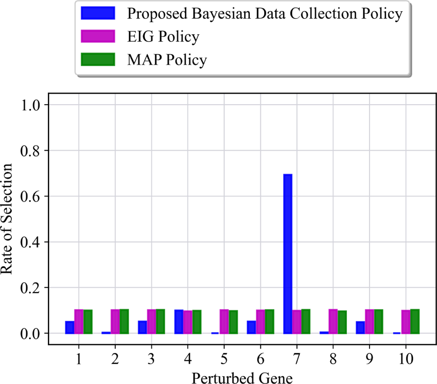
In the second part of our experiments, we considered a more challenging scenario with three +1 and two −1 unknown interactions as: $r_{83}=+1,r_{54}=+1,r_{35}=-1,r_{96}=+1$, and $r_{67}=-1$. Including −1 interactions makes the inference more challenging, primarily due to the attractor structure of GRNs, and the fact that most genes spend their time at rest (inactivated state) under no-perturbation. The proposed perturbation policy is trained over 5000 episodes, in this case. Figure 6 represents the average results of all methods. Similar to the previous case, the maximum posterior probability of models under no perturbation stays very small even with larger data. For the MAP and EIG perturbation policy, the average maximum posterior probability is smaller than the previous experiments. The reason for that is the existence of two −1 unknown interactions, which makes inferring the true topology more challenging. From Figure 6, one can see that the average maximum posterior probability is 0.5 after 50 perturbed data using MAP and EIG policies. In contrast, a much larger performance is achieved under the proposed perturbation policy. The average maximum posterior probability under the proposed policy is increased to 0.5 after about 5 perturbations (as opposed to 50 for the MAP and EIG perturbations) and larger than 0.95 after 9 perturbations. This demonstrates the capability of the proposed framework in systematically choosing the perturbation sequence and increasing the performance of the inference process. Moreover, Figure 8 represents the distribution of perturbations up to time step 20 for different perturbation policies. The perturbation over gene 7 is the most selected perturbation among the other genes. It is evident from Figures 5 and 8 that the perturbations may not always correspond directly to the genes associated with the unknown interactions. This observation arises due to the dynamic nature of regulatory networks, where a single perturbation can induce a network state that potentially leads to acquiring more informative data.

Fig. 6:

Action Distributions of Different Policies for Perturbation of Mammalian Cell Cycle Network with Five +1 Unknown Interactions.

Fig. 8:

Action Distributions of Different Policies for Perturbation of Mammalian Cell Cycle Network with Three +1 and Two −1 Unknown Interactions.

For the previous experiment, the average posterior probability of unknown interactions with respect to the number of data (i.e., number of perturbations) is visualized in Figure 7. The subplots in 5 columns correspond to five unknown interactions, and subplots in the first, second, and third rows are associated with our proposed perturbation policy, EIG perturbation policy, and no-perturbation case, respectively. Moreover, the posterior probability that unknown interactions are −1, 0, and +1 are indicated by black, blue, and red curves, respectively. Note that the MAP policy exhibits almost the same trend as the EIG policy for each of the interactions; thus, for better visualization, only the results for the EIG policy are shown in Figure 7. For instance, the subplot in the first row and fifth column represents the posterior probability of interaction $r_{67}(-1)$ under the proposed perturbation policy. In subplots of the first row, one can see that the average posterior probability of the true interaction has quickly approached 1. However, a much slower increase in the curves can be seen in the middle row subplots under the EIG perturbation policy. In particular, one can see that the average posterior probability of $r_{67}$ has the slowest increase relative to other interactions under the EIG perturbation policy. Finally, as it can be seen in the last row of the subplots, the average posterior probability for all interactions stays around $\frac{1}{3}$, similar to their prior probabilities. This indicates the poor performance of inference and difficulty of distinguishing between the true topology using the data from no-perturbation case.

Fig. 7:

Progress of Posterior Probability of Unknown Regulations $\left({\mu }_k\right)$ under Different Policies for Perturbation of Mammalian Cell Cycle Network with 5 Unknown Interactions.

Now, we examine the impact of perturbation space on the performance of the proposed method. We consider two cases: 1) 4-gene perturbation, which includes CycD, p27, CycE, and Cdh1 in perturbation space; 2) 7-gene perturbation, consisting of the CycD, p27, CycE, Cdh1, E2F, CycA, and Cdc20. Notice that in practice, the perturbation space is controlled by the availability of drugs for perturbing a specific set of genes. The process noise is set to be $p=0.001$ in this case. The proposed perturbation policy is trained using 6500 and 9000 episodes for 4-gene and 7-gene cases, respectively. The average performance of different perturbation policies in the case of 4-gene and 7-gene are shown in Figure 9. In both cases, the proposed perturbation policy outperforms the MAP, EIG, and no-perturbation policies. For the 4-gene case shown in Figure 9(a), one can see that the average maximum posterior probability under the proposed perturbation policy does not get to a high value as in the 10-gene perturbation case shown in Figure 6. In contrast, for the 7-gene case shown in Figure 9(b), the average maximum posterior probability is higher than the 4-gene case. This demonstrates the impact and importance of having extra three genes in the perturbation space to enable efficient data acquiring. It is noteworthy that the average maximum posterior probability in the 7-gene case falls below the 10-gene perturbation case in Figure 6, which again shows the advantage of having more control over the perturbations. More analyses regarding the perturbation spaces are included in the supplementary materials.

Fig. 9:

Performance Comparison of Different Policies for Perturbation of Mammalian Cell Cycle Network with 5 Unknown Interactions and (a) 4 Possible Perturbations Instead of 10, (b) 7 Possible Perturbations Instead of 10.

Next, the impact of large process noise on the performance of the proposed framework is analyzed. We considered the same set of 5 unknown interactions as our last experiment (i.e., $r_{83},r_{54},r_{35},r_{96}$ and $r_{67}$). Unlike the previous cases with small process noise $p=0.001$, we consider $p=0.1$ to account for a more stochastic/chaotic regulatory network. The training process in this case was more difficult and timeconsuming than previous cases, which can be explained by the need for propagation of the huge uncertainty during the learning process. The proposed perturbation policy is trained over 10,000 episodes in this case, which is much larger than the previous two scenarios with small process noise.

The average results for different policies are shown in Figure 10. It can be seen that the proposed method has the largest average maximum posterior probability in various numbers of data compared to the EIG, MAP, and no perturbation policies. Moreover, compared to previous cases, a slower increase in the average maximum posterior probability under the proposed perturbation policy is observed. The reason is that the system state is governed by the learned perturbation process as well as the noise process, where the large noise makes the planning more challenging. An interesting point in this scenario is the increase in the average maximum posterior probability under no-perturbed data. This is because the process noise, in this case, acts like random perturbations, which puts the system more often out of its attractor states, and helps to increase the performance of the inference process.

Fig. 10:

Performance Comparison of Different Policies for Perturbation of Mammalian Cell Cycle Network with 5 Unknown Interactions in Presence of High Process Noise.

Finally, Table II shows the accuracy of different perturbation policies in inferring the true regulatory network model during the perturbation process. Here, we report the exact rate of true inference rather than the average maximum posterior probability. In other words, a single model with the highest likelihood value is selected as ${\theta }_k^{\mathrm{M}\mathrm{A}\mathrm{P}}$ at any given time, and the rate of ${\theta }_k^{\mathrm{M}\mathrm{A}\mathrm{P}}$ matching with ${\theta }^{*}$ averaged over 1000 runs is reported. If multiple models hold the same maximum posterior probability, a random model is selected as the inferred model. The results for small and large noise conditions are shown in Table II. As expected, the performance of the perturbation process is lower under the high noise case. Meanwhile, One can see that the proposed method has the highest rate of true inference compared to other methods. As seen in the previous results, the larger performance difference can be seen in the presence of a smaller number of data. For example, in the low noise case, with only 10 steps, the true model has been accurately inferred 99.2% through perturbed data under the proposed policy compared to the inference rate of 34% under the MAP policy, 33.1% under the EIG policy, and 0% under no perturbation case.

TABLE II:

The Rate of True Inference under Different Perturbation Policies.

	p = 0.001 (Low Noise)					p = 0.1 (High Noise)
	10 Steps	20 Steps	30 Steps	40 Steps	50 Steps	10 Steps	20 Steps	30 Steps	40 Steps	50 Steps
Proposed Method	0.992	0.995	0.995	0.995	0.995	0.392	0.66	0.798	0.847	0.885
EIG Policy	0.331	0.632	0.818	0.909	0.959	0.241	0.496	0.646	0.739	0.805
MAP Policy	0.34	0.636	0.812	0.912	0.965	0.262	0.499	0.667	0.745	0.815
No Perturbation	0.0	0.001	0.003	0.004	0.004	0.166	0.401	0.546	0.669	0.727

C. Gut Microbial Community

In this part, we study the performance of our proposed method on the gut microbial community [37]. This microbial community plays a critical role in the normal intestinal functions. Mutation or damage to this community can lead to different serious illnesses such as obesity, diabetes, and even neurological disorders. The pathway diagram of the gut microbial community network is shown in Figure 11. The state vector consists of X_k = [Cli., Lachn., Lachn_other, Other, Barn., C_diff, Enterobact., Enteroco., Mol., Blautia]^T. The connectivity matrix and bias vector for the gut microbial network can be expressed using the pathway diagram in Figure 11 as:

$$\begin{gathered} R=\left[\begin{array}{cccccccccc}+1& -1& -1& -1& -1& 0& 0& 0& 0& 0\\ 0& +1& +1& +1& +1& 0& 0& 0& 0& 0\\ 0& +1& +1& +1& +1& 0& 0& 0& 0& 0\\ 0& +1& +1& +1& +1& 0& 0& 0& 0& 0\\ 0& 0& 0& 0& 0& -1& 0& 0& 0& 0\\ 0& 0& 0& 0& 0& +1& 0& +1& 0& 0\\ 0& 0& 0& 0& 0& 0& +1& +1& 0& 0\\ 0& 0& 0& 0& 0& 0& 0& 0& 0& +1\\ 0& 0& 0& 0& 0& 0& 0& +1& +1& 0\\ 0& 0& 0& 0& 0& 0& 0& +1& 0& +1\end{array}\right], \\ e={\left[\begin{array}{llllllllll}\frac{-1}{2}\hfill & \frac{-1}{2}\hfill & \frac{-1}{2}\hfill & \frac{-1}{2}\hfill & \frac{-1}{2}\hfill & \frac{-1}{2}\hfill & \frac{-1}{2}\hfill & \frac{-1}{2}\hfill & \frac{-1}{2}\hfill & \frac{-1}{2}\hfill \end{array}\right]}^T. \end{gathered}$$ (38)

Fig. 11:

Pathway Diagram for the Gut Microbial Community.

For our experiments, we consider the following 5 unknown interactions: $r_{23}=+1,r_{68}=+1,r_{108}=+1,r_{810}=+1,r_{41}=0$. The same set of parameters outlined in Table I are used here, and the system is assumed to be under 10-gene perturbation. The process noise is also set as $p=0.001$. In this scenario, the proposed perturbation policy is trained over 2500 episodes. Figure 12 shows the average results of different methods for perturbation. It can be seen that the proposed perturbation policy exceeds the performance of the other three policies in all the steps. We can also see poor inference performance under no-perturbed data and better inference results under the MAP and EIG perturbation policies. One can also see that the highest average maximum posterior probability of the MAP and EIG policies achieved after 50 perturbations is about 0.6, while this performance is achieved after about 8 perturbations under the proposed perturbation policy.

Fig. 12:

Performance Comparison of Different Policies for Perturbation of Gut Microbial Community Network with 5 Unknown Interactions.

VI. Conclusion

This paper developed a Bayesian lookahead perturbation policy for regulatory networks under uncertainty. We considered a general class of Boolean network models to represent regulatory networks. Assuming that a partial knowledge about the interactions between components of networks is available, we formulate the inference process through the maximum aposteriori (MAP) criterion. The perturbation process aims to flip the state value of targeted components at any given time to maximize the rate of MAP inference under the perturbed data. We optimally formulate the perturbation process in a reinforcement learning context and derive a scalable near-optimal Bayesian perturbation policy using deep reinforcement learning. The proposed method learns the perturbation policy offline (i.e., through planning) without the need for any real data. We demonstrated the high performance of the proposed policy through numerical experiments on two well-known regulatory network models: a mammalian cell cycle gene regulatory network, and a gut microbial community network.

Our future work will include scaling the proposed scheme to larger regulatory networks consisting of large and non-discrete parameters. We will further investigate problems with large and continuous perturbation spaces, which are common in applications such as inducing drugs. We will also study perturbations in complex regulatory networks and networks with partial state observability.

Biographies

Mohammad Alali is a third-year Ph.D. candidate in Electrical Engineering at Northeastern University. He received his B.Sc. degree in Electrical Engineering from University of Tehran, Tehran, Iran, in 2018, and M.Sc. degree in Electrical Engineering from Montana State University, Bozeman, USA, in 2021. His research interests lie in the domains of reinforcement learning, Bayesian statistics, machine learning, and experimental design. More specifically, he is currently investigating several projects with a focus on fast and efficient inference of various observable/ partially observable Markov models. He is the recipient of the Best Paper Finalist award from the American Control Conference in 2023.

Mahdi Imani received his Ph.D. degree in Electrical and Computer Engineering from Texas A&M University, College Station, TX in 2019. He is currently an Assistant Professor in the Department of Electrical and Computer Engineering at Northeastern University. His research interests include machine learning, Bayesian statistics, and decision theory, with a wide range of applications from computational biology to cyber-physical systems. He is the recipient of several awards, including the NIH NIBIB Trailblazer award in 2022, the Oracle Research Award in 2022, the NSF CISE Career Research Initiation Initiative award in 2020, the Association of Former Students Distinguished Graduate Student Award for Excellence in Research-Doctoral in 2019, and the Best Paper Finalist award from the American Control Conference in 2023 and the 49th Asilomar Conference on Signals, Systems, and Computers in 2015.

References

- [1].Davidson EH, The regulatory genome: gene regulatory networks in development and evolution. Elsevier, 2010. [Google Scholar]
- [2].Shmulevich I, Dougherty ER, and Zhang W, “From Boolean to probabilistic Boolean networks as models of genetic regulatory networks,” Proceedings of the IEEE, vol. 90, no. 11, pp. 1778–1792, 2002. [Google Scholar]
- [3].Li Y, Xiao J, Chen L, Huang X, Cheng Z, Han B, Zhang Q, and Wu C, “Rice functional genomics research: past decade and future,” Molecular plant, vol. 11, no. 3, pp. 359–380, 2018. [DOI] [PubMed] [Google Scholar]
- [4].Salama E-S, Govindwar SP, Khandare RV, Roh H-S, Jeon B-H, and Li X, “Can omics approaches improve microalgal biofuels under abiotic stress?,” Trends in plant science, 2019. [DOI] [PubMed] [Google Scholar]
- [5].Misra N, Panda PK, and Parida BK, “Agrigenomics for microalgal biofuel production: An overview of various bioinformatics resources and recent studies to link OMICS to bioenergy and bioeconomy,” Omics: a journal of integrative biology, vol. 17, no. 11, pp. 537–549, 2013. [DOI] [PMC free article] [PubMed] [Google Scholar]
- [6].Gordon JI, “Honor thy gut symbionts redux,” Science, vol. 336, no. 6086, pp. 1251–1253, 2012. [DOI] [PubMed] [Google Scholar]
- [7].Bergman E, “Energy contributions of volatile fatty acids from the gastrointestinal tract in various species,” Physiological reviews, vol. 70, no. 2, pp. 567–590, 1990. [DOI] [PubMed] [Google Scholar]
- [8].Rosenberg E, Sharon G, Atad I, and Zilber-Rosenberg I, “The evolution of animals and plants via symbiosis with microorganisms,” Environmental microbiology reports, vol. 2, no. 4, pp. 500–506, 2010. [DOI] [PubMed] [Google Scholar]
- [9].Ud-Dean SM and Gunawan R, “Optimal design of gene knockout experiments for gene regulatory network inference,” Bioinformatics, vol. 32, no. 6, pp. 875–883, 2015. [DOI] [PMC free article] [PubMed] [Google Scholar]
- [10].Logsdon BA and Mezey J, “Gene expression network reconstruction by convex feature selection when incorporating genetic perturbations,” PLoS computational biology, vol. 6, no. 12, p. e1001014, 2010. [DOI] [PMC free article] [PubMed] [Google Scholar]
- [11].Dong Z, Song T, and Yuan C, “Inference of gene regulatory networks from genetic perturbations with linear regression model,” PloS one, vol. 8, no. 12, p. e83263, 2013. [DOI] [PMC free article] [PubMed] [Google Scholar]
- [12].Cai X, Bazerque JA, and Giannakis GB, “Inference of gene regulatory networks with sparse structural equation models exploiting genetic perturbations,” PLoS computational biology, vol. 9, no. 5, p. e1003068, 2013. [DOI] [PMC free article] [PubMed] [Google Scholar]
- [13].Steinke F, Seeger M, and Tsuda K, “Experimental design for efficient identification of gene regulatory networks using sparse bayesian models,” BMC systems biology, vol. 1, no. 1, pp. 1–15, 2007. [DOI] [PMC free article] [PubMed] [Google Scholar]
- [14].Spieth C, Streichert F, Speer N, and Zell A, “Iteratively inferring gene regulatory networks with virtual knockout experiments,” in Workshops on Applications of Evolutionary Computation, pp. 104–112, Springer, 2004. [Google Scholar]
- [15].Ideker TE, Thorsson V, and Karp RM, “Discovery of regulatory interactions through perturbation: inference and experimental design,” in Pacific symposium on biocomputing, vol. 5, pp. 302–313, 2000. [DOI] [PubMed] [Google Scholar]
- [16].Akutsu T, Kuhara S, Maruyama O, and Miyano S, “Identification of genetic networks by strategic gene disruptions and gene overexpressions under a Boolean model,” Theoretical Computer Science, vol. 298, no. 1, pp. 235–251, 2003. [Google Scholar]
- [17].Imani M and Ghoreishi SF, “Optimal finite-horizon perturbation policy for inference of gene regulatory networks,” IEEE Intelligent Systems, 2020. [Google Scholar]
- [18].Shmulevich I and Dougherty ER, Probabilistic Boolean networks: the modeling and control of gene regulatory networks. SIAM, 2010. [Google Scholar]
- [19].Imani M, Dehghannasiri R, Braga-Neto UM, and Dougherty ER, “Sequential experimental design for optimal structural intervention in gene regulatory networks based on the mean objective cost of uncertainty,” Cancer informatics, vol. 17, 2018. [DOI] [PMC free article] [PubMed] [Google Scholar]
- [20].Ravari A, Ghoreishi SF, and Imani M, “Optimal recursive expert-enabled inference in regulatory networks,” IEEE Control Systems Letters, vol. 7, pp. 1027–1032, 2023. [DOI] [PMC free article] [PubMed] [Google Scholar]
- [21].Hosseini SH and Imani M, “Learning to fight against cell stimuli: A game theoretic perspective,” in IEEE Conference on Artificial Intelligence, 2023 [DOI] [PMC free article] [PubMed] [Google Scholar]
- [22].Ravari A, Ghoreishi S, and Imani M, “Structure-based inverse reinforcement learning for quantification of biological knowledge,” in IEEE Conference on Artificial Intelligence, 2023. [DOI] [PMC free article] [PubMed] [Google Scholar]
- [23].Imani M and Braga-Neto UM, “Maximum-likelihood adaptive filter for partially observed Boolean dynamical systems,” IEEE Transactions on Signal Processing, vol. 65, no. 2, pp. 359–371, 2017. [Google Scholar]
- [24].Imani M, Dougherty ER, and Braga-Neto U, “Boolean kalman filter and smoother under model uncertainty,” Automatica, vol. 111, 2020. [Google Scholar]
- [25].Mnih V, Kavukcuoglu K, Silver D, Rusu AA, Veness J, Bellemare MG, Graves A, Riedmiller M, Fidjeland AK, Ostrovski G, et al. , “Human-level control through deep reinforcement learning,” Nature, vol. 518, no. 7540, p. 529, 2015. [DOI] [PubMed] [Google Scholar]
- [26].Sutton RS and Barto AG, Reinforcement Learning: An Introduction. Cambridge, MA, USA: A Bradford Book, 2018. [Google Scholar]
- [27].Kingma DP and Ba J, “Adam: A method for stochastic optimization,” CoRR, vol. abs/1412.6980, 2015. [Google Scholar]
- [28].Lindley DV, “On a Measure of the Information Provided by an Experiment,” The Annals of Mathematical Statistics, vol. 27, no. 4, pp. 986 – 1005, 1956. [Google Scholar]
- [29].Tigas P, Annadani Y, Jesson A, Schölkopf B, Gal Y, and Bauer S, “Interventions, where and how? experimental design for causal models at scale,” in Advances in Neural Information Processing Systems, 2022. [Google Scholar]
- [30].Zemplenyi M and Miller JW, “Bayesian Optimal Experimental Design for Inferring Causal Structure,” Bayesian Analysis, pp. 1 – 28, 2022. [Google Scholar]
- [31].Linzner D and Koeppl H, “Active learning of continuous-time bayesian networks through interventions,” in Proceedings of the 38th International Conference on Machine Learning (M. Meila and T. Zhang, eds.), vol. 139 of Proceedings of Machine Learning Research, pp. 6692–6701, PMLR, 18–24 Jul 2021. [Google Scholar]
- [32].Tasiudi E, Lormeau C, Kaltenbach H-M, and Stelling J, “Designing genetic perturbation experiments for model selection under uncertainty,” IFAC-PapersOnLine, vol. 53, no. 2, pp. 15864–15869, 2020. 21st IFAC World Congress. [Google Scholar]
- [33].Foster A, Ivanova DR, Malik I, and Rainforth T, “Deep adaptive design: Amortizing sequential bayesian experimental design,” in Proceedings of the 38th International Conference on Machine Learning (M. Meila and T. Zhang, eds.), vol. 139 of Proceedings of Machine Learning Research, pp. 3384–3395, PMLR, 18–24 Jul 2021. [Google Scholar]
- [34].Blau T, Bonilla EV, Chades I, and Dezfouli A, “Optimizing sequential experimental design with deep reinforcement learning,” in Proceedings of the 39th International Conference on Machine Learning (K. Chaudhuri, S. Jegelka, L. Song, C. Szepesvari, G. Niu, and S. Sabato, eds.), vol. 162 of Proceedings of Machine Learning Research, pp. 2107–2128, PMLR, 17–23 Jul 2022. [Google Scholar]
- [35].Fauré A, Naldi A, Chaouiya C, and Thieffry D, “Dynamical analysis of a generic Boolean model for the control of the mammalian cell cycle,” Bioinformatics, vol. 22, no. 14, pp. e124–e131, 2006. [DOI] [PubMed] [Google Scholar]
- [36].Alali M and Imani M, “Inference of regulatory networks through temporally sparse data,” Frontiers in control engineering, vol. 3, p. 1017256, 2022. [DOI] [PMC free article] [PubMed] [Google Scholar]
- [37].Steinway SN, Biggs MB, Loughran TP, Papin JA Jr, and Albert R, “Inference of network dynamics and metabolic interactions in the gut microbiome,” PLOS Computational Biology, vol. 11, pp. 1–25, June 2015. [DOI] [PMC free article] [PubMed] [Google Scholar]
Associated Data
This section collects any data citations, data availability statements, or supplementary materials included in this article.