Predicting contrast sensitivity functions with digital twins

Abstract

We developed and validated digital twins (DTs) for contrast sensitivity function (CSF) across 12 prediction tasks using a data-driven, generative model approach based on a hierarchical Bayesian model (HBM). For each prediction task, we utilized the HBM to compute the joint distribution of CSF hyperparameters and parameters at the population, subject, and test levels. This computation was based on a combination of historical data (N = 56), any new data from additional subjects (N = 56), and “missing data” from unmeasured conditions. The posterior distributions of the parameters in the unmeasured conditions were used as input for the CSF generative model to generate predicted CSFs. In addition to their accuracy and precision, these predictions were evaluated for their potential as informative priors that enable generation of synthetic quantitative contrast sensitivity function (qCSF) data or rescore existing qCSF data. The DTs demonstrated high accuracy in group level predictions across all tasks and maintained accuracy at the individual subject level when new data were available, with accuracy comparable to and precision lower than the observed data. DT predictions could reduce the data collection burden by more than 50% in qCSF testing when using 25 trials. Although further research is necessary, this study demonstrates the potential of DTs in vision assessment. Predictions from DTs could improve the accuracy, precision, and efficiency of vision assessment and enable personalized medicine, offering more efficient and effective patient care solutions.

Introduction

The concept of a digital twin (DT) was introduced as an ideal framework for product life cycle management by Grieves in 2002¹, comprising three components: (1) a physical system, (2) a corresponding virtual model, and (3) twinning, which is a bidirectional data flow that provides physical-to-virtual (P2V) and virtual-to-physical (V2P) connections^2,3. The definition was broadened by the American Institute of Aeronautics and Astronautics: “A digital twin is a set of virtual information constructs that mimics the structure, context, and behavior of a natural, engineered, or social system (or system-of-systems), is dynamically updated with data from its physical twin, has a predictive capability, and informs decisions that realize value. The bidirectional interaction between the virtual and the physical is central to the digital twin.”^4,5. The Committee on Foundational Research Gaps and Future Directions for Digital Twins of the National Academies highlighted two central elements of the definition: “the phrase predictive capability to emphasize that a digital twin must be able to issue predictions beyond the available data to drive decisions that realize value,” and “the bidirectional interaction, which comprises feedback flows of information from the physical system to the virtual representation and from the virtual back to the physical system to enable decision making, either automatic or with humans in the loop.”⁶.

Since their inception, DTs have found numerous applications in fields where forecasts and predictions are crucial, including atmospheric and climate sciences, business, engineering, finance, and health care^6–13. Designed to provide timely and actionable information tailored to decision-making⁴, DTs simulate real world conditions, respond to changes, improve operations, and add value. According to McKinsey & Company, investments in DT will surpass $48 billion by 2026¹⁴.

In healthcare, DTs have found applications under the umbrella field of precision medicine². Proponents of precision medicine suggest that DTs can help identify individuals at-risk for disease, which provides the opportunity for early intervention to prevent worse outcomes. The prediction of treatment outcomes can also enable the development of personalized interventions optimized for each individual patient^15–20. In addition, both the US food and drug administration (FDA) and the European medicines agency (EMA) have issued guidelines for using DTs in randomized controlled trials (TwinRCTs) to mitigate risks in treatment development and streamline the evaluation of new technology. Specifically, DTs of patients in a treatment arm can be used as virtual patients in a control arm, which increases the effective number of patients through combination with real patients, and can enable faster and smaller trials by enhancing statistical power²¹. DTs have also been utilized for safety assessment in over 500 FDA submissions²².

The scale and modeling methods of DT depend on the nature of the physical system and the desired level of detail, fidelity, and functionality^3,11,13,23. In healthcare applications, DTs can span a broad spectrum of biological scales, encompassing molecular, subcellular, and cellular levels, as well as entire systems (e.g., digestive system), functions (e.g., vision), individual humans, populations, and the biosphere^2,19,22–27. They can also represent medical devices, such as the OCT machine, or healthcare organizations.

Various DT modeling methods have been developed to create sufficiently representative virtual replicas of physical entities, processes, or objects, including geometric modeling, physics-based modeling, data-driven modeling, physics-informed machine-learning modeling, and systems modeling²⁸. For example, Subramanian²⁹ created a DT of the liver in homeostasis to show improved phenotypes comparable to clinical trials. Fisher et al.³⁰ used existing longitudinal data in cognitive exams and labs from patients with Alzheimer’s disease to create DTs and generated synthetic patient data at different time points to simulate natural disease progression; the data generated by DTs were statistically indiscernible from real collected data.

In this proof-of-concept study, we employed a data-driven, generative model approach to develop DTs for the contrast sensitivity function (CSF), based on a group of human observers tested under different luminance conditions.

The CSF characterizes contrast sensitivity (1/threshold) as a function of spatial frequency. As a fundamental assay of spatial vision, it is closely related to daily visual activities in both normal and impaired vision^31–38. It has emerged as an important endpoint for staging eye diseases and assessing treatment efficacy^39–66. Importantly, the CSF varies not only with stimulus conditions such as retinal luminance⁶⁷, temporal frequency^68,69, and eccentricity^70,71, but also with disease progression and treatment^40–45. Predicting CSF for new observers or existing observers in not-yet measured conditions could help predict human performance in new conditions, identify potential risks and benefits of interventions, and enable personalized treatment for each individual patient. The predictions could also serve as informative priors to reduce test burdens in new measurements. Additionally, at the group level, the DTs of clinical study patients in an active arm have potential value as controls in TwinRCTs.

Previously, we developed a three-level Hierarchical Bayesian Model (HBM) to comprehensively model an entire CSF dataset within a single-factor (luminance), multi-condition (3 luminance conditions), and within-subject experiment design⁷². This model utilized trial-by-trial data and employed a log parabola CSF functional form with three parameters as the generative model at the test level, in addition to hyperparameters at the subject and population levels, incorporating between-and within-subject covariances as well as conditional dependencies across levels. The performance of the HBM was evaluated using an existing dataset⁷³ of 112 subjects tested with quantitative contrast sensitivity function (qCSF)⁷⁴ across three luminance conditions. By leveraging information across subjects and conditions to constrain the estimates, the HBM generated more precise estimates of the CSF parameters than the Bayesian inference procedure, which treated data for each subject and experimental condition separately. This increased precision improved signal detection (increased $d^{\mathrm{\prime }}$) for comparisons in Area Under the Log CSF (AULCSF) and CSF parameters between different experimental conditions at the test level for each subject, along with larger statistical differences across subjects. Importantly, the HBM also captured strong covariances within and between subjects and luminance conditions.

Here, we expanded the application of the HBM to generate DTs for a population of CSF observers (Fig. 1). The trial-by-trial responses from historical data (Fig. 1a), i.e., existing qCSF testing observers (N = 56), were used to train a three-level HBM (Fig. 1b)⁷². This model derives the joint posterior probability distribution of CSF hyperparameters and parameters at the population, subject and test levels across conditions (Fig. 1c). It incorporates conditional dependencies across the three levels to improve estimates of CSF parameters for each test. In the HBM, the population-level distribution of hyperparameters describes the probability of CSF parameters across all subjects. The subject-level distributions, which are conditionally dependent on the population-level hyperparameters, represent the probability of CSF parameters at the test level. These parameters determine trial-by-trial response probabilities in each CSF test using a log-parabola model with three parameters and a psychometric function. The generative model allows the DTs to combine the joint posterior distribution with newly acquired data to predict CSFs for new observers or for existing observers in unmeasured conditions (Fig. 1d). These predictions can also serve as informative priors for subsequent testing in those conditions (Fig. 1e).

Fig. 1.

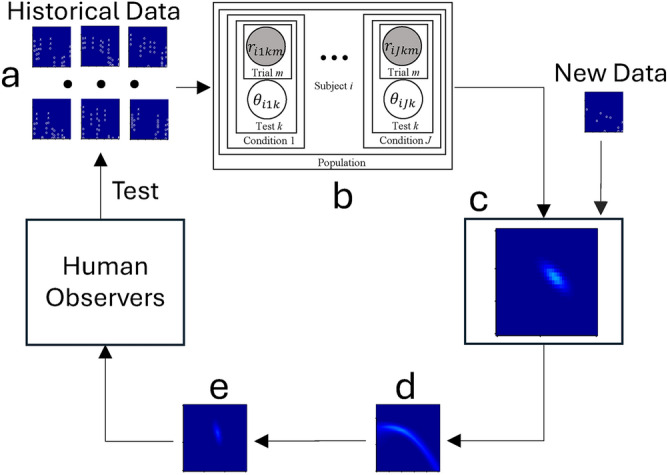
Digital twin for a population of CSF observers. The trial-by-trial responses from historical data (a), i.e., existing qCSF testing observers (N = 56), were used to train a three-level hierarchical Bayesian model (HBM; b) ⁷². This model derives the joint posterior probability distribution of CSF hyperparameters and parameters at the population, subject and test levels across conditions (c). It incorporates conditional dependencies across the three levels to improve estimates of CSF parameters for each test. The generative model allows the DTs to combine the joint posterior distribution with newly acquired data to predict CSFs for new observers or for existing observers in unmeasured conditions (d). These predictions can also serve as informative priors for subsequent testing in those conditions (e).

Our hypothesis is that the DTs created using the HBM can make accurate and relatively precise predictions of CSFs for new or existing observers in conditions where data is not available. To test this hypothesis, we conducted and assessed 12 prediction tasks (Table 1) using an existing CSF dataset involving 112 subjects tested in low-luminance (L), medium-luminance (M), and high-luminance (H) conditions⁷³. We divided the subjects into two groups. Group I’s data in all three luminance conditions served as historical data, while we aimed to predict CSFs for Group II subjects in the 12 prediction tasks (Table 1). In tasks 1 to 3, we utilized the DTs to predict CSFs for Group II subjects across all three conditions without incorporating new data, simulating scenarios for new observers who have not been previously tested. Subsequently, in tasks 4 to 9, we integrated Group II subjects’ CSF data from each luminance condition into the DTs to forecast their CSFs in the other two conditions. Tasks 10 to 12 involved predicting CSFs for Group II subjects in one of the three conditions by incorporating data from the other two conditions. These predictions were then compared against the actual observed data from Group II subjects in the corresponding conditions to evaluate the accuracy and reliability of the DTs.

Table 1.

Twelve prediction tasks.

Task	Training data from Group I	Training data from Group II	Group II predictions
1	L, M, H	None	L
2	L, M, H	None	M
3	L, M, H	None	H
4	L, M, H	L	M
5	L, M, H	L	H
6	L, M, H	M	L
7	L, M, H	M	H
8	L, M, H	H	L
9	L, M, H	H	M
10	L, M, H	L, M	H
11	L, M, H	L, H	M
12	L, M, H	M, H	L

In each prediction task, the dataset included historical data from Group I, any new data available from Group II, and “missing data” in the unmeasured conditions. The three-layer HBM⁷² was utilized to compute the joint distribution of the population-, subject- and test- level CSF hyperparameters and parameters from all the data in each prediction task (details in Supplementary Materials A). The posterior distributions of the parameters in the unmeasured conditions were utilized as input for the CSF generative model to generate predicted CSFs. Instead of applying the HBM solely to historical data and then integrating the resulting joint posterior distributions with new data to generate marginal distributions for predictions (Fig. 1), we directly incorporated historical data, new data, and “missing” data from unmeasured conditions into the HBM. By framing prediction tasks as a missing data problem within the model, we leveraged all available data sources in a unified manner. This approach not only enhances the accuracy and precision of predictions but also simplifies the computational process. The validation of the DTs involved assessing the accuracy and precision of their predictions by comparing them with the observed data. Additionally, the advantages of employing predictions from the DTs as informative priors in the qCSF test were evaluated.

Results

It took approximately 9 to18 hours and 120 MB RAM to compute the DT for a single prediction task in this study. The computation time varied with the amount of historical and new data. Here we present results based on the first 25 qCSF trials of the dataset because that is the typical number of trials used in clinical trials. Findings from 50 qCSF trials are generally consistent and reported in Supplementary Materials C.

Correlations in the historical data

Tables 2, 3, and 4 present correlation matrices from the historical data used to train the HBM. Supplementary Material B describes the posterior distributions of the CSF hyperparameters and parameters derived from the historical data (Group I) using the HBM.

Table 2.

Between-subject correlations of CSF hyperparameters at the population level.

		L			M			H
		PG	PF	BW	PG	PF	BW	PG	PF	BW
L	PG	1	−0.082	0.068	0.529	0.115	−0.101	0.398	0.000	0.082
	PF	−0.082	1	−0.808	0.244	0.363	−0.063	0.306	−0.004	0.156
	BW	0.068	−0.808	1	−0.197	−0.268	0.274	−0.209	0.044	−0.002
M	PG	0.529	0.244	−0.197	1	−0.139	0.022	0.523	0.012	0.035
	PF	0.115	0.363	−0.268	−0.139	1	−0.768	0.164	0.021	0.021
	BW	−0.101	−0.063	0.274	0.022	−0.768	1	−0.073	−0.014	0.222
H	PG	0.398	0.306	−0.209	0.523	0.164	−0.073	1	−0.448	0.364
	PF	0.000	−0.004	0.044	0.012	0.021	−0.014	−0.448	1	−0.860
	BW	0.082	0.156	−0.002	0.035	0.021	0.222	0.364	−0.860	1

PG: peak gain, PF: peak spatial frequency, BW: bandwidth.

Table 3.

Within-subject correlations of CSF hyperparameters at the subject level.

		L			M			H
		PG	PF	BW	PG	PF	BW	PG	PF	BW
L	PG	1	−0.482	0.195
	PF	−0.482	1	−0.885
	BW	0.195	−0.885	1
M	PG				1	−0.402	0.062
	PF				−0.402	1	−0.882
	BW				0.062	−0.882	1
H	PG							1	−0.501	0.222
	PF							−0.501	1	−0.904
	BW							0.222	−0.904	1

PG: peak gain, PF: peak spatial frequency, BW: bandwidth.

Table 4.

Correlations of CSF parameters at the test level.

		L			M			H
		PG	PF	BW	PG	PF	BW	PG	PF	BW
L	PG	1	−0.308	0.018
	PF	−0.308	1	−0.903
	BW	0.018	−0.903	1
M	PG				1	−0.202	−0.107
	PF				−0.202	1	−0.899
	BW				−0.107	−0.899	1
H	PG							1	−0.314	0.025
	PF							−0.314	1	−0.907
	BW							0.025	−0.907	1

PG: peak gain, PF: peak spatial frequency, BW: bandwidth.

At the population level, the HBM revealed strong positive correlations between peak gains (PG) across luminance conditions (0.398 to 0.529) and strong negative correlations between peak spatial frequency (PF) and bandwidth (BW) within each luminance condition (−0.860 to −0.768). Similarly, at the subject level, it identified strong negative correlations between PG and PF (−0.501 to −0.402) and strong negative correlations between PF and BW within each luminance condition (−0.904 to −0.882). Additionally, at the test level, the model found strong negative correlations between PF and BW within each luminance condition (−0.907 to −0.899).

These robust correlations indicate that CSF hyperparameters and parameters are highly correlated between- and within-subjects across conditions at all three levels of the hierarchy. They represent the fundamental mathematical properties utilized by the DTs to make predictions.

Individual subject level predictions

In this section, the results of the 12 prediction tasks at the individual subject level are presented. By utilizing the observed data from all subjects in Group II, a comparison was made between the predictions and the actual observed data. Generally, the alignment between predictions and observations improved as more new data became available for computing the predictions, resulting in increased accuracy and precision. For example, predictions for the L condition showed improvements from having no new data to having data in either the M or H condition, and further improvement with data in both the M and H conditions.

To quantify the similarity between observed and predicted CSF parameter distributions, a linear discriminant classifier was used. A p-value of 1.0 indicates complete alignment, while a p-value of 0.0 indicates complete separation. Accuracy was measured as the absolute difference between the observed and predicted areas under the log CSF (AULCSF), while precision was quantified as the standard deviations (SD) of the predicted AULCSFs.

The first column of Fig. 2 presents the observed posterior distribution of PG and PF, along with the observed posterior CSF distribution for a typical subject (#90) in the L condition with 25 qCSF trials. Columns 2 to 5 display the predicted parameter and CSF distributions under different scenarios: no new data, new data in the M, H, and both the M and H conditions, respectively.

Fig. 2.

Predictions for subject #90 in the L condition. Column 1: Posterior distribution of PG and PF (row 1) and the CSF (row 2) from the observed data. Columns 2–5: Predicted distributions of PG and PF (row 1) and CSF (row 2) with no new data (column 2), new data in the M (column 3), H (column 4), and both the M and H (column 5) conditions. Circles and crosses represent correct and incorrect trials from the qCSF test.

The p-values obtained from the linear discriminant analysis of the observed and predicted CSF parameter distributions were 0.15, 0.31, 0.26, and 0.33 for the four prediction results. These values indicate that the predicted CSF parameter distributions were not significantly different from the observed distributions.

Regarding accuracy, the absolute differences between the predicted and observed AULCSFs were 0.343, 0.098, 0.132, and 0.086 log₁₀ units, respectively. Considering that the SD of the observed AULCSF was 0.045 log₁₀ units, the predicted AULCSFs were not significantly different from the observed AULCSF when there were new data for the prediction. However, the SDs of the predicted AULCSFs were 0.186, 0.143, 0.122, and 0.117 log₁₀ units, respectively, indicating lower precision compared to the observed AULCSF.

The results for the prediction tasks in the M and H conditions were similar (Figures S5 and S6 in Supplementary Materials B). For instance, in the M condition, the p-values between the predicted and observed CSF parameter distributions were 0.15, 0.29, 0.50, and 0.39. The absolute differences between the predicted and observed AULCSFs were 0.224, 0.043, 0.039, and 0.008 log₁₀ units, while the SDs of the predicted AULCSFs were 0.141, 0.116, 0.099, and 0.098 log₁₀ units. In comparison, the SD of the observed AULCSF was 0.059 log₁₀ units.

Similarly, in the H condition, the p-values between the predicted and observed CSF parameter distributions were 0.15, 0.20, 0.28, and 0.28. The absolute differences between the predicted and observed AULCSFs were 0.196, 0.043, 0.022, and 0.000 log₁₀ units, while the SDs of the predicted AULCSFs were 0.150, 0.117, 0.125, and 0.117 log₁₀ units. In comparison, the SD of the observed AULCSF was 0.059 log₁₀ units.

Across all 12 prediction tasks for all 56 subjects in Group II, none of the predicted CSF parameter distributions were significantly different from the observed (α = 0.05, with Bonferroni correction). Figure 3 displays scatter plots of the predicted and observed AULCSFs for all subjects in the 12 prediction tasks with 25 qCSF trials.

Fig. 3.

Scatter plots of the predicted and observed AULCSFs with 25 qCSF trials. Row 1: The L condition with no new data (column 1), new data in the M (column 2), H (column 3), and both the M and H conditions (column 4). Row 2: The M condition with no new data (column 1), new data in the L (column 2), H (column 3), and both the L and H (column 4). Row 3: The H condition (row 3) with no new data (column 1), new data in the L (column 2), M (column 3), and both the L and M (column 4).

Table 5 present the average absolute differences between the predicted and observed AULCSFs and the average SDs of the predicted AULCSFs across all 56 subjects in the 12 prediction tasks, with standard error (SE) in parenthesis. The average absolute differences decreased with the amount of new data available, indicating improved accuracy. Consistent with results for subject #90, the predicted AULCSFs were not significantly different from the observed when any new data became available. Similarly, precision of the predicted AULCSFs also improved with the amount of new data available.

Table 5.

Average absolute difference (AD) and standard deviations (SD).

		Number of conditions in the new data
		0	1		2
AD	L	0.112 (0.010)	0.066 (0.007)	0.071 (0.007)	0.063 (0.007)
	M	0.108 (0.011)	0.070 (0.008)	0.066 (0.008)	0.060 (0.007)
	H	0.101 (0.010)	0.069 (0.006)	0.071 (0.008)	0.066 (0.006)
SD	L	0.186 (0.0003)	0.134 (0.0005)	0.122 (0.0004)	0.114 (0.0004)
	M	0.141 (0.0002)	0.101 (0.0006)	0.092 (0.0003)	0.085 (0.0004)
	H	0.153 (0.0003)	0.115 (0.0004)	0.118 (0.0004)	0.109 (0.0005)

The average SDs of the predicted AULCSFs ranged from 0.186 to 0.114, 0.141 to 0.085 and 0.153 to 0.109 log₁₀ units for the L, M, and H prediction tasks, respectively. In comparison, the average SDs of the observed AULCSFs were 0.056, 0.063, and 0.065 log₁₀ units in the three conditions. On average, the SDs of the predicted AULCSFs with data from 0, 1, and 2 luminance conditions were 2.6, 1.8, and 1.7 times those from the observed data (Wilcoxon Signed-Rank Test⁷⁵, all p < 0.01, with Bonferroni correction).

Group level predictions

The predicted parameter and CSF distributions in the 12 prediction tasks at the group level were constructed by averaging the corresponding distributions from all 56 subjects in Group II. Figure 4 displays the observed and predicted distributions of PG and PF, as well as the corresponding CSF distributions at the group level in the L condition. Similar patterns were observed in those in the M and H conditions and were displayed in Figures S7 and S8 in the Supplementary Materials B.

Fig. 4.

Group level predictions in the L condition with 25 qCSF trials. Column 1: Posterior distribution of PG and PF (row 1) and the CSF (row 2) from the observed data. Columns 2–5: Predicted distributions of PG and PF (row 1) and CSF (row 2) with no new data (column 2), new data in the M (column 3), H (column 4), and both the M and H (column 5) conditions.

None of the predicted CSF parameter distributions at the group level were significantly different from the observed (all p > 0.05). Table 6 present the absolute differences between the predicted and observed AULCSFs and SDs of the predicted AULCSFs at the group level. Both the accuracy and precision of the predicted AULCSFs improved with the amount of new data available. The absolute difference between the predicted and observed AULCSFs ranged from 0.000 to 0.061 log₁₀ units, suggesting that the predicted AULCSFs were very close to the observed. The SDs of the predicted AULCSFs ranged from 0.019 to 0.039 log₁₀ units. In comparison, the SDs of the observed AULCSFs were 0.009, 0.010, and 0.011 log₁₀ units in the L, M, and H conditions. On average, the SDs of the predicted AULCSFs with new data from 0, 1, and 2 luminance conditions were 3.2, 2.4, and 2.2 times of the SDs of the observed AULCSFs. This suggests that while they were quite accurate, the predicted AULCSFs exhibited greater variabilities compared to the observed data.

Table 6.

Absolute differences (AD) and standard deviations (SD) at the group level.

		Number of conditions in the new data
		0	1		2
AD	L	0.042	0.000	0.042	0.036
	M	0.061	0.033	0.026	0.023
	H	0.031	0.020	0.000	0.017
SD	L	0.039	0.028	0.026	0.025
	M	0.028	0.022	0.021	0.019
	H	0.029	0.023	0.024	0.022

Using predicted parameter distributions as informative priors

We evaluated the benefits of using the predicted parameter distributions in the 12 prediction tasks as informative priors in the qCSF procedure. First, we used the informative priors to rescore existing data collected with an un-informative prior and evaluated the number of trials necessary to achieve comparable precision and statistically equivalent AULCSFs obtained with 25 qCSF trials. Because the stimulus sequences were not optimized with the informative priors in the existing dataset, we additionally used the informative priors in a simulated qCSF procedure to further evaluate the number of trials that can be saved when they were incorporated into the qCSF procedure directly.

Figure 5 shows the average absolute difference between the rescored and observed AULCSFs across all the 56 subjects in Group II as functions of the number of qCSF trials used in rescoring, as well as the average SD of the rescored AULCSFs. Both the average absolute differences and SDs decreased with the number of trials used in rescoring.

Fig. 5.

Average absolute difference between the rescored and observed AULCSF (orange solid lines) across all the 56 subjects in Group II as functions of the number of qCSF trials used in rescoring and average SD of the rescored AULCSFs (blue solid lines) are shown. In row 1, results in L condition are displayed with no new data (column 1), new data in the M (column 2), H (column 3), and both the M and H conditions (column 4). Row 2 shows results in the M condition with no new data (column 1), new data in the L (column 2), H (column 3), and both the L and H conditions (column 4). In row 3, results in the H condition are presented with no new data (column 1), new data in the L (column 2), M (column 3), and both the L and M conditions (column 4). The black dashed lines represent the average SDs of the observed AULCSFs with SD (grey shaded area), and error bars indicate standard errors.

Figure 6 depicts histograms of the number of trials needed in rescoring to reach statistically equivalent precision as the observed AUCLSFs. On average, 12.3 $\pm$ 0.1 trials were necessary. We also determined the number of trials needed to obtain estimated AULCSFs that are not significantly different from the observed and found that 8.9 $\pm$ 0.5 trials on average were required. Combining these results together, we conclude that the informative priors, even without trial-by-trial optimal stimulus selection, can save about 12.7 trials or 51% of the data collection burden in qCSF.

Fig. 6.

Histograms of the number of trials needed to reach comparable precision as the observed AUCLSFs in rescoring. Row 1: results in the L condition with no new data (column 1), new data in the M (column 2), H (column 3), and both the M and H (column 4) conditions. Row 2: results in the M condition with no new data (column 1), new data in the L (column 2), H (column 3), and both the L and H (column 4) conditions. Row 3: results in the H condition with no new data (column 1), new data in the L (column 2), M (column 3), and both the L and M (column 4) conditions. The average number of trials with standard error are displayed in each condition.

Next, we present results from the simulated qCSF experiment. In this simulation, we incorporated informative priors into the data collection process. Each simulation began with the predicted CSF parameter distribution as the informative prior. In the first trial, the qCSF algorithm selected the optimal test stimulus based on this prior. The simulated observer’s response was generated using the CSF parameters of the observer in the same condition and used to update the posterior CSF parameter distribution using Bayes’ rule. This updated posterior then served as the prior in the next trial. The process was repeated until we collected 25 trials.

We stimulated the qCSF test for all the 56 subjects in Group II with the informative priors from the 12 prediction tasks. Figure 7 illustrates the progression of the simulation, showing the average absolute difference between the AULCSFs obtained from the simulation and the observed data, along with the average SD of the simulated AULCSFs across all subjects. Both measures consistently decreased as the number of trials increased.

Fig. 7.

Average absolute difference between the AULCSFs from the simulated and observed data (orange solid lines) across all the 56 subjects in Group II as functions of the number of qCSF trials used in the simulation and average SDs of the simulated AULCSFs (blue solid lines) are shown. In row 1, results in the L condition are displayed with no new data (column 1), new data in the M (column 2), H (column 3), and both the M and H conditions (column 4). Row 2 shows results in the M condition with no new data (column 1), new data in the L (column 2), H (column 3), and both the L and H conditions (column 4). In row 3, results in the H condition are presented with no new data (column 1), new data in the L (column 2), M (column 3), and both the L and M conditions (column 4). The black dashed lines represent the average SDs of the observed AULCSFs with SD (grey shade area), and error bars indicate standard errors.

Moreover, Fig. 8 provides a histogram depicting the distribution of the number of trials needed to achieve statistically equivalent precision as the observed AULCSFs. On average, only 11.0 ± 0.2 trials were necessary. We also determined the number of trials needed to obtain estimated AULCSFs that are not significantly different from the observed and found that 8.8 $\pm$ 0.5 trials on average were required. Combining these results together, we conclude that the informative priors, can save about 14.0 trials or 56% of the data collection burden in qCSF.

Fig. 8.

Histograms of the number of trials needed to reach comparable precision as the observed AUCLSFs in the simulation experiment. Row 1: results in the L condition with no new data (column 1), new data in the M (column 2), H (column 3), and both the M and H (column 4) conditions. Row 2: results in the M condition with no new data (column 1), new data in the L (column 2), H (column 3), and both the L and H (column 4) conditions. Row 3: results in the H condition with no new data (column 1), new data in the L (column 2), M (column 3), and both the L and M (column 4) conditions. The average number of trials with standard error are displayed in each condition.

Discussion

In this proof-of-concept study, DTs were developed and validated for a population of CSF observers using a data-driven, generative model approach based on a three-level HBM. This HBM captured both between- and within-subject covariances between CSF hyperparameters and parameters across multiple conditions at all three levels of the hierarchy, providing fundamental mathematical properties used by the DTs to make CSF predictions for new or existing observers in unmeasured conditions.

The DTs demonstrated high accuracy in group level predictions across all tasks and maintained accuracy at the individual subject level when new data were available. Specifically, the absolute difference between the predicted and observed AULCSF estimates was comparable to the SD of the observed data, indicating reliable performance. However, the precision of the predictions was lower than that of the observed data. When used as informative priors to rescore existing qCSF data and simulate new qCSF tests, the DT predictions could reduce the data collection burden in qCSF testing by more than 50%, when using 25 trials, which are typically used in clinical settings. Additionally, the new test results could update the HBM in the DTs, establishing a real-time feedback loop between human observers and their DTs.

The accuracy and precision of DT predictions are significantly influenced by the quantity and quality of both historical and new subject data. In this study, the historical dataset included 56 subjects tested under three luminance conditions, which is relatively small compared to most clinical trials in this field. We observed that increasing the number of trials within each test in the historical data enhanced both the accuracy and precision of DT predictions. Specifically, using 50 qCSF trials from the same 56 subjects, the accuracy improved by 4%, 22%, and 25%, while precision increased by 2%, 9%, and 10%, compared to using only 25 qCSF trials. These improvements were observed in scenarios with no new data, new data in one condition, and new data in two conditions, respectively. Additionally, both accuracy and precision of DT predictions were positively correlated with the amount of new data available. For instance, with 25 qCSF trials in the historical data, accuracy increased by 36% and 41%, and precision improved by 29% and 36% with new data in one and two conditions, respectively, compared to the predictions without new data. With 50 trials per condition in the historical data, accuracy improved by 48% and 54%, and precision increased by 34% and 41%, in the presence of new data in one and two conditions, respectively. We also explored the effect of historical data sample size on DT predictions. When the historical dataset was reduced to 28 randomly selected subjects from Group I, each tested with 25 qCSF trials across the three luminance conditions, we recalculated the DT predictions for the 12 prediction tasks (see Table 1). Compared to predictions using the full set of 56 subjects with 25 qCSF trials each (Table 5), reducing the sample size resulted in a decrease in accuracy by 27%, 12%, and 9%, and a decrease in precision by 20%, 23%, and 23%, for scenarios with no new data, new data in one condition, and new data in two conditions, respectively (Table 7). These results highlight that a sufficient sample size is crucial for developing effective DTs for CSF, as inadequate data can significantly impair prediction performance.

Table 7.

Average AD and SD with 28 subjects in the historical dataset.

		Number of conditions in the new data
		0	1		2
AD	L	0.134 (0.011)	0.067 (0.007)	0.070 (0.007)	0.062 (0.007)
	M	0.138 (0.012)	0.085 (0.008)	0.082 (0.009)	0.073 (0.008)
	H	0.135 (0.012)	0.072 (0.007)	0.086 (0.009)	0.070 (0.007)
SD	L	0.218 (0.0003)	0.156 (0.0005)	0.144(0.0009)	0.132 (0.0009)
	M	0.160 (0.0003)	0.118 (0.0006)	0.108 (0.0004)	0.100 (0.0004)
	H	0.196 (0.0005)	0.157 (0.0008)	0.155 (0.0006)	0.145 (0.0007)

While individual components such as HBM, DTs, and Bayesian methods are well-established, this study introduces several key innovations: (1) the development and application of HBM-based DTs within the functional vision domain, (2) the novel approach of treating prediction tasks as missing data problems within the HBM framework, and (3) the incorporation of DT predictions as informative priors in qCSF testing. Although our implementation and validation of DTs were confined to CSF in a single normal vision population under three specific luminance conditions—limiting the generalizability of our findings to other populations, conditions, or eye diseases—the technical advancements promise significant potential for further exploration and broader applications. These include TwinRCT^21,22, precision medicine^19,76,77, and patient care^2,19,25. For instance, if we consider the M condition as the baseline, and the H and L conditions as the treatment and control arms in a randomized controlled trial, our prediction task 12 effectively emulates a TwinRCT. In this setup, DT predictions for the 56 Group II subjects in the L condition (control arm) were derived from their baseline (M) and treatment (H) data. Despite a lower precision in quantifying these virtual patients, their inclusion can still notably increase the effective sample size in the control arm, thereby enhancing the statistical power of the TwinRCT.

If we regard data in the L condition as the test results of an initial visit and the CSFs in the M and H condition as the treatment outcomes at two subsequent visits, our prediction tasks 4 and 5 emulate treatment predictions at different time points. This initial prediction can help clinicians choose the initial treatment plan. After the treatment starts and with the measurement at the follow-up visit, the conceptual equivalent to the M condition data in this study, the prediction for the H condition from the DTs of subjects with data in both the L and M conditions (task 10 in Table 1) can evaluate the effectiveness of the current treatment plan and help determine if any changes in the treatment are necessary.

Additionally, the DT predictions can serve as informative priors in adaptive testing for returning patients at their follow-up visits, reducing testing burden and improving patient care while reducing financial costs. The probabilistic predictions from the DT can 'close-the-loop’ in adaptive testing, acting as priors that further enhance test efficiencies and significantly decrease testing burden. Previously, we developed the hierarchical adaptive design optimization (HADO) framework to improve test efficiency with informative priors for new patients based on their disease categories^78,79. While HADO uses new patients’ disease categories to improve test efficiency with informative prior tailored to specific diseases, the current HBM leverages the within-patient covariance across conditions. The combination of the two leads to informative priors based on both group membership (e.g., diseases) and within-subject relationships across modalities, conditions, and timepoints in one HBM-based DT. Therefore, although we demonstrated DTs in a single normal vision population under three specific luminance conditions, to account for variations across different diseases and populations, DTs can be integrated with HADO.

The informative priors generated by DTs without any new data (tasks 1 to 3 in Table 1) for the to-be-measured subjects in our study utilize only the between-subject relationship and are the same for all patients with the same group membership. In contrast, the informative priors by DTs with data from one (tasks 4 to 9 in Table 1) and two (tasks 10 to 12 in Table 1) conditions use both between- and within-subject relationships and are individualized for each subject and test at each time point. Since we have demonstrated that the performance of informative priors increases with the amount of data available for the to-be-measured subjects, the DT can enhance HADO by incorporating within-subject information in addition to the between-subject relationship.

Furthermore, the bidirectional information flow between real patients and their DTs enables better sequential testing over time, as predictions from DTs based on previous testing serve as informative priors for current tests, resulting in higher accuracy, precision, and efficiency. While the qCSF uses only weakly informative priors and HADO uses the same informative prior for all patients with the same group membership, the DT offers a blueprint for personalized adaptive testing.

The DTs developed in this study are based on the hierarchical Bayesian modeling framework. Although only one test modality in three luminance conditions in a single normal vision population was modeled in this study, we have previously developed hierarchical Bayesian joint models (HBJM)⁸⁰ to model data from multiple test modalities, including functional vision tests such as visual acuity, CSF, and perimetry, and structural vision tests such as optical coherence tomography (OCT)⁸¹, fundus imaging, across different patient populations and different stages of diseases over multiple time points. The key in the current development is the quantification of the between- and within-subject/condition relationships with covariance hyperparameters at the population and subject levels with the HBM. With the HBJM, the DTs can be extended to incorporate both functional and structural vision assessments to further improve the accuracy and precision of disease staging and predictions for treatment outcomes of individual patients in precision medicine. Furthermore, DTs can also be developed to quantify relationships between multiple assessments over time with additional covariances and thus make predictions for disease progression or treatment outcome.

The DTs in this study cannot make prediction outside the scope of the existing data because the HBM only captures relationships among CSF parameters within the historical dataset. To extend predictions to new conditions, there are two main approaches: (1) expanding the historical data to include a broader range of conditions, (2) replacing the covariance matrix in the HBM with a function or process (e.g., Gaussian Process⁸²) that models the covariance as a function of conditions or time. In most practical applications of DTs in vision assessment, expanding the data is essential for establishing credibility and confidence. Even if the second approach is considered, the covariance matrix in the HBM remains crucial for identifying the appropriate functional form, particularly since we often lack prior knowledge of suitable functional forms.

We have developed and validated a two-step approach in an orientation identification perceptual learning study^83,84. In the first step⁸³, we used a non-parametric HBM to estimate thresholds every ten trials, enhancing the temporal resolution of the estimated learning curving, which typically derived from threshold estimates based on many trials. This finer temporal resolution enabled identification of a functional form with three component processes in addition to general learning: between-session forgetting, and rapid relearning and adaptation within sessions. In the second step⁸⁴, we developed a parametric HBM using the multi-component functional form identified in the first step. This model estimates the trial-by-trial learning curve and can predict thresholds for any trial, even those outside the historical data scope.

We chose the HBM for constructing the generative model of trial-by-trial CSF data in the DT because it incorporates a well-established functional form of the CSF^74,85. Instead of using machine learning to re-learn the optimal functional form for the CSF from the trial-by-trial data, we utilized a functional form based on domain-specific expertise developed through decades of research⁸⁶. This approach is advantageous because it leverages well-established knowledge rather than relying solely on artificial intelligence to determine the functional form. In addition, traditional statistical models in this domain are based on point estimate of CSF parameters. They do not use all the information in the trial-by-trial data to generate posterior probability distribution that are essential in the predictions of CSF with estimated uncertainty in unmeasured conditions.

On the Dell computer with an Intel Xeon W-2145 @ 3.70 GHz CPU (8 cores and 16 threads) and 64 GB of installed memory (RAM), it took approximately 9 to 18 h and 120 MB RAM to compute the DT for a single prediction task in this study. Although 18 h is still within practical time limits, scaling up the DTs to include more historical data, additional conditions, more new data, or more predictions may require more efficient computation methods. We are exploring pre-computed likelihood functions⁸⁷, Gaussian Process modeling⁸², and newly developed parallel MCMC algorithms to address this⁸⁸.

In conclusion, this study introduces DTs developed through a hierarchical Bayesian modeling approach for predicting the CSF . The DTs accurately predict CSF patterns, reducing testing burden and facilitating treatment evaluation in precision medicine. They emulate TwinRCTs, enhancing sample size and statistical power, and aid in treatment predictions over time. Additionally, DTs serve as informative priors in adaptive testing, improving patient care by incorporating both between- and within-subject relationships. The scalability of DTs extends beyond CSF, offering personalized disease staging and treatment outcome predictions. While effective for CSF data, alternative machine learning technologies may be needed for projections beyond existing data. Although further research is necessary, this study demonstrate the potential of DTs in vision assessment. Reliable predictions from DTs could improve the accuracy, precision, and efficiency of vision assessment and enable personalized medicine, offering more efficient and effective patient care solutions.

Methods

Data

The dataset used in this study comprised 112 college-aged subjects with normal or corrected-to-normal vision. They were tested with qCSF under low (2.62 cd/m²), medium (20.4 cd/m²), and high (95.4 cd/m²) background luminance conditions⁷³. Each trial presented three filtered letters of the same size, randomly sampled with replacement from 10 SLOAN letters (C, D, H, K, N, O, R, S, V, and Z), with the center spatial frequency and contrasts of the letters determined by the qCSF algorithm^73,74. A total of 50 trials were conducted under each luminance conditions. Subjects were required to verbally report the identities of the letters displayed on the screen. Written consent was obtained from all participants, and the study protocol adhered to the principles outlined in the Declaration of Helsinki, approved by the Institutional Review Board of human subject research of the Ohio State University.

Apparatus

All analysis was conducted on a Dell computer with Intel Xeon W-2145 @ 3.70 GHz CPU (8 cores and 16 threads) and 64 GB installed memory (RAM). The HBM was implemented in JAGS⁸⁹ in R⁹⁰.

Data analytics procedures

Supplementary Materials A provides detailed descriptions of the DTs, including their HBM core, evaluation procedures for the DT predictions, and methods for incorporating DT predictions as informative priors in qCSF testing. It also outlines procedures for quantifying the accuracy and precision of DT predictions and using them as informative priors to rescore existing data and simulate the qCSF procedure.

In the HBM, the priors for the mean of the CSF hyperparameters at the population level are uniform distributions covering the same range of CSF parameters used in the qCSF test, which has been effectively applied across various clinical populations^{46,47,51,53,55,56,59,62,91–93}. We employed the Bayesian inference procedure (BIP) to estimate the posterior distribution of CSF parameter for each test independently.

The weakly informative prior distribution of the covariance at the population level in the HBM was defined by a $9\times 9$ precision matrix with a Wishart distribution, degrees of freedom of 9, and an expected mean based on the covariance of estimated CSF parameters across all subjects and conditions from the BIP. For the subject-level covariance in each condition, the prior was defined by a $3\times 3$ precision matrix with a Wishart distribution, degrees of freedom of 3, and an expected mean based on the average covariance of the posterior distribution of the estimated CSF parameters across all subjects in that condition from the BIP. These weakly informative priors are critical for the HBM to converge within practical time limits.

In our previous study⁷², using these weakly informative covariance priors, the HBM took 54 h to converge and generate 10,000 effective samples. In contrast, using a diagonal covariance prior resulted in a 18% increase in computational time (63.5 h) to generate the same number of effective samples. Our findings align with other studies on the impact of priors on covariance estimation^94,95.

Author contributions

Dr. Zhao analyzed the data, wrote the manuscript, and prepared the figures. Dr. Lu designed the experiment, analyzed the data, and wrote the manuscript. All authors reviewed the manuscript.

Data availability

The datasets analyzed during the current study are available from the corresponding author upon reasonable request.

Declarations

Competing interests

Dr. Lesmes and Dr. Dorr have intellectual and equity interests, and hold employment in Adaptive Sensory Technology, Inc. (San Diego, CA). Dr. Lu has intellectual and equity interests in Adaptive Sensory Technology, Inc. (San Diego, CA) and Jiangsu Juehua Medical Technology, LTD (Jiangsu, China).

Supplementary Information

The online version contains supplementary material available at 10.1038/s41598-024-73859-x.

References

- 1.Grieves, M. & Vickers, J. Digital twin: mitigating unpredictable, undesirable emergent behavior in complex systems. In Transdisciplinary Perspectives on Complex Systems: New Findings and Approaches (eds Kahlen, F. J. et al.) (Springer International Publishing, 2017). [Google Scholar]
- 2.Xames, M. D. D. & Topcu, T. G. A Systematic Literature Review of Digital Twin Research for Healthcare Systems: Research Trends, Gaps, and Realization Challenges (IEEE Access, 2024). [Google Scholar]
- 3.Kritzinger, W., Karner, M., Traar, G., Henjes, J. & Sihn, W. Digital twin in manufacturing: A categorical literature review and classification. IFAC Pap. 51(11), 1016–1022. 10.1016/j.ifacol.2018.08.474 (2018). [Google Scholar]
- 4.Kobryn, P. A. The digital twin concept. Bridge 49(4), 16–20 (2019). [Google Scholar]
- 5.Glaessgen EH, Stargel DS. The Digital Twin Paradigm for Future NASA and U.S. Air Force Vehicles. (accessed March 27 2024) https://ntrs.nasa.gov/citations/20120008178
- 6.National Academies of Sciences Engineering and Medicine. Foundational Research Gaps and Future Directions for Digital Twins (The National Academies Press, 2023). [PubMed] [Google Scholar]
- 7.Abbott, D. Applied Predictive Analytics: Principles and Techniques for the Professional Data Analyst (John Wiley & Sons, 2014). [Google Scholar]
- 8.Eckerson, W. W. Predictive analytics. Ext. Value Your Data Warehous Invest. TDWI Best Pract. Rep. 1, 1–36 (2007). [Google Scholar]
- 9.Larose, D. T. Data Mining and Predictive Analytics (John Wiley & Sons, 2015). [Google Scholar]
- 10.Shmueli, G. & Koppius, O. R. Predictive analytics in information systems research. MIS Q. 35, 553–572 (2011). [Google Scholar]
- 11.Rasheed, A., San, O. & Kvamsdal, T. Digital twin: values, challenges and enablers from a modeling perspective. IEEE Access 8, 21980–22012. 10.1109/ACCESS.2020.2970143 (2020). [Google Scholar]
- 12.Liu, M., Fang, S., Dong, H. & Xu, C. Review of digital twin about concepts, technologies, and industrial applications. J. Manuf. Syst. 58, 346–361. 10.1016/j.jmsy.2020.06.017 (2021). [Google Scholar]
- 13.Semeraro, C., Lezoche, M., Panetto, H. & Dassisti, M. Digital twin paradigm: A systematic literature review. Comput. Ind. 130, 103469. 10.1016/j.compind.2021.103469 (2021). [Google Scholar]
- 14.McKinsey & Company. What is digital-twin technology? (accessed 21 March 2024); https://www.mckinsey.com/featured-insights/mckinsey-explainers/what-is-digital-twin-technology
- 15.Miner, G. D. et al.Practical Predictive Analytics and Decisioning Systems for Medicine: Informatics Accuracy and Cost-Effectiveness for Healthcare Administration and Delivery Including Medical Research (Academic Press, 2014). [Google Scholar]
- 16.Parikh, R. B., Obermeyer, Z. & Navathe, A. S. Regulation of predictive analytics in medicine. Science 363(6429), 810–812 (2019). [DOI] [PMC free article] [PubMed] [Google Scholar]
- 17.Peterson, E. D. Machine learning, predictive analytics, and clinical practice: can the past inform the present?. JAMA 322(23), 2283–2284 (2019). [DOI] [PubMed] [Google Scholar]
- 18.Zhang, Z., Zhao, Y., Canes, A., Steinberg, D. & Lyashevska, O. Predictive analytics with gradient boosting in clinical medicine. Ann. Transl. Med. 7(7), 152 (2019). [DOI] [PMC free article] [PubMed] [Google Scholar]
- 19.Kamel Boulos, M. N. & Zhang, P. Digital twins: From personalised medicine to precision public health. J. Pers. Med. 11(8), 745. 10.3390/jpm11080745 (2021). [DOI] [PMC free article] [PubMed] [Google Scholar]
- 20.Bruynseels, K., Santoni de Sio, F. & van den Hoven, J. Digital twins in health care: Ethical implications of an emerging engineering paradigm. Front. Genet.10.3389/fgene.2018.00031 (2018). [DOI] [PMC free article] [PubMed] [Google Scholar]
- 21.Lee, C. S. & Lee, A. Y. How artificial intelligence can transform randomized controlled trials. Transl. Vis. Sci. Technol. 9(2), 9–9. 10.1167/tvst.9.2.9 (2020). [DOI] [PMC free article] [PubMed] [Google Scholar]
- 22.National Academies of Sciences Engineering and Medicine (2023) Opportunities and Challenges for Digital Twins in Biomedical Research: Proceedings of a Workshop—in Brief. (The National Academies Press, Washington) [PubMed]
- 23.Wang, B. et al. Human digital twin in the context of industry 50. Robot. Comput. Integr. Manuf. 85, 102626. 10.1016/j.rcim.2023.102626 (2024). [Google Scholar]
- 24.Baker, G. H. & Davis, M. Digital twin in cardiovascular medicine and surgery. In Intelligence-Based Cardiology and Cardiac Surgery. Intelligence-Based Medicine: Subspecialty Series (eds Chang, A. C. & Limon, A.) (Academic Press, 2024). [Google Scholar]
- 25.Venkatesh, K. P., Brito, G. & Boulos, M. N. K. Health digital twins in life science and health care innovation. Annu. Rev. Pharmacol. Toxicol. 64, 159–170. 10.1146/annurev-pharmtox-022123-022046 (2024). [DOI] [PubMed] [Google Scholar]
- 26.Mahmoud Abdelhaleem Ali, A. & Mansour Alrobaian, M. Strengths and weaknesses of current and future prospects of artificial intelligence-mounted technologies applied in the development of pharmaceutical products and services. Saudi Pharm. J. 32, 102043. 10.1016/j.jsps.2024.102043 (2024). [DOI] [PMC free article] [PubMed] [Google Scholar]
- 27.Shengli, W. Is human digital twin possible?. Comput. Methods Programs Biomed. Update 1, 100014. 10.1016/j.cmpbup.2021.100014 (2021). [Google Scholar]
- 28.Thelen, A. et al. A comprehensive review of digital twin—Part 1: modeling and twinning enabling technologies. Struct. Multidiscip. Optim. 65(12), 354. 10.1007/s00158-022-03425-4 (2022). [Google Scholar]
- 29.Subramanian, K. Digital twin for drug discovery and development—The virtual liver. J. Indian Inst. Sci. 100(4), 653–662. 10.1007/s41745-020-00185-2 (2020). [Google Scholar]
- 30.Fisher, C. K., Smith, A. M. & Walsh, J. R. Machine learning for comprehensive forecasting of Alzheimer’s disease progression. Sci. Rep. 9(1), 13622. 10.1038/s41598-019-49656-2 (2019). [DOI] [PMC free article] [PubMed] [Google Scholar]
- 31.Arden, G. Importance of measuring contrast sensitivity in cases of visual disturbance. Br. J. Ophthalmol. 62(4), 198–209. 10.1136/bjo.62.4.198 (1978). [DOI] [PMC free article] [PubMed] [Google Scholar]
- 32.Ginsburg, A. P. Spatial filtering and vision: Implications for normal and abnormal vision. In Clinical Applications of Visual Psychophysics (eds Proenz, L. et al.) (Cambridge University Press, 1981). [Google Scholar]
- 33.Ginsburg, A. P. Contrast sensitivity and functional vision. Int. Ophthalmol. Clin. 43(2), 5–15 (2003). [DOI] [PubMed] [Google Scholar]
- 34.Hess, R. F. Application of contrast-sensitivity techniques to the study of functional amblyopia. In Clinical Applications of Visual Psychophysics (eds Proenz, L. et al.) (Cambridge University Press, 1981). [Google Scholar]
- 35.Jindra, L. & Zemon, V. Contrast sensitivity testing—A more complete assessment of vision. J. Cataract. Refract. Surg. 15(2), 141–148. 10.1016/S0886-3350(89)80002-1 (1989). [DOI] [PubMed] [Google Scholar]
- 36.Onal, S., Yenice, O., Cakir, S. & Temel, A. FACT contrast sensitivity as a diagnostic tool in glaucoma: FACT contrast sensitivity in glaucoma. Int. Ophthalmol. 28(6), 407–412. 10.1007/s10792-007-9169-z (2008). [DOI] [PubMed] [Google Scholar]
- 37.Richman, J. et al. Importance of visual acuity and contrast sensitivity in patients with glaucoma. Arch. Ophthalmol. 128(12), 1576–1582. 10.1001/archophthalmol.2010.275 (2010). [DOI] [PubMed] [Google Scholar]
- 38.Shandiz, J. H. et al. Contrast sensitivity versus visual evoked potentials in multiple sclerosis. J. Ophthalmic. Vis. Res. 5(3), 175–181 (2010). [PMC free article] [PubMed] [Google Scholar]
- 39.Barnes, R. M., Gee, L., Taylor, S., Briggs, M. C. & Harding, S. P. Outcomes in verteporfin photodynamic therapy for choroidal neovascularisation—‘Beyond the TAP study’. Eye 18(8), 809–813. 10.1038/sj.eye.6701329 (2004). [DOI] [PubMed] [Google Scholar]
- 40.Bellucci, R. et al. Visual acuity and contrast sensitivity comparison between Tecnis and AcrySof SA60AT intraocular lenses: A multicenter randomized study. J. Cataract. Refract. Surg. 31(4), 712–717. 10.1016/j.jcrs.2004.08.049 (2005). [DOI] [PubMed] [Google Scholar]
- 41.Ginsburg, A. P. Contrast sensitivity: determining the visual quality and function of cataract, intraocular lenses and refractive surgery. Curr. Opin. Ophthalmol. 17, 19–26. 10.1097/01.icu.0000192520.48411.fa (2006). [DOI] [PubMed] [Google Scholar]
- 42.Loshin, D. S. & White, J. Contrast sensitivity The visual rehabilitation of the patient with macular degeneration. Arch. Ophthalmol. Chic. Ill 1960 102(9), 1303–1306. 10.1001/archopht.1984.01040031053022 (1984). [DOI] [PubMed] [Google Scholar]
- 43.Levi, D. M. & Li, R. W. Improving the performance of the amblyopic visual system. Philos. Trans. R Soc. Lond. B Biol. Sci. 364(1515), 399–407. 10.1098/rstb.2008.0203 (2009). [DOI] [PMC free article] [PubMed] [Google Scholar]
- 44.Tan, D. T. H. & Fong, A. Efficacy of neural vision therapy to enhance contrast sensitivity function and visual acuity in low myopia. J. Cataract. Refract. Surg. 34(4), 570–577. 10.1016/j.jcrs.2007.11.052 (2008). [DOI] [PMC free article] [PubMed] [Google Scholar]
- 45.Zhou, Y. et al. Perceptual learning improves contrast sensitivity and visual acuity in adults with anisometropic amblyopia. Vis. Res. 46(5), 739–750. 10.1016/j.visres.2005.07.031 (2006). [DOI] [PubMed] [Google Scholar]
- 46.Pang, R. et al. Association between contrast sensitivity function and structural damage in primary open-angle glaucoma. Br. J. Ophthalmol.10.1136/bjo-2023-323539 (2023). [DOI] [PubMed] [Google Scholar]
- 47.Anders, P. et al. Evaluating contrast sensitivity in early and intermediate age-related macular degeneration with the quick contrast sensitivity function. Invest. Ophthalmol. Vis. Sci. 64(14), 7. 10.1167/iovs.64.14.7 (2023). [DOI] [PMC free article] [PubMed] [Google Scholar]
- 48.Ou, W. C., Lesmes, L. A., Christie, A. H., Denlar, R. A. & Csaky, K. G. Normal- and low-luminance automated quantitative contrast sensitivity assessment in eyes with age-related macular degeneration. Am. J. Ophthalmol. 226, 148–155. 10.1016/j.ajo.2021.01.017 (2021). [DOI] [PubMed] [Google Scholar]
- 49.Vingopoulos, F. et al. Measuring the contrast sensitivity function in non-neovascular and neovascular age-related macular degeneration: the quantitative contrast sensitivity function test. J. Clin. Med. 10(13), 2768. 10.3390/jcm10132768 (2021). [DOI] [PMC free article] [PubMed] [Google Scholar]
- 50.Guo, D. et al. Tolerance to lens tilt and decentration of two multifocal intraocular lenses: using the quick contrast sensitivity function method. Eye Vis. 9(1), 45. 10.1186/s40662-022-00317-y (2022). [DOI] [PMC free article] [PubMed] [Google Scholar]
- 51.Vingopoulos, F. et al. Active learning to characterize the full contrast sensitivity function in cataracts. Clin. Ophthalmol. 16, 3109–3118. 10.2147/OPTH.S367490 (2022). [DOI] [PMC free article] [PubMed] [Google Scholar]
- 52.Shandiz, J. H. et al. Effect of cataract type and severity on visual acuity and contrast sensitivity. J. Ophthalmic. Vis. Res. 6(1), 26–31 (2011). [PMC free article] [PubMed] [Google Scholar]
- 53.Baldwin, G. et al. Association between contrast sensitivity and central subfield thickness in center-involving diabetic macular edema. J. Vitreoretin. Dis. 7(3), 232–238. 10.1177/24741264231165611 (2023). [DOI] [PMC free article] [PubMed] [Google Scholar]
- 54.Joltikov, K. A. et al. Multidimensional functional and structural evaluation reveals neuroretinal impairment in early diabetic retinopathy. Invest. Ophthalmol. Vis. Sci. 58(6), BIO277–BIO290 (2017). [DOI] [PMC free article] [PubMed] [Google Scholar]
- 55.Zeng, R. et al. Structure–function association between contrast sensitivity and retinal thickness (total, regional, and individual retinal layer) in patients with idiopathic epiretinal membrane. Graefes Arch. Clin. Exp. Ophthalmol. 261(3), 631–639. 10.1007/s00417-022-05819-y (2023). [DOI] [PubMed] [Google Scholar]
- 56.Dorr, M. et al. Binocular summation and suppression of contrast sensitivity in strabismus fusion amblyopia. Front. Hum. Neurosci. 13, 234. 10.3389/fnhum.2019.00234 (2019). [DOI] [PMC free article] [PubMed] [Google Scholar]
- 57.Hou, F. et al. qCSF in clinical application: Efficient characterization and classification of contrast sensitivity functions in amblyopia. Invest. Ophthalmol. Vis. Sci. 51(10), 5365–5377. 10.1167/iovs.10-5468 (2010). [DOI] [PMC free article] [PubMed] [Google Scholar]
- 58.Vingopoulos, F. et al. Towards the validation of quantitative contrast sensitivity as a clinical endpoint: correlations with vision-related quality of life in bilateral AMD. Br. J. Ophthalmol.10.1136/bjo-2023-323507 (2023). [DOI] [PubMed] [Google Scholar]
- 59.Alahmadi, B. O. et al. Contrast sensitivity deficits in patients with mutation-proven inherited retinal degenerations. BMC Ophthalmol. 18, 1–6 (2018). [DOI] [PMC free article] [PubMed] [Google Scholar]
- 60.Thomas, M. et al. Active learning of contrast sensitivity to assess visual function in macula-off retinal detachment. J. Vitreoretin. Dis. 5(4), 313–320. 10.1177/2474126420961957 (2021). [DOI] [PMC free article] [PubMed] [Google Scholar]
- 61.Stellmann, J., Young, K., Pöttgen, J., Dorr, M. & Heesen, C. Introducing a new method to assess vision: Computer-adaptive contrast-sensitivity testing predicts visual functioning better than charts in multiple sclerosis patients. Mult. Scler. J. Exp. Transl. Clin. 1, 2055217315596184. 10.1177/2055217315596184 (2015). [DOI] [PMC free article] [PubMed] [Google Scholar]
- 62.Rosenkranz, S. C. et al. Validation of computer-adaptive contrast sensitivity as a tool to assess visual impairment in multiple sclerosis patients. Front. Neurosci.10.3389/fnins.2021.591302 (2021). [DOI] [PMC free article] [PubMed] [Google Scholar]
- 63.Gao, H. et al. Quality of vision following LASIK and PRK-MMC for treatment of myopia. Mil. Med. 187(9–10), e1051–e1058 (2022). [DOI] [PubMed] [Google Scholar]
- 64.Liu, X. et al. Contrast sensitivity is associated with chorioretinal thickness and vascular density of eyes in simple early-stage high myopia. Front. Med.10.3389/fmed.2022.847817 (2022). [DOI] [PMC free article] [PubMed] [Google Scholar]
- 65.Ye, Y. et al. A novel quick contrast sensitivity function test in Chinese adults with myopia and its related parameters. GRAEFES Arch. Clin. Exp. Ophthalmol. 261(7), 2071–2080. 10.1007/s00417-023-06010-7 (2023). [DOI] [PMC free article] [PubMed] [Google Scholar]
- 66.Wei, L. et al. Contrast sensitivity function: A more sensitive index for assessing protective effects of the cilioretinal artery on macular function in high myopia. Invest. Ophthalmol. Vis. Sci. 63, 13. 10.1167/iovs.63.13.25 (2022). [DOI] [PMC free article] [PubMed] [Google Scholar]
- 67.Koenderink, J. J., Bouman, M. A., Bueno de Mesquita, A. E. & Slappendel, S. Perimetry of contrast detection thresholds of moving spatial sine wave patterns. IV. The influence of the mean retinal illuminance. J. Opt. Soc. Am. 68(6), 860–865. 10.1364/josa.68.000860 (1978). [DOI] [PubMed] [Google Scholar]
- 68.Kelly, D. H. Motion and vision. II. Stabilized spatio-temporal threshold surface. J. Opt. Soc. Am. 69(10), 1340–1349. 10.1364/josa.69.001340 (1979). [DOI] [PubMed] [Google Scholar]
- 69.van Nes, F. L., Koenderink, J. J., Nas, H. & Bouman, M. A. Spatiotemporal modulation transfer in the human eye. J. Opt. Soc. Am. 57(9), 1082–1088. 10.1364/josa.57.001082 (1967). [DOI] [PubMed] [Google Scholar]
- 70.Koenderink, J. J., Bouman, M. A., Bueno de Mesquita, A. E. & Slappendel, S. Perimetry of contrast detection thresholds of moving spatial sine wave patterns. I. The near peripheral visual field (eccentricity 0 degrees-8 degrees). J. Opt. Soc. Am. 68(6), 845–849. 10.1364/josa.68.000845 (1978). [DOI] [PubMed] [Google Scholar]
- 71.Koenderink, J. J., Bouman, M. A., Bueno de Mesquita, A. E. & Slappendel, S. Perimetry of contrast detection thresholds of moving spatial sine patterns. II. The far peripheral visual field (eccentricity 0 degrees-50 degrees). J. Opt. Soc. Am. 68(6), 850–854. 10.1364/josa.68.000850 (1978). [DOI] [PubMed] [Google Scholar]
- 72.Zhao, Y., Lesmes, L. A., Hou, F. & Lu, Z. L. Hierarchical bayesian modeling of contrast sensitivity functions in a within-subject design. J. Vis. 21(12), 9. 10.1167/jov.21.12.9 (2021). [DOI] [PMC free article] [PubMed] [Google Scholar]
- 73.Hou, F. et al. Evaluating the performance of the quick CSF method in detecting contrast sensitivity function changes. J. Vis. 16(6), 18. 10.1167/16.6.18 (2016). [DOI] [PMC free article] [PubMed] [Google Scholar]
- 74.Lesmes, L. A., Lu, Z. L., Baek, J. & Albright, T. D. Bayesian adaptive estimation of the contrast sensitivity function: the quick CSF method. J. Vis. 10(3), 171–221. 10.1167/10.3.17 (2010). [DOI] [PMC free article] [PubMed] [Google Scholar]
- 75.Bauer, D. F. Constructing confidence sets using rank statistics. J. Am. Stat. Assoc. 67(339), 687–690. 10.1080/01621459.1972.10481279 (1972). [Google Scholar]
- 76.Iliuţă, M. E. et al. Digital twin models for personalised and predictive medicine in ophthalmology. Technologies 12(4), 55. 10.3390/technologies12040055 (2024). [Google Scholar]
- 77.Cellina, M. et al. Digital twins: the new frontier for personalized medicine?. Appl. Sci. 13(13), 7940. 10.3390/app13137940 (2023). [Google Scholar]
- 78.Gu, H. et al. A hierarchical Bayesian approach to adaptive vision testing: A case study with the contrast sensitivity function. J Vis. 16(6), 15. 10.1167/16.6.15 (2016). [DOI] [PMC free article] [PubMed] [Google Scholar]
- 79.Kim, W., Pitt, M. A., Lu, Z. L., Steyvers, M. & Myung, J. I. A hierarchical adaptive approach to optimal experimental design. Neural Comput. 26(11), 2465–2492. 10.1162/NECO_a_00654 (2014). [DOI] [PMC free article] [PubMed] [Google Scholar]
- 80.Zhao, Y., Lesmes, L. A., Dorr, M. & Lu, Z. L. Collective endpoint of visual acuity and contrast sensitivity function from hierarchical Bayesian joint modeling. J. Vis. 23(6), 13. 10.1167/jov.23.6.13 (2023). [DOI] [PMC free article] [PubMed] [Google Scholar]
- 81.Huang, D. et al. Optical coherence tomography. Science 254(5035), 1178–1181. 10.1126/science.1957169 (1991). [DOI] [PMC free article] [PubMed] [Google Scholar]
- 82.Schulz, E., Speekenbrink, M. & Krause, A. A tutorial on Gaussian process regression: Modelling, exploring, and exploiting functions. J. Math. Psychol. 85, 1–16. 10.1016/j.jmp.2018.03.001 (2018). [Google Scholar]
- 83.Zhao, Y., Liu, J., Dosher, B. A. & Lu, Z. L. Enabling identification of component processes in perceptual learning with nonparametric hierarchical Bayesian modeling. J. Vis. 24(5), 8. 10.1167/jov.24.5.8 (2024). [DOI] [PMC free article] [PubMed] [Google Scholar]
- 84.Zhao, Y., Liu, J., Dosher, B. A. & Lu, Z. L. Estimating the trial-by-trial learning curve in perceptual learning with hierarchical bayesian modeling. J. Cogn. Enhanc.10.1007/s41465-024-00300-6 (2024). [Google Scholar]
- 85.Rohaly, A. M. & Owsley, C. Modeling the contrast-sensitivity functions of older adults. J. Opt. Soc. Am. A 10(7), 1591–1599. 10.1364/josaa.10.001591 (1993). [DOI] [PubMed] [Google Scholar]
- 86.ModelFest. https://visionscience.com/data/modelfest/ (1996).
- 87.Lu, Z. L., Yang, S. & Dosher, B. Hierarchical Bayesian augmented hebbian reweighting model of perceptual learning. BioRxiv Prepr. Serv. Biol.10.1101/2024.08.08.606902 (2024). [Google Scholar]
- 88.Glatt-Holtz, N. E., Holbrook, A. J., Krometis, J. A. & Mondaini, C. F. Parallel MCMC algorithms: theoretical foundations, algorithm design, case studies. Trans. Math. Appl. 8(2), tnae004. 10.1093/imatrm/tnae004 (2024). [Google Scholar]
- 89.Plummer M. JAGS: A program for analysis of Bayesian graphical models using Gibbs sampling. In: Proceedings of the 3rd International Workshop on Distributed Statistical Computing. (2003)
- 90.R Core Team. R: A language and environment for statistical computing. https://www.R-project.org/ (2003)
- 91.Wai, K. M. et al. Contrast sensitivity function in patients with macular disease and good visual acuity. Br. J. Ophthalmol. 106(6), 839–844. 10.1136/bjophthalmol-2020-318494 (2022). [DOI] [PubMed] [Google Scholar]
- 92.Ye, Y. et al. Characteristics and related parameters of quick contrast sensitivity function in chinese ametropia children. Eye Contact Lens Sci. Clin. Pract. 49(6), 224–233. 10.1097/ICL.0000000000000995 (2023). [DOI] [PMC free article] [PubMed] [Google Scholar]
- 93.Choi, H. et al. Quantitative contrast sensitivity function and the effect of aging in healthy adult eyes: A normative database. Ophthalmic. Surg. Lasers Imag. Retina10.3928/23258160-20240124-01 (2024). [DOI] [PubMed] [Google Scholar]
- 94.Hobert, J. P. & Casella, G. The effect of improper priors on gibbs sampling in hierarchical linear mixed models. J. Am. Stat. Assoc. 91(436), 1461–1473. 10.1080/01621459.1996.10476714 (1996). [Google Scholar]
- 95.Rouder, J. N., Sun, D. C., Speckman, P. L., Lu, J. & Zhou, D. A hierarchical Bayesian statistical framework for response time distributions. Psychometrika 68(4), 589–606. 10.1007/BF02295614 (2003). [Google Scholar]
Associated Data
This section collects any data citations, data availability statements, or supplementary materials included in this article.
Supplementary Materials
Data Availability Statement