Long-Term Exposure to Outdoor Ultrafine Particles and Black Carbon and Effects on Mortality in Montreal and Toronto, Canada

Scott Weichenthal; Marshall Lloyd; Arman Ganji; Leora Simon; Junshi Xu; Alessya Venuta; Alexandra Schmidt; Joshua Apte; Hong Chen; Eric Lavigne; Paul Villeneuve; Toyib Olaniyan; Michael Tjepkema; Richard T Burnett; Marianne Hatzopoulou

. 2024 Jul 1;2024:217.

Long-Term Exposure to Outdoor Ultrafine Particles and Black Carbon and Effects on Mortality in Montreal and Toronto, Canada

Scott Weichenthal, Marshall Lloyd, Arman Ganji, Leora Simon, Junshi Xu, Alessya Venuta, Alexandra Schmidt, Joshua Apte, Hong Chen, Eric Lavigne, Paul Villeneuve, Toyib Olaniyan, Michael Tjepkema, Richard T Burnett, Marianne Hatzopoulou

PMCID: PMC11480997 PMID: 39392111

Res Rep Health Eff Inst. 2024 Jul 1;2024:217.

Long-Term Exposure to Outdoor Ultrafine Particles and Black Carbon and Effects on Mortality in Montreal and Toronto, Canada

What This Study Adds.

The study assessed associations of long-term exposures to outdoor ultrafine particles (UFPs) and black carbon with mortality in Canada, using several exposure modeling approaches.
New mobile monitoring campaigns in Toronto and Montreal in 2020 and 2021 provided detailed data to develop high-resolution exposure models, including land use regression and machine learning models.
The investigators then applied those exposure models to 1.5 million Canadian adults from the Canadian Census Health and Environment Cohort residing in both cities.
The exposure models that combined land use and machine learning model predictions performed slightly better versus models that used land use regression alone.
Long-term exposures to UFP number concentrations and black carbon were positively associated with mortality in single-pollutant models, but effect estimates were sensitive to adjustment for co-pollutants and UFP size.

BACKGROUND

There remain important limitations and challenges when estimating long-term air pollution exposure for use in epidemiological studies. In 2019, the Health Effects Institute therefore issued Request for Application 19-1 to develop and apply scalable novel approaches to improve assessments of long-term exposures to outdoor air pollutants that vary highly in space and time. Dr. Weichenthal was one of the five investigators funded under this Request for Application. Dr. Weichenthal and colleagues assessed associations of long-term exposures to outdoor UFPs and black carbon with mortality in Toronto and Montreal, Canada, using several exposure modeling approaches.

APPROACH

Weichenthal and colleagues conducted mobile monitoring campaigns in both cities in 2020 and 2021, thus during the COVID-19 pandemic, covering various times of day, weekdays, weekends, and all four seasons. They measured UFP number concentrations, UFP size, and black carbon in real-time. Data were calculated for each 100-m road segment (equivalent to about 6 seconds of observation per visit) and averaged over all sampling days. On average, each road segment was visited on 10 different days.

The investigators developed three new exposure models for each city separately: (a) land use regression models based on the mobile monitoring data combined with detailed land use and traffic information; (b) machine learning models, specifically convolutional neural network models using mobile monitoring data and aerial images from Google Maps; and (c) a combination of these two models. They examined the new exposure models with and without backcasting to 2006 based on historical trends in traffic information and nitrogen oxide emissions. They also used survey data to examine the exposure models with and without accounting for neighborhood-level daily mobility patterns.

The investigators then applied those models to a large representative sample of Canadian adults (1.5 million) from the Canadian Census Health and Environment Cohort residing in Toronto or Montreal. The study population included adults who were 25 years and older from multiple Census years (1991–2006), with mortality follow-up from 2001 to 2016. Exposures were assigned to participants based on home postal code (about the size of a city block) and accounted for address changes over time. The investigators used both single and multipollutant Cox proportional hazard models to assess the association between exposures to UFP number concentrations and black carbon, and nonaccidental and cause-specific mortality. They adjusted the health analyses for important confounders, such as sociodemographic factors and co-pollutants. Specifically, the UFP number concentration analyses were adjusted for fine particulate matter, oxidant gases (a combination of nitrogen dioxide and ozone), UFP size, and black carbon; the black carbon analyses were adjusted for fine particulate matter, oxidant gases, UFP size, and UFP number concentrations.

KEY RESULTS

The exposure models that combined land use regression and machine learning model predictions performed slightly better as compared to land use regression models alone. The combined model explained half or more of the observed spatial variation in UFPs and black carbon.

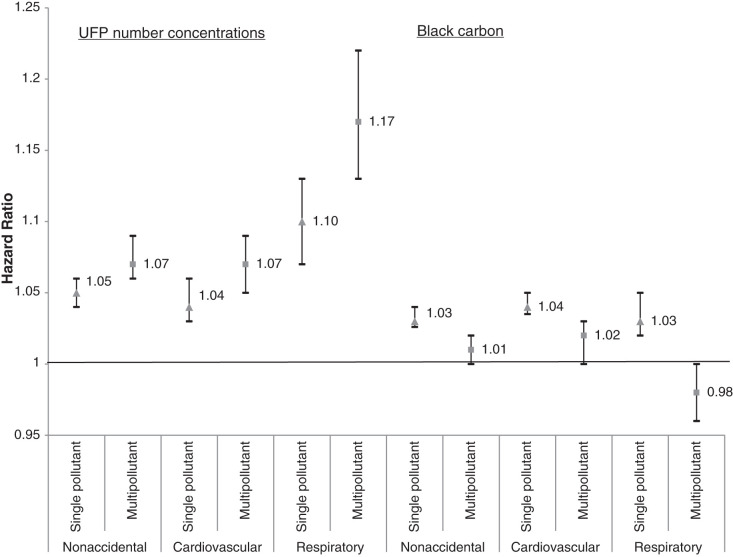
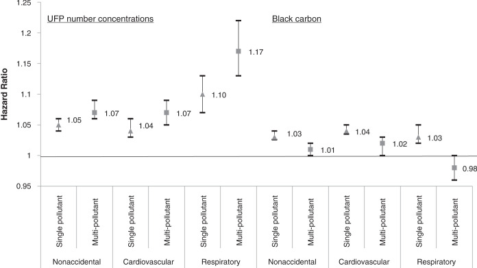
Using the combined exposure model with backcasting, the investigators documented that long-term exposures to UFP number concentrations and black carbon were positively associated with mortality in single-pollutant models. However, these results were sensitive to adjustment for co-pollutants and UFP size. Associations between UFP number concentrations and mortality increased after adjusting for UFP size, whereas associations between black carbon and mortality became generally weaker or null (Statement Figure).

Statement Figure. — Adjusted hazard ratios for UFP number concentrations (per 10,000 particles/cm³) and black carbon (per 500 ng/m³) and selected mortality outcomes using the combined exposure model with backcasting.

Generally, similar findings were reported for black carbon across various alternative exposure assessment approaches, including without backcasting and accounting for mobility patterns. For UFP number concentrations, the association’s magnitude — but not the direction — differed substantially across the various alternative exposure approaches.

INTERPRETATION AND CONCLUSIONS

In its independent review of the study, the HEI Review Panel thought the research was well-motivated and addressed a clear research gap because there are few long-term air pollution and health studies on UFPs. The extensive year-long mobile monitoring campaign and the rigorous development and innovative features of the new high-resolution models were considered to be strengths of the study. Another strength was the use of a large representative sample of Canadian adults to evaluate the sensitivity of the epidemiological analyses to different exposure assessment approaches.

Although the Panel broadly agreed with the investigators’ conclusions, some limitations should be considered when interpreting the results. Importantly, the adjustment for UFP size in health analyses of outdoor UFP number concentrations and black carbon was intriguing. However, it remains unclear how to interpret UFP size and this remains an area that warrants further research. More advanced multipollutant statistical approaches might be needed to capture the complex relationships across the different pollutants. The monitoring and exposure assessment approaches contained some uncertainties, such as the lack of fixed-site monitoring and the temporal mismatch between the period captured by the mobile measurements and the exposure window most relevant for epidemiological purposes. The findings in the current study of two Canadian cities might not be generalizable to other settings, partly due to distinct characteristics of these cities.

In summary, data from mobile monitoring are useful for developing high-resolution machine learning models and other exposure models but can have important limitations. Therefore, careful consideration is needed when using them in exposure assessment or epidemiological analyses.

Res Rep Health Eff Inst. 2024 Jul 1;2024:217.

Long-Term Exposure to Outdoor Ultrafine Particles and Black Carbon and Effects on Mortality in Montreal and Toronto, Canada

Scott Weichenthal ¹, Marshall Lloyd ¹, Arman Ganji ², Leora Simon ¹, Junshi Xu ², Alessya Venuta ¹, Alexandra Schmidt ¹, Joshua Apte ^3,⁴, Hong Chen ⁵, Eric Lavigne ⁵, Paul Villeneuve ⁶, Toyib Olaniyan ⁷, Michael Tjepkema ⁷, Richard T Burnett ⁵, Marianne Hatzopoulou ²

ABSTRACT

Introduction

Numerous studies support an important relationship between long-term exposure to outdoor fine particulate air pollution (PM_2.5^*) and both nonaccidental and cause-specific mortality. Less is known about the long-term health consequences of other traffic pollutants, including ultrafine particles (UFPs, <0.1 μm) and black carbon (BC), which are often present at elevated concentrations in urban areas but are not currently regulated. Knowledge is lacking largely because these pollutants generally are not monitored by governments and vary greatly over small spatial scales, hindering the evaluation of long-term exposures in population-based studies.

Methods

We aimed to estimate associations between long-term exposures to outdoor UFPs and BC and nonaccidental and cause-specific mortality in Canada’s two largest cities, Montreal and Toronto. We considered several approaches to exposure assessment: (1) land use regression (LUR) models based on large-scale year-long mobile monitoring campaigns combined with detailed land use and traffic information; (2) machine learning (i.e., convolutional neural networks [CNN]) models trained by combining mobile monitoring data with aerial images; and (3) the combined use of these two approaches. We also examined exposure models with and without backcasting based on historical trends in vehicle emissions (to capture potential trends in pollutant concentrations over time) and with and without accounting for neighborhood-level mobility patterns (based on travel demand surveys). These exposure models were linked to members of the Canadian Census Health and Environment Cohorts (CanCHEC) residing in Montreal or Toronto (including census years 1991, 1996, 2001, and 2006) with mortality follow-up from 2001 (or cohort entry for the 2006 cohort) to 2016. Cox proportional hazard models were used to estimate associations between long-term exposures to outdoor UFPs and BC, adjusting for sociodemographic factors and co-pollutants identified as potential confounding factors. Concentration-response relationships for outdoor UFPs and BC were also examined for nonaccidental and cause-specific mortality using smoothing splines.

Results

Our cohort study included approximately 1.5 million people with 174,200 nonaccidental deaths observed during the follow-up period. Combined LUR and machine learning model predictions performed slightly better than LUR models alone and were used as the main exposure models in all epidemiological analyses. Long-term exposures to outdoor UFP number concentrations were consistently positively associated with nonaccidental and cause-specific mortality. Importantly, hazard ratios (HRs) for outdoor UFP number concentrations were sensitive to adjustment for UFP size: UFP size was inversely related to number concentrations and independently associated with mortality, resulting in underestimation of mortality risk for outdoor UFP number concentrations when UFP size was excluded. HRs for outdoor UFP number concentrations were robust to backcasting and mobility weighting but varied slightly in analyses using LUR and machine learning models alone, with stronger associations typically observed for the machine learning models. Associations between outdoor BC concentrations and mortality were generally weak or null, but a positive association was observed for cardiovascular mortality.

Conclusions

Outdoor UFP number concentrations were consistently associated with increased risks of nonaccidental and cause-specific mortality in Montreal and Toronto. Our results suggest that UFP size should be considered in epidemiological analyses of outdoor UFP number concentrations, as excluding size can lead to an underestimation of health risks. Our results suggest that outdoor UFP number concentrations are positively associated with mortality independent of other outdoor air pollutants, including PM_2.5 mass concentrations and oxidant gases (i.e., nitrogen dioxide [NO₂] and ozone [O₃]). As outdoor UFPs are currently unregulated, interventions targeting these pollutants could significantly affect population health.

INTRODUCTION

Outdoor PM_2.5 is a leading contributor to the global burden of disease,¹ but less is known about the long-term health effects of other particulate air pollutants, including UFPs and BC. Outdoor UFPs contribute little to particle mass concentrations; consequently, exposures are typically measured as UFP number concentrations (i.e., number of particles/cm³). Extremely high numbers of UFPs can be present in a given volume of air (e.g., hundreds of thousands of particles/cm³), and these particles deposit efficiently in human lungs where they contribute to oxidative stress and inflammatory responses.^2–5 Furthermore, UFPs can translocate from the lung into the systemic circulation where they can trigger inflammatory responses throughout the body, including in the heart and brain.^3,5–8 Additional evidence suggests that UFPs can reach the brain directly via translocation through the olfactory nerve.^8–11

To date, a small number of studies have used LUR models^12–16 to evaluate the long-term health effects of outdoor UFPs, and existing evidence supports possible associations with incident myocardial infarction, heart failure, hypertension, and brain tumors with less consistent evidence observed for respiratory outcomes.^17–20 Although these studies generally suggest that long-term exposures to outdoor UFPs may have important health effects, the LUR models used in the previous North American studies are limited in a number of ways. First, these models were based on mobile monitoring data collected during morning (7–10 a.m.) and evening routes (3–6 p.m.) on weekdays.^12,13,21,22 As a result, these models likely overestimate true long-term exposures, as they do not capture evenings and weekends when outdoor UFP concentrations may be lower. Moreover, this limitation may obscure estimates of absolute concentration levels relevant to health outcomes, particularly if threshold-type concentration-response relationships are present. A second limitation of these models is that they were not backcast to estimate historical UFP concentrations; as a result, previous analyses assumed a constant spatial distribution over time, which likely contributed to exposure measurement error in the analyses. Other studies of the long-term health effects of UFPs also have important limitations. Specifically, Ostro and colleagues reported a positive association between outdoor UFP concentrations and ischemic heart disease mortality in the California Teachers Study Cohort, but the spatial resolution of exposure estimates in this study was 4 km.²³ Given the high spatial variability of UFPs within cities, a 4-km scale is too broad to capture fine-scale spatial variations in population-level exposures. Similarly, Pond and colleagues¹⁶ reported positive associations between outdoor UFPs and nonaccidental and cause-specific mortality on a national level in the United States, but exposures were aggregated to the census tract level, and HRs for UFPs were sensitive to the inclusion of PM_2.5. More recently, a cohort study in the Netherlands¹⁵ reported positive associations between long-term exposures to outdoor UFPs and nonaccidental and cause-specific mortality (e.g., respiratory, cardiovascular, and lung cancer), but correlations between UFP number concentrations and other air pollutants were sometimes high, and information on UFP size was not included. None of the existing epidemiological studies for outdoor UFP number concentrations include data for UFP size. This limitation is important because UFP size could be an important confounding variable in epidemiological studies of outdoor UFP number concentrations given that UFP size is inversely correlated with UFP number concentrations (i.e., particles tend to be smaller at higher number concentrations) and could be independently associated with mortality (i.e., at a given number concentration, smaller UFPs may be more harmful than larger UFPs, or vice versa). As such, failure to adjust for UFP size in epidemiological analyses could bias health risk estimates for outdoor UFP number concentrations. This issue also relates more broadly to issues of confounding when examining exposures with multiple versions of treatment,^24,25 which is discussed in more detail later in this report.

Compared to outdoor UFPs, more studies have examined the long-term health effects of outdoor BC concentrations. In particular, a meta-analysis of eight epidemiological studies reported a 6.1% (95% CI: 4.9, 7.3) increase in all-cause mortality per 1-μg/m³ increase in outdoor elemental carbon (EC)/BC concentrations.²⁶ A more recent study also reported a positive relationship between BC and cardiovascular mortality using a dispersion model to estimate exposures.²⁷ However, in their meta-analysis, Hoek and colleagues²⁶ noted that most existing studies of EC/BC estimated exposures at the city scale and did not account for small-scale spatial variations related to land use or built environment factors such as proximity to major roads. Capturing small-scale spatial variations in pollutant concentrations is a major challenge in studies of the long-term health effects of traffic-related air pollutants, and our project addressed this challenge in several important ways.

Specifically, we developed new exposure models to predict long-term exposures to outdoor UFPs (number concentrations and particle size) and BC across Canada’s two largest cities, Toronto and Montreal, using mobile monitoring campaigns conducted over an entire year, including all days of the week and most times of the day. Next, we developed new exposure models combining both traditional (i.e., LUR) and machine learning methods (i.e., CNN) using digital images²⁸ and applied these models (both separately and combined) in a new epidemiological study of outdoor UFPs and BC and nonaccidental and cause-specific mortality in the CanCHEC. As part of this process, we examined how different exposure modeling approaches affected observed associations between outdoor UFPs and BC and mortality as well as the sensitivity of health risk estimates to neighborhood-level mobility patterns and backcasting exposures over the duration of follow-up. Concentration-response curves for long-term exposures to outdoor UFPs and BC and mortality were also generated to evaluate the shapes of these relationships.

SPECIFIC AIMS

The overall objective of this study was to estimate associations between long-term exposures to outdoor UFPs and BC and mortality in Montreal and Toronto, Canada, including an evaluation of several different exposure modeling approaches. Our specific aims were as follows:

To develop new exposure models to predict within-city spatial variations in long-term average outdoor UFPs and BC in Montreal and Toronto, Canada, using data collected during large-scale mobile monitoring campaigns — New models included traditional LUR models, machine learning models trained using aerial images labeled with pollutant measurements, and combined models. Mobile NO₂ and O₃ and fixed-site UFP and BC monitoring were also conducted, but equipment failures and COVID-19 restrictions resulted in incomplete monitoring and precluded incorporation into the health analysis (lessons learned related to equipment failures are described in Appendix B; available on the HEI website).
To generate backcasted exposure estimates for outdoor UFPs and BC based on historical traffic emissions data
To compare and quantify differences between our final UFP model predictions and past models developed for UFPs in Montreal and Toronto that were based on mobile monitoring limited to weekdays and rush hour periods
To integrate mobility data into our exposure models through the development of mobility-weighted exposure surfaces that capture neighborhood-level trends in population mobility (and changes in mobility patterns over time) informed by travel survey data collected from random samples of Montreal and Toronto residents every 5 years
To link new UFP and BC exposure models (i.e., LUR models, machine learning models, and combined models with and without mobility weighting and with and without backcasting) to the CanCHEC cohort to estimate associations with nonaccidental and cause-specific mortality adjusting for relevant confounding factors and other outdoor air pollutants (i.e., PM_2.5, O_x)

CHANGES TO THE ORIGINAL STUDY AIMS

Our original plan was to compare our new models to past measurements for outdoor UFPs and BC and new fixed-site measurements collected concurrently with mobile monitoring, but we reconsidered this approach for several reasons. First, existing historical measurements for outdoor UFPs and BC do not adequately reflect true annual average outdoor concentrations (e.g., because monitoring was limited to weekdays, during daytime hours, with limited annual coverage), and thus differences between historical measurements and predicted values from our new models would be strongly influenced by systematic differences in the design of the previous sampling campaign and our new campaign. Therefore, instead of comparing our new models to past measurements, we compared our new UFP models to past UFP models in Montreal and Toronto.^12,13 The purpose of this analysis was to identify potential systematic differences in predictions across each study area to aid in interpreting any future discrepancies in the results of epidemiological analyses based on the new models. This comparison provides important information on spatial differences in predicted long-term average outdoor UFP number concentrations resulting from a more rigorous monitoring scheme including all days of the week and most times of day (our new model) and a past scheme with a more limited sampling protocol.^12,13 This comparison was only conducted for UFPs because past models do not exist for BC in Montreal and Toronto. Second, we did not compare our new model predictions to fixed-site UFP or BC measurements collected concurrently with mobile monitoring because we were unable to conduct winter fixed-site measurements owing to COVID-19 restrictions that prevented in-person work (i.e., working together in the laboratory or driving together in vehicles used to set up and take down fixed-site monitors). The fixed-site data we collected were limited to 2 weeks during the summer months in each city and does not reflect a long-term average. Moreover, many of the UFP instruments failed during fixed-site monitoring owing to issues related to high relative humidity.

NO₂ and O₃ mobile monitoring was limited by technical issues with the monitoring equipment, and we were unable to develop new models for outdoor NO₂ and O₃ in Montreal (additional information in the lessons learned section of Appendix B). However, we completed several additional tasks that were not originally proposed. First, two levels of NO₂ and O₃ sensor calibration were implemented, both in a chamber and in the field, against reference instrumentation.²⁹ Using chamber test data, a set of mathematical tools were developed to correct for sensor noise (wavelet denoising), misalignment (linear and nonlinear), and hysteresis. A predesigned sampling strategy, based on spatial and statistical methods, was also developed. With respect to UFPs, we developed a machine-learning model to predict short-term UFP exposures using street-level images.³⁰ We did so by extracting features from images, which were averaged over 10 seconds, and combining them with regional air quality and meteorological data gathered from a fixed station in Toronto.³⁰

Finally, we added UFP size to our exposure modeling and epidemiological analyses to address concerns related to confounding bias caused by UFP size. Specifically, because UFPs tend to be smaller at higher number concentrations and particle size is likely related to toxicity, confounding by UFP size seems possible and could result in underestimation or overestimation of the health effects of outdoor UFP number concentrations depending on the direction of the association with the outcome.³¹ The issue of UFP size relates to the broader topic of exposures with multiple versions of treatment and confounding of version of treatment–outcome associations, which is addressed in previous publications.^24,25 Specifically, because outdoor UFP number concentrations have multiple versions of treatment (i.e., the same UFP number concentration can be constructed with many different size distributions, which may vary in toxicity), we must account for possible confounders of the version of treatment–outcome associations to avoid confounding bias in health risk estimates for outdoor UFP number concentrations. In this case, UFP size is a likely confounder of the version of treatment–outcome relationships for outdoor UFP number concentrations and mortality because UFP size is a cause of the version of treatment for outdoor UFP number concentrations (i.e., the kinds of UFPs present) and could also be independently associated with the outcome (i.e., smaller UFPs may be more harmful than larger UFPs, or vice versa). If we do not adjust for this source of confounding bias, health risk estimates for outdoor UFP number concentrations will reflect some unknown combination of both the total number concentration and the version of treatment (i.e., the number of particles present and the kinds of particles present). With this in mind, all of the exposure models mentioned previously were developed for UFP size, and UFP size was included in all epidemiological analyses. This is the first study to simultaneously consider both UFP number and UFP size in epidemiological analyses examining mortality.

STUDY DESIGN AND METHODS

STUDY LOCATIONS

Our study was conducted in the cities of Montreal and Toronto, Canada. The Montreal study area included all municipalities on the island of Montreal (population 2.0 million in 2021), and the Toronto study area included the post-amalgamation political border of the city of Toronto (population 2.8 million in 2021). Both cities border major bodies of water, are surrounded by large suburban communities, and have similar climates (Appendix A, Table A.1; available on the HEI website).

EXPOSURE MODEL DEVELOPMENT AND EVALUATION

Mobile Monitoring

We conducted year-long (September 2020 to August 2021) mobile monitoring campaigns for outdoor UFP number concentrations, UFP size, and BC. Monitoring routes (Appendix A, Figure A.1) were designed to capture a wide variety of land use and road types. This was done by dividing the study areas into 100 m × 100 m grids, extracting land use and traffic parameters for each grid square, and conducting a principal component analysis to identify clusters that explain the greatest amount of variance in the data (additional methodological details are described in Appendix B). Routes were then selected along multiple road types within each of the clusters. To obtain measurements representative of annual averages, these prespecified routes were monitored repeatedly at various times of day between 7 a.m. and 11 p.m. on all days of the week, including weekends, and in all four seasons. We randomly selected the time of day, day of week, and order in which routes were monitored each week. Each monitoring route took approximately 1 hour, and 3 to 15 routes were completed each week.

Fixed-Site Monitoring

As noted previously, fixed-site monitoring was not possible during the winter months of 2021 because of the COVID-19 pandemic (i.e., social distancing requirements prevented laboratory and field work). Consequently, fixed-site monitoring data were limited to summer 2021. As a result, these data were not used for model development or evaluation. Details on the procedures used for fixed-site monitoring are available in Appendix B. Descriptive data for monitoring results from fixed sites are presented in Appendix A, Table A.2 but are not otherwise used or discussed in this report.

Air Pollution Measurements

UFP and BC monitors were time-synched with global positioning system monitors and sampled data at 1-second resolution. The BC monitor was a microAeth MA350 (https://aethlabs.com/microaeth/ma350/tech-specs). The UFP monitors were the Naneos Partector 2 (https://www.naneos.ch/partector2.html) and Testo DiSCmini (https://www.testo.com/en-US/testo-discmini/p/133). Both monitors concurrently measure UFP number concentrations (particles/cm³) and mean UFP size (nm) at a set sampling interval (i.e., 1 sec) using the same operating principles and were factory-calibrated for the monitoring campaign. Mean UFP size (referred to as UFP size throughout this text) was the mean diameter of UFPs sampled during the sampling interval and was measured by the monitors using a factory-calibrated ratio of currents from charged ultrafine particles.³² This approach is different from that of other UFP monitors in that it does not estimate the entire size distribution of sampled UFPs. Instead, it gives a single value for mean UFP size during the sampling interval using an assumed particle size distribution. Fierz and colleagues conducted roadside measurements using this approach and a scanning mobility particle sizer and observed that mean UFP size measurements from both instruments were highly correlated (R² = 0.99).³² We treated data from both the Testo DiSCmini and Naneos Partector 2 as equivalent because both monitors measure UFPs using the same operating principles and were factory-calibrated for the monitoring campaign.

For each mobile monitoring run, a BC monitor was mounted on the roof of the vehicle, and a UFP monitor was mounted inside the vehicle (Nissan Micra for Toronto and Nissan Rogue for Montreal) with a sampling tube inlet extended out the rear passenger-side window and pointed downward to prevent water from entering the instrument. The tube inlets were roughly 2 m above and in front of the vehicle tailpipes, but the vehicle emissions may have increased air pollution concentrations at the tube inlet. However, it is important to note that we observed UFP concentrations below 1,000 particles/cm³ and BC concentrations below 50 ng/m³, suggesting that this contribution was not substantial. After each monitoring run, instruments were inspected and the data were offloaded to local and cloud data storage. Files were inspected, and data points associated with instrument error codes or implausible temporal or spatial patterns (e.g., constant concentrations) were removed from the analysis. Values above and below the manufacturer’s reported limits of detection (listed in Appendix Table A.3) were replaced with the upper and half of the lower limit of detection, respectively. Instrument drift was assessed by conducting monthly zero checks. The monitoring quality assurance plan is described in Appendix B.

Data Preprocessing

Air pollution and geospatial position data were joined by matching time stamps. Hourly average ambient weather conditions recorded at Automated Surface Observing Systems within each study area (Appendix Table A.4) were downloaded using the riem package (https://docs.ropensci.org/riem) in version 4.1.2 of the R statistical computing environment (R Core Team, Vienna, Austria) and matched to the monitoring data by time. Road networks in each city were divided into 100-m road segments. The median of all 1-second air pollution measurements along a given road segment (i.e., the grand median) and the median ambient weather conditions during monitoring were assigned to the centroid of the road segment. The median air pollution levels were our estimates of annual median ambient pollutant levels and are referred to as the observed values for the remainder of this text. The unit of analysis for this study was annual median ambient pollutant levels at the 100-m road segments (i.e., the temporal median of all monitoring data along each 100-m road segment). Road segments monitored on fewer than six separate days throughout the campaign were excluded from the analysis. This value was selected as a reasonable trade-off between improving temporal stability and maximizing spatial coverage. In total, mobile monitoring data were aggregated to 7,051 and 5,819 road segments in Montreal and Toronto, respectively.

Six-digit geohash codes were assigned to each road segment based on their location, and road segments were randomly split by geohash code into training (70%), validation (15%), and test (15%) sets. The geohash geocoding system spatially splits the globe into cells, each with its own alphanumeric code. A cell with a six-digit geohash code is approximately 1.22 km by 0.61 km. Stratifying the random split by geohash code (i.e., geospatial position) increases the independence of the test set and reduces the overlap of images from the training, validation, and test sets (Appendix Figure A.2), which was crucial for training machine learning models. The distributions of observed UFP number concentrations and BC concentrations were right-skewed and were log-transformed for model development. The distribution of observed UFP size was not skewed and was not log-transformed.

Image Data for Training CNN

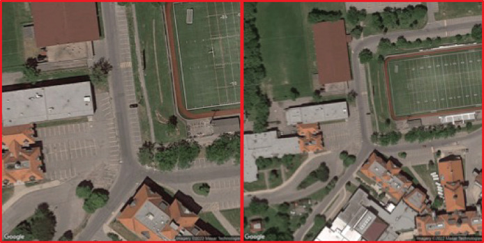
For each road segment centroid, two aerial (i.e., satellite-view) images were downloaded from Google maps at different zoom levels (18 and 19) using the ggmap package (https://rdrr.io/cran/ggmap) in R. Zoom 18 and 19 images covered areas of approximately 280 m × 280 m and 140 m × 140 m, respectively. Figure 1 shows an example of images at different zoom levels for a particular road segment. All CNN models included two images as inputs to capture both local (zoom 19) and contextual (zoom 18) information. Images were downloaded with a resolution of 604 × 640 × 3 (i.e., image height by width by color channels) and then resized (256 × 256 × 3) and linked to the monitoring data for CNN model training. Image resizing was needed to produce an input image size suitable for use with the Xception model architecture described below.

Figure 1. — Example of zoom 19 images (left) and zoom 18 images (right) for a given road segment.

For readers unfamiliar with CNNs, a single color image can be thought of as three 256 × 256 arrays, one for each color channel (red, blue, and green). Each value in each array corresponds to the intensity of a particular color for a given pixel of the image. The CNN algorithm performs a large number of mathematical transformations on the numeric values in these arrays (i.e., the pixel data of the images), and, through an iterative process, the CNN learns features in the digital images that are associated with the desired target (i.e., outcome). In this application, the images were color satellite-view images centered on road segments, and the target was air pollution levels measured at the road segment. Thus, the raw data of digital satellite-view images were the numeric values of the 256 × 256 × 3 arrays, and the mathematical transformations may identify different features (i.e., patterns of numbers in the arrays), such as roads, if those features are associated with air pollution in the training data. The specific mathematical transformations performed by a given CNN algorithm will depend on the CNN’s model architecture, and the importance assigned to the various transformations is the CNN’s model weights (i.e., the model parameters). For each iteration during model training, the weights are updated using an optimizer algorithm intended to minimize the difference between the measured target value and the CNN predicted target value. Various model architectures, initial model weights, and optimizers have been developed by deep learning scientists and are available for use in a variety of applications.

Land Use and Traffic Data

Land use and traffic data were extracted using ArcMap 10.8.1 (Environmental Systems Research Institute Inc., Redlands, CA, USA). Data sources included DMTI Spatial (Richmond Hill, CA), EMME (INRO, Montreal, Canada), City of Montreal, City of Toronto, Canadian National Pollution Release Inventory, Statistics Canada, Toronto Transit Commission, and Société de Transport de Montréal. Examples of predictor variables included average traffic nitrogen oxides (NO_x) emissions within 300 m, length of railroad within 100 m, residential area within 200 m, and distance to the nearest highway. Appendix Table A.5 describes all 32 spatial predictor variables examined in this study (buffers examined were 100 m, 200 m, and 300 m). LUR models were developed using contemporary land use and traffic values.

Historic Traffic Data

Traffic data were predicted using the traffic emission prediction scheme from 2006 to 2020.^33,34 This approach uses statistical methods and machine learning techniques to generate yearly traffic counts and traffic-related NO_x emissions from long-term and short-term traffic counts and aerial images (additional details in Appendix B). Historical values of traffic NO_x emissions for Toronto (2006–2016) and Montreal (2008, 2013) were used to project model predictions back in time (i.e., backcast) given that traffic-related pollutants such as UFPs and BC are strongly related to traffic NO_x emissions (our past studies). For backcast predictions, the other selected variables in the LUR models were land use variables, which typically have been stable for Montreal and Toronto over the past two decades. For example, railroads, airports, major highways, residential areas, and industrial areas have largely been in the same locations since 2000.

Data Used for Mobility-Weighted Exposure Models

Travel-demand survey data from the Authority Régionale de Transport Métropolitain³⁵ and the Transportation Tomorrow Survey³⁶ were used to weight exposure surfaces to produce mobility-weighted surfaces. These population-weighted surveys provided neighborhood-level (i.e., dissemination area) average proportions of time spent away from home and in which neighborhoods that time was spent. The Transportation Tomorrow Survey (Toronto) data were available for 2001, 2006, 2011, and 2016. The Authority Régionale de Transport Métropolitain (Montreal) data were available for 2003, 2008, and 2013. Exposure estimates in mobility-weighted models reflect a weighted average based on the proportion of time spent at home and the estimated proportion of time spent away from home in a given location based on travel-demand survey data.

LUR Model Development

Generalized additive models³⁷ (e.g., https://rdrr.io/cran/mgcv) were developed for each city to predict spatial variations in annual average outdoor UFP number concentrations, UFP size, and BC concentrations. Variable selection and model training were conducted using the training datasets following the same method for all three measures of outdoor air pollution. Regional median ambient temperature, relative humidity, and wind speed during monitoring along each road segment were included in all models to account for weather-related temporal variations in air pollution during the monitoring campaign. Our monitoring campaign was designed to be temporally balanced, but due to the relatively low number of visits at certain sites (i.e., as few as six visits), some temporal imbalances occurred between sites. We used temporal adjustment to account for chance weather-related temporal variations in the monitoring data while developing purely spatial models. First, air pollution levels were regressed onto each land use parameter (listed in Appendix Table A.5), including the weather variables in the model. Parameters associated with the air pollutant (95% CI excluding the null) without being driven by outliers (predictor variable values greater than 2 SD from the mean) became candidate variables. All outliers were retained for all model development. To reduce possible collinearity, pairs of correlated candidate variables were identified (Spearman’s correlation >0.7), and those with a lower mean square error (MSE) in the regression models were selected for inclusion in the final LUR models. All LUR models were trained as Generalized additive models estimated using restricted maximum likelihood, and thin plate splines were used to allow for nonlinear relationships (limited to three basis functions to avoid overfitting). Additional spatial dependencies not captured by land use and traffic parameters were modeled by including road segment latitude and longitude in a tensor product smooth, as described by Wood³⁸ (models without latitude and longitude were also developed as a sensitivity analysis).

CNN Model Development

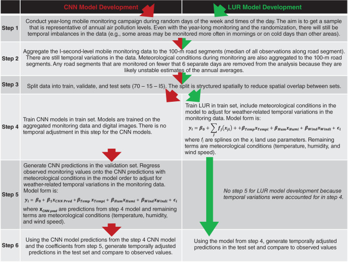
CNN models for UFPs (number concentration and size) and BC were developed using satellite-view images at two different zoom levels. The keras package³⁹ (https://keras.io) in Python was used to train models on the training set data (70%; 9,300 images for Montreal and 7,330 images for Toronto), and hyperparameter tuning was based on MSE in the validation set (15%). The Xception model architecture⁴⁰ with ImageNet initial weights⁴¹ and the Nadam learning rate optimizer was used.⁴² The initial learning rate was 0.0001 and was reduced if MSE in the validation set plateaued for five epochs. The batch size was 128 (32 images per GPU), and models were trained for up to 100 epochs (training was stopped early if MSE in the validation set plateaued for 10 epochs). Model weights that resulted in the lowest MSE in the validation set were selected. Because the CNN predictions did not account for weather-related temporal variations in the monitoring data, we used the same approach as a previous study⁴³ whereby observed air pollution levels are regressed onto the CNN predictions in the validation set with median ambient weather conditions during monitoring included in the model to account for weather-related temporal variations in air pollution (steps illustrated in Figure 2). The coefficients from this regression were used to adjust CNN model predictions for temporal variations in the monitoring data. As sensitivity analyses, the LUR models were trained using the same approach for temporal adjustment (i.e., training the model in the training set without weather parameters and then adjusting for weather-related temporal variations in the validation set), and both LUR and CNN models were trained without any temporal adjustment. All outliers were retained for all model development.

Figure 2. — **Steps used to develop LUR and CNN models.** The combined model had an additional step of regressing the step 7 LUR and CNN predictions onto observed values in the validation set. CNN = convolutional neural network; LUR = land use regression.

Combined Model Development

Final combined models for UFP number concentrations, UFP size, and BC in each city were developed by combining LUR model predictions with the temporally adjusted CNN model predictions. This was done using a linear regression model in the validation set:

where x_LUR and x_CNN are predictions from the LUR and CNN models respectively (nonlinear models did not improve model performance). These combined models captured information from both the LUR and CNN models.

Model Evaluation

We developed city-specific LUR, CNN, and combined models for each pollutant in each city. As a sensitivity analysis, multicity models were developed by pooling data from both cities. Predictions (i.e., estimates) from each model were generated in the test set and compared to observed values. Root mean square error (RMSE) and R² values were used to describe model performance. Model residuals for all data were plotted and inspected for spatial clustering.

Prediction Surfaces

Study areas were divided into 100 m × 100 m cells for the prediction surfaces. For each cell, land use and traffic parameters were extracted and used to generate LUR model predictions, and satellite-view images at both zoom levels were downloaded to generate CNN model predictions. Spatially invariant (i.e., constant) annual median temperature, humidity, and wind speed at local airports (i.e., the same data source used for weather conditions during monitoring) were used for each city when generating predictions. Using invariant values assumes a spatially constant temporal structure across the study areas and also assumes that predictions of pollutant levels under average regional meteorological conditions represent annual median outdoor pollutant levels. Surfaces from the combined models provide estimates of within-city spatial variation of annual ambient pollution (i.e., UFP number concentration, UFP size, and BC mass concentration).

Examining CNN Model Behavior

CNN models lack the easily interpretable coefficients of regression models; thus, we explored model behavior using an approach described by Sorek-Hamer and colleagues,⁴⁴ which involved modifying digital images and qualitatively comparing predicted values to expected values. For example, pasting the image of a highway into the image of a residential area was expected to increase the predicted UFP concentration for the unmodified residential area. The resulting prediction was compared to expectations to determine if the model behaved in a manner consistent with expectations. In addition, we generated CNN model predictions using images from different time periods (Google periodically updates satellite-view images) to explore the sensitivity of CNN models to the time of year in which an image was captured.

Code Availability for CNN Models

Python code used for training CNNs is available online: https://github.com/Sweichenthal/HEI-19-1. Additional information on training CNNs using the keras package in Python is available elsewhere.⁴⁰

Comparison of New UFP Surfaces to Old UFP Models

To compare predicted annual average outdoor UFP number concentrations between our new models and previous surfaces,^12,13 we first used the spatial join function in ArcGIS to align previous model results (based on data collected in 2010–2012) with the polygon shapefiles from our new models. We standardized UFP levels predicted by each surface (i.e., subtracting each model’s mean value and dividing by its standard deviation) to facilitate comparisons. We also generated maps of differences in predicted outdoor UFP number concentrations on the original scale. Given the systematic differences between the monitoring campaigns used to develop the models (i.e., weekday rush hours only vs. all days and most times of day), we did not compare our backcasted estimates to historical models.

EPIDEMIOLOGICAL ANALYSIS

Study Population and Mortality Outcomes

Our study population included multiple cycles (1991, 1996, 2001, and 2006) of the CanCHEC. This dataset was formed by linking census long-form questionnaires (which collect data on approximately 20% of Canadian households every 5 years) to postal code histories and mortality records through the Statistics Canada Social Linkage Data Environment.^45–47 Follow-up included the 15-year period between 2001 and 2016, and the in-scope study population included noninstitutionalized respondents (at the time of census collection) under the age of 90 who lived in Toronto or Montreal for at least 1 year between 1998 and the end of 2016. Participants were censored at the time of death, end of follow-up, or movement out of Montreal or Toronto. Residential postal code histories (from mailing addresses reported on annual income tax filings) were used to account for residential mobility both within and between cities. We examined associations between outdoor UFPs and BC and several causes of death, including nonaccidental (International Classification of Diseases, Tenth Revision (ICD-10): A–R), cardiometabolic (i.e., circulatory plus diabetes; ICD-10: I10–I69, E10–E14), cardiovascular (ICD-10: I10–I69), ischemic heart disease (ICD-10: I20–I25), cerebrovascular (ICD-10: I60–I69), nonmalignant respiratory (ICD-10: J00–J99), and lung cancer (ICD-10: C33–C34). The creation of the CanCHEC dataset was authorized by Statistics Canada senior management (reference number: 019-2019) as per the Directive on Microdata linkage.

Exposure Assignment

All of the exposure models described for UFP number concentrations, UFP size, and BC mass concentrations were linked to cohort members using six-digit residential postal codes (about the size of a city block face). The 3-year moving average exposures were used with a 1-year lag; time-varying exposures were used to account for residential mobility within and/or between cities. The 1-year lag ensures that estimates of long-term exposures precede the outcome given that postal codes in CanCHEC are updated at year-end. The same approach was used to assign exposures to outdoor PM_2.5 mass concentrations and O_x (combination of NO₂ and O₃) using exposure models previously described.⁴⁸ Briefly, the PM_2.5 estimates were from satellite-based aerosol optical depth measurements that were subsequently adjusted using ground-based monitoring and land use data. NO₂ estimates were from a national LUR model, and the O₃ estimates were from a chemical transport model. NO₂ reacts with sunlight and oxygen to form O₃, and as such, ambient concentrations of NO₂ and O₃ are typically inversely correlated.⁴⁹ Previous research suggests that combining NO₂ and O₃ into a single measure of exposure to oxidant gases (O_x) is more relevant to mortality than treating them as separate exposures.^48,50,51 Following the approach of previous research,^48,50,51 exposure to oxidant gases (i.e., the combined oxidant capacity of NO₂ and O₃) was calculated using weights based on their approximate redox potential⁵²:

Exposures for outdoor UFP number concentrations, UFP size, and BC were backcasted using historical data for traffic emissions (i.e., NO_x) available for Toronto (2006–2016) and Montreal (2008, 2013). Our main analysis was based on combined CNN-LUR models (i.e., the best-performing models) using backcasted exposures assigned to residential locations. As sensitivity analyses, we also examined models with and without backcasting as well as models considering neighborhood-level mobility patterns. Specifically, mobility-weighted models were constructed using travel-demand survey data collected at the dissemination area level (stable geographic units with a population of approximately 400–700) by the Authority Régionale de Transport Métropolitain in Montreal and the Transportation Tomorrow Survey in Toronto.^35,36 These population-weighted surveys provided neighborhood-level average proportions of time spent away from home and in which neighborhoods that time was spent. Toronto data were available for 2001, 2006, 2011, and 2016. Montreal data were available for 2003, 2008, and 2013. Final mobility-weighted exposure surfaces reflected a weighted average based on the neighborhood-level proportion of time spent at home and the neighborhood-level proportion of time spent away from home in a given location based on travel-demand survey data.

Statistical Analysis

Cox proportional hazard models were used to estimate HRs for nonaccidental and cause-specific mortality. Follow-up time (with calendar time as the time-axis) was accrued beginning on census day 2001 (May 15, 2001) for 1991,1996, and 2001 CanCHEC members and cohort entry date for members of the 2006 CanCHEC (May 16, 2006). Cohort members were censored if they moved out of the study area (i.e., Montreal or Toronto), were lost to follow-up, reached the end of follow-up (December 31, 2016), or died from a cause other than an outcome of interest. Separate models were examined for each mortality outcome. All analyses were conducted for both cities combined, and city-specific analyses were not conducted.

The directed acyclic graphs shown in Appendix Figure A.3 describe the assumed relationship between the main outdoor air pollution concentrations of interest and mortality along with covariates identified and included as potential confounding factors or strata variables. Specifically, all models included terms for outdoor UFP number concentrations and BC mass concentrations and were stratified by age (5-year groups), immigrant status, sex, and census cycle and were additionally adjusted for education, occupational level, income, marital status, visible minority status, and other air pollutants (i.e., PM_2.5 and O_x.⁴⁸ Finally, all models were also adjusted for mean UFP size for reasons outlined previously. Penalized spline terms were used for UFP size to capture potential nonlinear associations between UFP size and mortality. Multiple pollutants were included in the Cox models to estimate independent associations between the pollutant of interest and mortality while controlling for exposure to co-pollutants. Interactions between pollutants (i.e., PM_2.5, O_x, UFP, and BC) were not explored. With UFP number concentration in a model, UFP size was considered an independent mortality risk (i.e., while controlling for UFP number concentration, variations in UFP size could be associated with mortality); thus, UFP size was included as a co-pollutant for the main analysis, which sought to estimate the independent risks of long-term exposure to UFPs and BC. As sensitivity analyses, linear and nonlinear (penalized splines with generalized cross-validation) terms were examined for UFP size to evaluate the impacts on mortality HRs for our main exposures of interest (reference exposures for nonlinear terms were the lowest exposures in the cohort). In addition, models excluding UFP size were also evaluated to examine the magnitude of possible confounding bias caused by not adjusting for this variable. To compare to previous studies, single-pollutant models were also examined for UFP number concentrations and BC. We did not examine single-pollutant models for UFP size, as we do not think it is appropriate to consider this pollutant on its own without UFP number concentrations also in the model.

Nonlinear concentration-response relationships for outdoor UFP number concentrations, UFP size, and BC were examined using penalized splines with generalized cross-validation to select the optimal smoothness parameters. The y-axis of the concentration-response curves was the HR, with the lowest cohort exposure as the reference exposure level. Multipollutant models were used for concentration-response curves, which included UFP number concentrations, UFP size, and BC as nonlinear terms. PM_2.5 and O_x were included in those multipollutant models as linear terms. STATA version 17.0 was used for all analyses except for estimating concentration-response curves, which was done using R version 4.0.5.

RESULTS

EXPOSURE MODEL DEVELOPMENT AND EVALUATION

We conducted more than 700 hours of mobile monitoring in Montreal and Toronto and retained more than 500 hours for model development. Less than 0.5% of BC and UFP measurements were imputed for being above or below instrument limit of detection. Monitoring data were retained for 12,870 road segments (7,051 in Montreal and 5,819 in Toronto) that were visited on at least six different days during the campaign (Appendix Tables A.6–A.7 and Figures A.4–A.5). Road segments (100 m) were visited on a median of 10 different days (SD = 8) and monitored for a median duration of 63 seconds in total (SD = 640). As shown in Table 1. Toronto had slightly higher median observed concentrations of UFP and BC and larger median observed UFP size. UFP number concentration, UFP size, and BC mass concentration were monitored concurrently, sampled at the same 1-second intervals, and aggregated to the same 100-m road segments for model development. Models for all three measures were developed using the same methods.

Table 1.

Descriptive Statistics for Mobile Monitoring Data for Road Segments with at Least 6 Days of Monitoring

Pollutant	City	Median (IQR)	1st–99th Percentile
UFP number (particles/cm³)	Toronto Montreal	16,172 (14,991) 14,702 (13,549)	5,008–110,139 3,377–81,623
UFP size (nm)	Toronto Montreal	33.7 (7.7) 29.7 (10.1)	19–50 15–53
BC (ng/m³)	Toronto Montreal	1,225 (1,151) 1,060 (1,006)	232–4,384 115–3,916

Open in a new tab

BC = black carbon; IQR = interquartile range; UFP = ultrafine particles.

Model Evaluation

Variables selected for each LUR model are listed in Table 2, and correlations between predictor variables are in Appendix Figures A.6–A.11. All city-specific model R² values and combined models coefficients are shown in Table 3 (RMSE values are shown in Appendix Table A.8). All models had generally similar performance, with combined models having the highest R² values. LUR and CNN model predictions were highly correlated (Appendix Table A.9), but the LUR models had slightly higher R² values. The LUR predictions also had slightly larger coefficients in the combined models (Table 3) and thus made greater contributions to the combined models than did the CNN predictions. All city-specific models had higher R² than the multicity models trained on pooled data (Appendix Table A.10). Conducting the LUR temporal adjustment in the validation set instead of the training set and omitting the temporal adjustment of LUR and CNN models had little impact on model R² values (Appendix Tables A.11 and A.12). Maps of median meteorological conditions during monitoring show some spatial variation (Appendix Figure A.12), and response curves for meteorological terms in the models (Appendix Figures A.13 and A.14) show relatively modest associations with pollutant concentrations across the monitoring sites.

Table 2.

Parameters Included in LUR Models

Parameter	Montreal			Toronto
Parameter	UFP number	UFP size	BC	UFP number	UFP size	BC
Average traffic NO_x emissions within 100 m			x	x	x	x
Total traffic NO_x emissions within 100 m	x	x
Building area within 100 m	x	x		x	x	x
Building area within 300 m			x
Length of bus routes within 100 m		x	x	x	x	x
Length of bus routes within 300 m	x
Number of bus stops within 100 m		x			x	x
Number of bus stops within 300 m			x
Commercial area within 100 m	x	x	x
Commercial area within 300 m						x
Distance to nearest highway			x
Distance to nearest NO_x NPRI chimney					x
Distance to nearest PM NPRI chimney	x	x	x	x	x	x
Distance to nearest port		x		x	x
Distance to nearest railroad	x			x		x
Distance to nearest shore	x	x	x
Governmental area within 100 m				x	x	x
Governmental area within 200 m			x
Governmental area within 300 m	x	x
Length of highways within 300 m	x	x
Industrial area within 300 m		x		x	x
Length of major roads within 100 m			x		x
Length of major roads within 300 m	x	x
Number of traffic intersections within 100 m	x	x	x		x
Number of traffic intersections within 200 m						x
Number of NO_x NPRI chimneys within 200 m	x	x			x
Number of PM NPRI chimneys within 200 m	x	x
Open area within 100 m	x	x	x
Open area within 300 m				x	x	x
Park area within 100 m				x	x
Population within 100 m	x		x
Population within 300 m		x		x	x	x
Length of railroad within 100 m				x
Length of railroad within 300 m		x			x
Residential area within 100 m	x	x	x	x	x	x
Number of restaurants within 200 m						x
Number of restaurants within 300 m	x	x	x	x
Length of roads within 200 m	x	x			x
Water area within 300 m	x	x	x
Latitude	x	x	x	x	x	x
Longitude	x	x	x	x	x	x
Temperature	x	x	x	x	x	x
Wind speed	x	x	x	x	x	x
Humidity	x	x	x	x	x	x

Open in a new tab

BC = black carbon; LUR = land use regression; NO_x = nitrogen oxides; NPRI = National Pollutant Release Inventory; PM = particulate matter; UFP = ultrafine particles.

Table 3.

Model Performance in Test Set and Combined Model Coefficients

City	Pollutant	R² in Test Set			Combined Model Coefficients
City	Pollutant	LUR	CNN	Combined	Intercept	LUR	CNN
Montreal	UFP number (particles/cm³) UFP size (nm) BC (ng/m³)	0.59 0.48 0.58	0.49 0.41 0.50	0.60 0.49 0.60	−0.25 1.49 −0.13	0.57 0.52 0.52	0.46 0.44 0.50
Toronto	UFP number (particles/cm³) UFP size (nm) BC (ng/m³)	0.71 0.56 0.60	0.66 0.43 0.53	0.73 0.55 0.61	−1.34 −2.34 −0.69	0.65 0.56 0.72	0.49 0.51 0.38

Open in a new tab

BC = black carbon; CNN = convolutional neural network; LUR = land use regression; UFP = ultrafine particles.

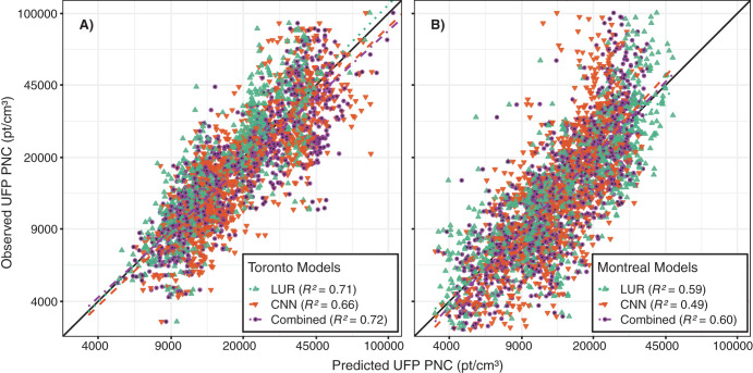
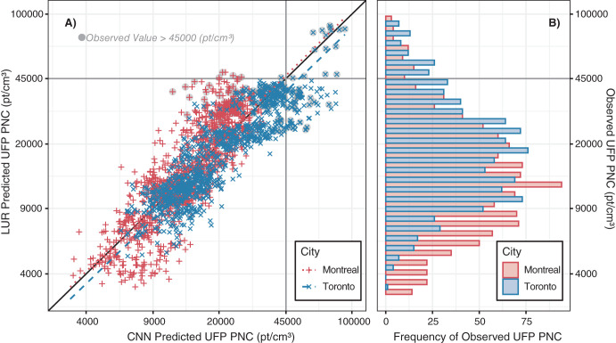
Table 4 shows median differences between observed values (i.e., aggregated monitoring data) and model predictions in the test set, and compared to the range of observed values of each pollutant, the mean differences were relatively small. The median differences for all the Montreal UFP concentration models were similar, but the Toronto LUR on average slightly underpredicted compared to observed values, whereas the Toronto CNN and combined models slightly overpredicted. For BC concentrations, all models slightly underpredicted on average. This contrast in LUR and CNN UFP concentration model behavior between cities was explored further in scatter plots of observed and predicted UFP number concentrations (Figure 3) and plots of LUR and CNN predictions (Figure 4, Appendix Figures A.15 and A.16, Appendix Tables A.13 and Table A.14). The Toronto CNN and combined UFP concentration models generated more predictions above 45,000 particles/cm³ than did the Toronto LUR model. Conversely, the Montreal LUR model generated a greater number of elevated UFP concentration predictions than did the CNN or combined model. This diverging pattern in UFP concentration predictions was much less pronounced when using multicity CNN and LUR models that were trained on both Montreal and Toronto data (Appendix Figures A.17–A.20). This suggests that the CNN UFP concentration model trained on Toronto data alone may have learned features specific to Toronto that were associated with elevated UFP concentrations (Appendix Figure A.21). BC mass concentration and UFP size predictions did not exhibit the diverging patterns observed for UFP concentrations in Figure 4 (Appendix Figures A.22–A.24). The Toronto LUR UFP concentration predictions exhibited unexpected clustering, but the Toronto CNN model predictions did not (Appendix Figure A.25). This was in part due to some of the test set data being clustered along major highways (Appendix Figures A.26 and A.27) that had distinctly elevated values of vehicle traffic (Appendix Figure A.28), which was an important variable the LUR model (Appendix Figure A.29). The same clustered test set did not lead to clustered CNN model predictions because CNNs are not trained on distinct categories of parameters but instead learn complex features in digital images. Slopes and intercepts of the scatter plots are listed in Appendix Table A.15. Model errors were mapped and did not appear to be spatially clustered (Appendix Figures A.30–A.32).

Figure 3. — **Comparing observed to predicted UFP number concentrations in Toronto (A) and Montreal (B) with legends showing model performance in the test set.** PNC = particle number concentration; UFP = ultrafine particles.

Figure 4. — **Comparing predictions for outdoor UFP number concentrations from LUR and CNN models in the test set in Montreal and Toronto.** The Pearson correlation between LUR and CNN model predictions was 0.80 for Montreal and 0.86 for Toronto (panel A). A histogram of observed values is shown in panel B for each city. CNN = convolutional neural network; LUR = land use regression; PNC = particle number concentration; UFP = ultrafine particles.

Table 4.

Median Difference Between Observed and Predicted Values in the Test Set and the 5th to 95th Percentile Range of Observed Values Used for Model Development (Aggregated Monitoring Data)

Pollutant	Model	Median Difference (5th, 95th percentile)		Observed 5th–95th Percentile Range
Pollutant	Model	Montreal	Toronto	Montreal	Toronto
UFP number (particles/cm³)	LUR	−338 (−11,332, 17,177)	533 (−12,285, 22,961)	41,195	46,815
	CNN	−232 (−8,948, 24,100)	−1,530 (−18,211, 16,988)
	Combined	−125 (−8,924, 21,220)	−770 (−20,864, 16,063)
UFP size (nm)	LUR	−0.35 (−9.18, 10.14)	−0.06 (−6.37, 6.80)	27	21
	CNN	−0.79 (−10.17, 11.83)	0.72 (−6.64, 8.75)
	Combined	−0.8 (−9.64, 10.20)	0.54 (−5.96, 7.37)
BC (ng/m³)	LUR	51 (−617, 1,087)	71 (−812, 1,282)	2,512	2,750
	CNN	91 (−511, 1,331)	44 (−818, 1,312)
	Combined	75 (−462, 1,156)	40 (−1,031, 1,202)

Open in a new tab

BC = black carbon; CNN = convolutional neural network; LUR = land use regression; UFP = ultrafine particles.

Prediction Surfaces

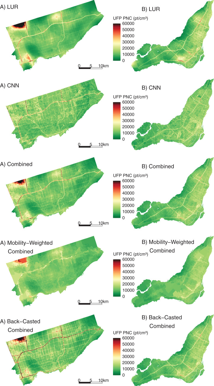
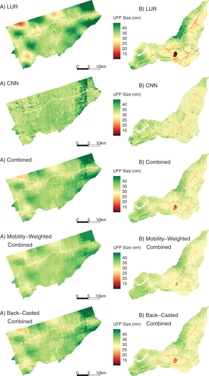
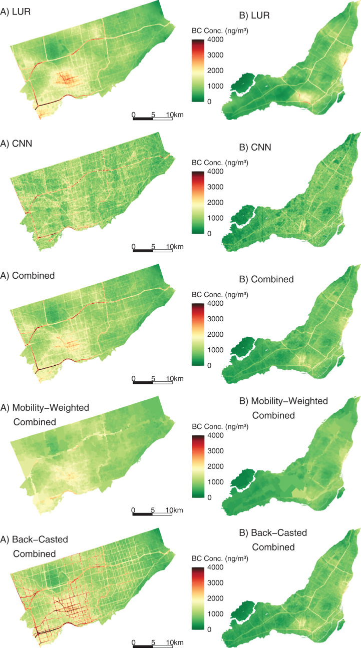
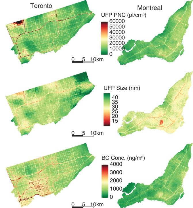
Figures 5, 6, and 7 show the predicted surfaces for outdoor UFP number concentrations (Figure 5), UFP Size (Figure 6), and BC (Figure 7) for the LUR, CNN, and combined models. Spatial variations in differences between LUR and CNN predictions are shown in Appendix Figures A.33–A.35 and show that for major highways, the Montreal CNN model consistently generated higher UFP number concentration predictions than did the LUR model, whereas for Toronto it was the opposite. LUR surfaces appeared more spatially smooth than CNN surfaces, but removing latitude and longitude from LUR models resulted in less spatial smoothing (Appendix Figures A.36–A.38) and reduced the elevated UFP number concentration predictions in northwestern Toronto. CNN model predictions using modified images were generally consistent with expectations (Appendix Figures A.39–A.42), though predictions appeared to be somewhat sensitive to the season in which images were captured (Appendix Figures A.43 and A.44).

Figure 7. — Exposure surfaces for predicted annual average outdoor BC (ng/m³) in Toronto (A) and Montreal (B) for the LUR, CNN, combined models, mobility-weighted combined models, and combined model backcasted to 2008. BC = black carbon; CNN = convolutional neural network; LUR = land use regression.

Mobility Weighting and Backcasting

Mobility-weighted surfaces are shown in Appendix Figures A.45–A.47. In general, mobility weighting increased lower predictions (i.e., if you live in a low-pollution area, leaving your house tends to increase your exposure) and decreased high predictions (i.e., if you live in a high-pollution area, leaving your house tends to decrease your exposure) for UFP number concentrations and BC (Appendix Figures A.48–A.51), which resulted in smoother surfaces. Historical traffic emissions were higher than contemporary levels, resulting in higher predicted concentrations in the backcasted surfaces, though less so for Montreal than for Toronto (Appendix Figures A.52, A.54, A.55, and A.57). Clear historical changes in the spatial distribution of UFP size were not apparent in our models (Appendix Figures A.53 and A.56).

Comparison of New UFP Models to Previous Models

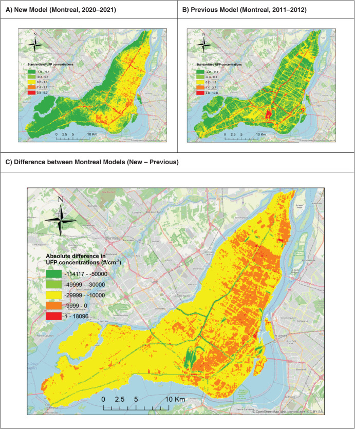
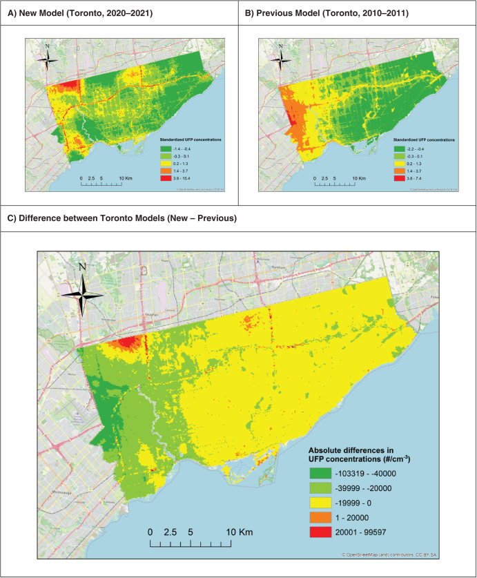
Comparisons of spatial variations in long-term average outdoor UFP number concentrations based on our new models and our previous models are shown in Table 5 and Figures 8 and 9. As expected, the focus of past campaigns on weekdays and rush-hour periods resulted in past models predicting higher concentrations than our new models, which captured all days of the week and most times of the day. Linear regression models comparing predictions from the new models to predictions from the old models had relatively low R² values (0.19 for Toronto and 0.18 for Montreal). Nevertheless, slopes of linear models relating the two models were reasonably high (0.70 for Toronto and 0.97 for Montreal), and the overall spatial patterns detected by both models were similar with elevated concentrations close to roadways and areas close to the airport in both cities. Although the aim of both the old and new models was to capture spatial variations in annual average outdoor UFP number concentrations, there were several important differences in how these models were developed that likely contributed to the low R² values. Specifically, the old models were trained using monitoring data collected only during weekday rush hour periods over a limited period of time (approximately 100 hours of monitoring), whereas the new models were trained using monitoring data from all days of the week and over a greater period of time (more than 500 hours of monitoring). Thus, although the models generally agree on areas of high and low concentrations (i.e., slope), there is variability in this agreement (i.e., low R²). Importantly, the new models were trained using monitoring data that is likely more representative of annual average outdoor UFP number concentrations than the monitoring data used to train the old models.

Figure 8. — Comparison of the new model for outdoor UFP number concentrations in Montreal (combined LUR-CNN model without backcasting or mobility weighting) with the previous model based on data collected in 2011–2012 on weekdays during rush-hour periods. Panels A and B show standardized concentrations, and panel C shows the spatial distribution of differences on the original scale. CNN = convolutional neural network; LUR = land use regression; UFP = ultrafine particles.

Figure 9. — Comparison of the new model for outdoor UFP number concentrations in Toronto (combined model without backcasting or mobility weighting) with the previous model based on data collected in 2010–2011 on weekdays during rush-hour periods. Panels A and B show standardized concentrations, and panel C shows the spatial distribution of differences on the original scale. UFP = ultrafine particles.

Table 5.

Mean Difference Between Outdoor UFP Number Concentrations Predicted from New Combined LUR-CNN Models and Previous Models for Toronto and Montreal^a

City	Mean Difference (95% CI)	Slope of Linear Model	Intercept of Linear Model	R ²
Toronto	−17,054 (−17,171, −16,938)	0.70	21,124	0.19
Montreal	−14,783 (−14,882, −14,683)	0.97	15,158	0.18

Open in a new tab

CI = confidence interval; CNN = convolutional neural network; LUR = land use regression; UFP = ultrafine particles.

^a Mean difference calculated as new model minus previous model. Previous models are described in references 12 and 13.

EPIDEMIOLOGICAL ANALYSIS

Our study population included 1,562,960 adults followed for a total of 22,848,100 person-years with 174,240 nonaccidental, 46,270 cardiovascular, 51,790 cardiometabolic, 26,570 ischemic heart disease, 9,310 cerebrovascular, 14,830 respiratory, and 16,790 lung cancer deaths occurring during the follow-up period. Descriptive statistics for cohort members are shown in Table 6, including mean standard deviation concentrations of outdoor air pollutants assigned at baseline (from our main combined backcasted model assigned to residential locations). At baseline, annual average outdoor UFP number concentrations ranged from approximately 3,200 to 162,000 particles/cm³, UFP size ranged from 18 to 50 nm, and BC ranged from 114 to 5,264 ng/m³. Mean outdoor PM_2.5 mass concentrations were 10.16 μg/m³ with a standard deviation of only 1.56 μg/m³; therefore, we do not present HRs for PM_2.5, as there was little within-city spatial variation. Correlations between outdoor air pollutants are shown in Table 7; UFP number concentrations were inversely correlated with UFP size (r = −0.54) and were weakly correlated with other air pollutants (0.10 <r <0.38). BC was moderately correlated with both PM_2.5 (r = 0.42) and O_x (r = 0.57).

Table 6.

Cohort Descriptive Statistics

	3-Year Mean (SD) Annual Residential Backcasted Exposure^a
	Person-Years^b	UFP Number (particles/cm³)	UFP Size (nm)	BC (ng/m³)	PM_2.5 (ug/m³)	O_x (ppb)
All
	22,848,100	13,982 (6,229)	33.22 (3.43)	1,109(552)	10.16 (1.56)	35.16 (3.66)
Sex
Female	12,324,900	13,994 (6,240)	33.22 (3.44)	1,111(554)	10.17 (1.54)	35.14 (3.63)
Male	10,523,200	13,968 (6,217)	33.23 (3.43)	1,107(550)	10.14 (1.58)	35.17 (3.68)
Age group (years)
25 to 29	2,237,100	14,337 (6,334)	33.15 (3.36)	1,139(567)	10.07 (1.62)	35.23 (3.87)
30 to 39	5,572,300	14,069 (6,351)	33.28 (3.39)	1,125(560)	10.11 (1.61)	35.28 (3.73)
40 to 49	5,600,400	13,828 (6,172)	33.30 (3.45)	1,095(543)	10.17 (1.55)	35.18 (3.61)
50 to 59	4,188,800	13,864 (6,299)	33.21 (3.47)	1,090(543)	10.19 (1.52)	35.09 (3.59)
60 to 69	3,063,500	13,961 (6,192)	33.14 (3.48)	1,096(542)	10.23 (1.54)	35.07 (3.58)
70 to 79	1,768,100	13,979 (5,923)	33.13 (3.43)	1,117(556)	10.22 (1.50)	34.98 (3.54)
80 to 89	417,800	14,094 (5,950)	33.12 (3.37)	1,148(576)	10.10 (1.43)	34.77 (3.44)
Visible minority status
White or Aboriginal	16,954,300	13,705 (5,792)	33.05 (3.41)	1,081(542)	10.11 (1.65)	34.78 (3.67)
Visible minority	5,893,700	14,779 (7,288)	33.72 (3.44)	1,189(572)	10.29 (1.24)	36.27 (3.39)
Immigrant status
Nonimmigrant	12,172,200	13,664 (5,404)	32.86 (3.42)	1,033(503)	9.97 (1.72)	34.37 (3.64)
Immigrant	10,675,800	14,341 (7,030)	33.63 (3.40)	1,195(591)	10.39 (1.30)	36.12 (3.43)
Marital status
Single	4,550,000	14,610 (6,118)	32.91 (3.33)	1,152(576)	10.25 (1.53)	35.15 (3.76)
Common law	1,862,500	13,889 (5,089)	32.46 (3.34)	1,004(496)	9.71 (1.79)	33.82 (3.66)
Married	13,043,500	13,662 (6,409)	33.50 (3.45)	1,098(540)	10.18 (1.53)	35.40 (3.57)
Separated	664,200	14,624 (6,586)	33.29 (3.47)	1,201(603)	10.29 (1.53)	35.52 (3.69)
Divorced	1,536,500	14,514 (6,163)	32.79 (3.41)	1,134(580)	10.17 (1.57)	34.88 (3.69)
Widowed	1,191,300	14,121 (5,922)	33.08 (3.46)	1,136(571)	10.26 (1.48)	35.06 (3.55)
Education attainment
Not completed high school	5,766,200	14,174 (6,389)	33.10 (3.48)	1,127(565)	10.35 (1.49)	35.37 (3.67)
High school with or without trades certificate	6,903,900	13,973 (6,379)	33.17 (3.53)	1,087(542)	10.11 (1.57)	35.08 (3.66)
Postsecondary nonuniversity	4,149,000	13,876 (6,269)	33.31 (3.47)	1,091(548)	10.01 (1.61)	35.04 (3.65)
University degree	6,029,000	13,865 (5,835)	33.34 (3.23)	1,130(551)	10.14 (1.55)	35.12 (3.63)
Occupational level
Management	1,947,900	13,525 (6,097)	33.38 (3.28)	1,089(548)	10.08 (1.65)	35.14 (3.68)
Professional	3,661,100	13,683 (5,641)	33.35 (3.28)	1,110(538)	10.13 (1.59)	35.08 (3.66)
Skilled, technical, supervisory	4,209,800	13,814 (6,301)	33.30 (3.48)	1,094(547)	10.09 (1.60)	35.16 (3.68)
Semiskilled	4,959,500	14,166 (6,676)	33.26 (3.52)	1,112(555)	10.16 (1.53)	35.33 (3.65)
Unskilled	1,607,300	14,411 (6,546)	33.24 (3.49)	1,174(591)	10.29 (1.49)	35.49 (3.70)
Not applicable	6,462,500	14,126 (6,087)	33.04 (3.43)	1,107(550)	10.20 (1.53)	34.99 (3.61)
Income adequacy quintile
1st quintile (lowest)	4,918,000	14,735 (6,423)	33.04 (3.38)	1,177(587)	10.29 (1.48)	35.37 (3.70)
2nd quintile	4,689,800	14,198 (6,446)	33.22 (3.48)	1,131(563)	10.22 (1.49)	35.33 (3.63)
3rd quintile	4,459,400	13,883 (6,344)	33.28 (3.52)	1,096(544)	10.14 (1.54)	35.18 (3.64)
4th quintile	4,220,500	13,587 (6,112)	33.31 (3.50)	1,068(526)	10.07 (1.59)	35.05 (3.65)
5th quintile (highest)	4,560,400	13,334 (5,611)	33.29 (3.28)	1,058(518)	10.05 (1.70)	34.80 (3.63)

Open in a new tab

BC = black carbon; SD = standard deviation; O_x = oxidant gases; PM_2.5 = particulate matter ≤2.5 μm in aerodynamic diameter; UFP = ultrafine particles.

^aAll columns showing mean (sd) are the exposure values at cohort entry.

^bThe person-years column was rounded to the nearest 100 for confidentiality.

Table 7.

Correlations Between Air Pollutants Assigned at Baseline (Combined LUR-CNN Backcasted)

	UFP Number	UFP Size	BC	O_x	PM_2.5
UFP Number	1
UFP Size	−0.54	1
BC	0.38	0.09	1
O_x	0.17	0.22	0.57	1
PM_2.5	0.10	0.17	0.42	0.51	1

Open in a new tab

BC = black carbon; O_x = oxidant gases; PM_2.5 = particulate matter ≤2.5 μm in aerodynamic diameter; UFP = ultrafine particles.

Main Analysis (Based on Combined LUR-CNN Models with Backcasting)

Hazard ratios describing associations observed between outdoor UFP number concentrations, BC, and mortality are shown in Table 8. Outdoor UFP number concentrations (scaled per 10,000 particles/cm³) were positively associated with all mortality outcomes with the strongest association observed for respiratory (HR = 1.174, 95% CI = 1.130, 1.220) and ischemic heart disease mortality (HR = 1.094, 95% CI: 1.062, 1.126). BC was not associated with increased risks of respiratory or lung cancer mortality, but small positive associations were observed for the other mortality outcomes. HRs for BC decreased with the inclusion of other air pollutants in the models, likely owing to the moderate correlation between BC and O_x along with the positive association of O_x with all mortality outcomes except lung cancer (Appendix Table A.16). HRs for UFP number concentrations increased in multipollutant models owing to negative confounding by UFP size, which is discussed below.

Table 8.

Hazard Ratios for Long-Term Exposures to Outdoor UFP Number Concentrations, BC, and Mortality^a

Cause of Mortality	Hazard Ratio (95% CI)
Cause of Mortality	UFP Number (per 10,000 particles/cm³)	BC (per 500 ng/m³)
Nonaccidental	1.073 (1.061, 1.085)	1.009 (1.004, 1.015)
Cardiovascular	1.069 (1.047, 1.094)	1.015 (1.004, 1.027)
Cardiometabolic	1.075 (1.052, 1.098)	1.015 (1.004, 1.025)
Ischemic heart disease	1.094 (1.062, 1.126)	1.009 (0.995, 1.025)
Cerebrovascular	1.061 (1.007, 1.117)	1.025 (0.999, 1.052)
Respiratory	1.174 (1.130, 1.220)	0.979 (0.959, 0.999)
Lung cancer	1.057 (1.017, 1.098)	0.987 (0.967, 1.008)

Open in a new tab

BC = black carbon; CI = confidence interval; UFP = ultrafine particles.

^aAll models included sociodemographic variables, PM_2.5, O_x, UFP size, and either BC or UFP number concentrations.

Table 9 shows the HRs for outdoor UFP number concentrations with and without adjusting for mean UFP size using a linear or spline term. For all mortality outcomes except lung cancer, HRs were considerably lower when UFP size was not included in the model. This was particularly true for cerebrovascular mortality where confounding by UFP size (i.e., not adjusting for UFP size) resulted in a null association with outdoor UFP number concentrations. UFP number concentrations and UFP size were each considered as potential risk factors for mortality; thus, they were included in multipollutant models in the main analysis for BC. HRs for BC and mortality are shown in Table 10 with and without adjustment for UFP size. In this case, adjusting for UFP size decreased HRs for BC only slightly, with weaker associations observed between BC and nonaccidental, cardiometabolic, cardiovascular, ischemic heart disease, and cerebrovascular mortality after adjustment for UFP size. Table 11 compares the HRs of single-pollutant models to the HRs of the main analysis that included co-pollutants (i.e., multipollutant models). In single-pollutant models, UFP number concentrations were associated with all mortality outcomes except cerebrovascular mortality, and adjusting for co-pollutants resulted in these associations becoming stronger, which included an association with cerebrovascular mortality. BC mass concentrations were associated with all mortality outcomes except lung cancer, but when adjusting for co-pollutants, the associations became weaker, with ischemic heart disease, cerebrovascular, and respiratory mortality becoming null in the multipollutant models.

Table 9.

Hazard Ratios for Outdoor UFP Number Concentrations (per 10,000 particles/cm³) and Mortality with and without Controlling for UFP Size^a

Cause of Mortality	Hazard Ratio for UFP Number (95% CI)
Cause of Mortality	No Adjustment for UFP Size	Linear Adjustment for UFP Size	Nonlinear Adjustment for UFP Size (main analysis)
Nonaccidental	1.034 (1.024, 1.043)	1.052 (1.040, 1.064)	1.073 (1.061, 1.085)
Cardiovascular	1.017 (1.002, 1.034)	1.055 (1.033, 1.076)	1.069 (1.047, 1.094)
Cardiometabolic	1.022 (1.007, 1.040)	1.061 (1.040, 1.082)	1.075 (1.052, 1.098)
Ischemic heart disease	1.022 (1.000, 1.045)	1.082 (1.052, 1.110)	1.094 (1.062, 1.126)
Cerebrovascular	0.986 (0.949, 1.026)	1.041 (0.991, 1.092)	1.061 (1.007, 1.117)
Respiratory	1.092 (1.061, 1.123)	1.143 (1.105, 1.185)	1.174 (1.130, 1.220)
Lung cancer	1.054 (1.026, 1.084)	1.040 (1.002, 1.078)	1.057 (1.017, 1.098)

Open in a new tab

CI = confidence interval; UFP = ultrafine particles.

^aAll models included sociodemographic variables, PM_2.5, O_x, and BC.

Table 10.

Hazard Ratios for BC (per 500 ng/m³) and Mortality with and without Controlling for UFP Size^a

Cause of Mortality	Hazard Ratios for BC (95% CI)
Cause of Mortality	No Adjustment for UFP Size	Linear Adjustment for UFP Size	Nonlinear Adjustment for UFP Size (main analysis)
Nonaccidental	1.018 (1.012, 1.024)	1.015 (1.008, 1.020)	1.009 (1.004, 1.015)
Cardiovascular	1.025 (1.015, 1.037)	1.019 (1.007, 1.030)	1.015 (1.004, 1.027)
Cardiometabolic	1.025 (1.015, 1.035)	1.018 (1.007, 1.029)	1.015 (1.004, 1.025)
Ischemic heart disease	1.023 (1.008, 1.037)	1.012 (0.996, 1.026)	1.009 (0.995, 1.025)
Cerebrovascular	1.041 (1.016, 1.067)	1.031 (1.005, 1.057)	1.025 (0.999, 1.052)
Respiratory	0.995 (0.975, 1.015)	0.985 (0.965, 1.005)	0.979 (0.959, 0.999)
Lung cancer	0.988 (0.969, 1.007)	0.991 (0.971, 1.011)	0.987 (0.967, 1.008)

Open in a new tab

BC = black carbon; CI = confidence interval; UFP = ultrafine particles.

^aAll models included sociodemographic variables, PM_2.5, O_x, and UFP number concentrations.

Table 11.

Hazard Ratios for Outdoor UFP Number Concentrations, BC, and Mortality in Single-Pollutant Models Using the Main Combined LUR-CNN Exposure Model^a

Cause of Mortality	Hazard Ratio (95% CI)
	UFP Number (per 10,000 particles/cm³)		BC (per 500 ng/m³)
	Single-Pollutant Model	Multipollutant Model	Single-Pollutant Model	Multipollutant Model
Nonaccidental	1.050 (1.041, 1.057)	1.073 (1.061, 1.085)	1.031 (1.026, 1.035)	1.009 (1.004, 1.015)
Cardiovascular	1.043 (1.028, 1.059)	1.069 (1.047, 1.094)	1.044 (1.035, 1.053)	1.015 (1.004, 1.027)
Cardiometabolic	1.047 (1.033, 1.062)	1.075 (1.052, 1.098)	1.044 (1.035, 1.052)	1.015 (1.004, 1.025)
Ischemic heart disease	1.050 (1.029, 1.073)	1.094 (1.062, 1.126)	1.052 (1.040, 1.063)	1.009 (0.995, 1.025)
Cerebrovascular	1.021 (0.986, 1.057)	1.061 (1.007, 1.117)	1.046 (1.027, 1.066)	1.025 (0.999, 1.052)
Respiratory	1.100 (1.069, 1.128)	1.174 (1.130, 1.22)	1.034 (1.019, 1.051)	0.979 (0.959, 0.999)
Lung cancer	1.041 (1.015, 1.069)	1.057 (1.017, 1.098)	0.989 (0.974, 1.004)	0.987 (0.967, 1.008)

Open in a new tab

BC = black carbon; CI = confidence interval; UFP = ultrafine particles.

^aAll single-pollutant models are adjusted for sociodemographic variables. The main multipollutant models are shown for comparison and adjusted for sociodemographic variables, PM_2.5, O_x, UFP size, and either BC or UFP number concentrations.

Concentration-response relationships between outdoor UFP number concentrations, UFP size, and mortality outcomes are shown in Figures 10 and 11 along with the joint distribution of UFP size and UFP number concentrations. For nonaccidental mortality, the concentration-response curve for UFP number concentrations flattens and decreases at elevated UFP levels (above 22,500 particles/cm³), whereas the concentration-response curve for UFP size increases continuously as UFP size increases from approximately 10 nm to 40 nm. As shown in the I panels of Figures 10 and 11, the distribution of UFP size was heterogeneous across the range of UFP number concentrations, with a lower proportion of the larger UFPs (i.e., those most strongly associated with mortality) present at higher UFP number concentrations. This likely explains the observed decrease in the concentration-response curve observed at higher number concentrations in the A panels of Figures 10 and 11 (i.e., the curve for UFP number concentrations needs to decrease at higher concentrations to reflect the fact that the size of particles present at this concentration is not as strongly associated with mortality). A similar pattern was observed for other mortality outcomes, with the possible exception of lung cancer where the concentration-response curve for UFP size peaked around approximately 30 nm and then flattened off. However, the concentration-response curve for UFP number concentrations and lung cancer remained consistent with the observed distribution of UFP size across the number concentration range (i.e., a lower proportion of the particles sizes more strongly associated with mortality at elevated UFP number concentrations). Concentration-response curves for BC are shown in Appendix Figure A.58. For nonaccidental, cardiovascular, cardiometabolic, and ischemic heart disease mortality, a threshold-type shape was apparent, but HRs then decreased at higher concentrations. Concentration-response curves for outdoor UFP number concentrations and UFP size from LUR and CNN models separately and mortality outcomes are shown in Appendix Figure A.59. The shapes of the curves were generally similar to those of the combined models (Figure 10), however, the curve flattening at elevated UFP number concentrations was less pronounced for the CNN models than it was for the LUR models.

Figure 10. — Concentration-response curves for outdoor UFP number concentrations; UFP size; and nonaccidental, cardiovascular, respiratory, and lung cancer mortality along with frequency plots of joint exposures to UFP number concentration and UFP size. Curves were fit using penalized splines with generalized cross-validation to select the optimal smoothness parameters. UFP = ultrafine particles.

Figure 11. — Concentration-response curves for outdoor UFP number concentrations; UFP size; and cardiometabolic, cerebrovascular, and ischemic heart disease mortality along with frequency plots of joint exposures to UFP number concentration and UFP size. Curves were fit using penalized splines with generalized cross-validation to select the optimal smoothness parameters. UFP = ultrafine particles.

Sensitivity of Epidemiological Results to Backcasting, Mobility Weighting, and Exposure Model Type

Analyses examining the sensitivity of HRs from our main exposure models (i.e., combined LUR-CNN model) to backcasting and mobility weighting are shown in Tables 12 and 13 for UFP number concentrations and BC, respectively. In general, backcasting had little impact on observed HRs for UFP number concentrations or BC; however, for BC, backcasting did change the direction of association for nonaccidental, cardiovascular, and cardiometabolic (i.e., from slightly inverse to slightly positive) mortality outcomes. HRs based on mobility-weighted UFP exposures tended to be lower but generally remained positively associated with all mortality outcomes. This pattern may have occurred because mobility weighting was not conducted at the individual level, and thus the mobility-weighted models may contribute exposure measurement error to the epidemiological analyses. Associations between BC and mortality remained mostly null (or very weak) when mobility-weighted exposures were used, although HRs for lung cancer and respiratory mortality strengthened slightly in the inverse direction.

Table 12.

Hazard Ratios per 10,000 particles/cm³ Increase in UFP Number Concentrations and Mortality from Combined LUR-CNN Model (Main Exposure Model) with and without Backcasting and with and without Mobility Weighting^a

Cause of Mortality	Backcasted HR (95% CI)		Mobility Weighted HR (95% CI)
Cause of Mortality	Yes (main analysis)	No	Backcasted	Not Backcasted
Nonaccidental	1.073 (1.061, 1.085)	1.078 (1.064, 1.094)	1.034 (1.019, 1.046)	1.053 (1.035, 1.072)
Cardiovascular	1.069 (1.047, 1.094)	1.072 (1.043, 1.100)	1.057 (1.029, 1.085)	1.069 (1.035, 1.106)
Cardiometabolic	1.075 (1.052, 1.098)	1.080 (1.054, 1.108)	1.066 (1.038, 1.091)	1.081 (1.047, 1.113)
Ischemic heart disease	1.094 (1.062, 1.126)	1.102 (1.066, 1.141)	1.076 (1.042, 1.113)	1.106 (1.060, 1.153)
Cerebrovascular	1.061 (1.007, 1.117)	1.045 (0.983, 1.110)	1.046 (0.986, 1.111)	1.035 (0.959, 1.118)
Respiratory	1.174 (1.130, 1.220)	1.201 (1.149, 1.256)	1.124 (1.074, 1.176)	1.184 (1.120, 1.253)
Lung cancer	1.057 (1.017, 1.098)	1.074 (1.027, 1.122)	1.021 (0.975, 1.070)	1.053 (0.998, 1.115)

Open in a new tab

CI = confidence interval; HR = hazard ratio.

^aAll models included sociodemographic variables, PM_2.5, O_x, UFP size, and BC.

Table 13.

Hazard Ratios per 500 ng/m³ Increase in BC and Mortality from Combined LUR-CNN Model (Main Exposure Model) with and without Backcasting and with and without Mobility Weighting^a

Cause of Mortality	Backcasted HR (95% CI)		Mobility-Weighted HR (95% CI)
Cause of Mortality	Yes (main analysis)	No	Backcasted	Not Backcasted
Nonaccidental	1.009 (1.004, 1.015)	0.994 (0.985, 1.002)	1.000 (0.991, 1.009)	0.975 (0.965, 0.986)
Cardiovascular	1.015 (1.004, 1.027)	0.999 (0.984, 1.017)	1.007 (0.991, 1.024)	0.988 (0.968, 1.008)
Cardiometabolic	1.015 (1.004, 1.025)	0.999 (0.984, 1.015)	1.006 (0.991, 1.022)	0.986 (0.967, 1.006)
Ischemic heart disease	1.009 (0.995, 1.025)	0.993 (0.972, 1.015)	1.002 (0.981, 1.024)	0.980 (0.954, 1.007)
Cerebrovascular	1.025 (0.999, 1.052)	1.004 (0.967, 1.040)	1.032 (0.995, 1.070)	1.012 (0.967, 1.059)
Respiratory	0.979 (0.959, 0.999)	0.946 (0.918, 0.974)	0.968 (0.940, 0.997)	0.920 (0.886, 0.953)
Lung cancer	0.987 (0.967, 1.008)	0.981 (0.953, 1.009)	0.952 (0.925, 0.981)	0.945 (0.913, 0.979)

Open in a new tab

CI = confidence interval; HR = hazard ratio.

^aAll models included sociodemographic variables, PM_2.5, O_x, UFP number concentrations, and UFP size.

Mortality HRs from the LUR and CNN models separately (as opposed to their combined use in our main exposure model) are shown in Tables 14 and 15 for UFP number concentrations and BC, respectively. In general, stronger associations were observed between UFP number concentrations and mortality for analyses based on the CNN model alone compared to the LUR model alone. In most cases, differences were small, with larger differences observed for nonaccidental mortality, respiratory mortality, and lung cancer mortality. For BC, results were similar for both modeling approaches, with HRs close to the null (sometimes slightly above the null and sometimes slightly below the null). For respiratory and lung cancer mortality, inverse associations with BC were stronger in analyses using the CNN model compared to using the LUR model.

Table 14.

Hazard Ratios for 10,000 particles/cm³ Increase in UFP Number Concentrations and Mortality from the LUR and CNN Models Separately with and Without Backcasting and with and Without Mobility Weighting^a

Cause of Mortality	Backcasted HR (95% CI)		Mobility-Weighted HR (95% CI)
Cause of Mortality	Yes	No	Backcasted	Not Backcasted
LUR Model
Nonaccidental	1.028 (1.021, 1.037)	1.025 (1.017, 1.035)	1.012 (1.003, 1.021)	1.017 (1.006, 1.028)
Cardiovascular	1.037 (1.023, 1.053)	1.034 (1.017, 1.052)	1.033 (1.017, 1.050)	1.036 (1.015, 1.059)
Cardiometabolic	1.040 (1.027, 1.054)	1.039 (1.023, 1.056)	1.040 (1.024, 1.057)	1.043 (1.024, 1.065)
Ischemic heart disease	1.051 (1.033, 1.07)	1.052 (1.030, 1.074)	1.047 (1.026, 1.069)	1.059 (1.032, 1.086)
Cerebrovascular	1.041 (1.007, 1.075)	1.023 (0.985, 1.064)	1.033 (0.993, 1.071)	1.021 (0.972, 1.070)
Respiratory	1.068 (1.043, 1.094)	1.073 (1.042, 1.104)	1.052 (1.022, 1.082)	1.068 (1.032, 1.107)
Lung cancer	1.013 (0.987, 1.037)	1.015 (0.987, 1.044)	0.993 (0.964, 1.022)	1.004 (0.968, 1.042)
CNN Model
Nonaccidental	–	1.114 (1.097, 1.132)	–	1.101 (1.075, 1.125)
Cardiovascular	–	1.050 (1.019, 1.084)	–	1.026 (0.978, 1.075)
Cardiometabolic	–	1.060 (1.029, 1.092)	–	1.026 (0.984, 1.071)
Ischemic heart disease	–	1.053 (1.009, 1.097)	–	1.010 (0.950, 1.071)
Cerebrovascular	–	1.021 (0.951, 1.097)	–	0.975 (0.879, 1.081)
Respiratory	–	1.265 (1.199, 1.337)	–	1.283 (1.185, 1.387)
Lung cancer	–	1.160 (1.102, 1.223)	–	1.206 (1.118, 1.302)

Open in a new tab

CI = confidence interval; CNN = convolutional neural network; HR = hazard ratio; LUR = land use regression.

^aAll models included sociodemographic variables, PM_2.5, O_x, UFP size, and BC.

Table 15.

Hazard Ratios for 500 ng/m³ Increase in BC and Mortality from the LUR and CNN Models Separately with and without Backcasting and with and without Mobility Weighting^a

Cause of Mortality	Backcasted HR (95% CI)		Mobility-Weighted HR (95% CI)
Cause of Mortality	Yes	No	Backcasted	Not Backcasted
LUR Model
Nonaccidental	1.016 (1.012, 1.022)	1.006 (0.999, 1.013)	1.007 (1.000, 1.014)	0.989 (0.981, 0.999)
Cardiovascular	1.017 (1.008, 1.027)	1.005 (0.991, 1.018)	1.009 (0.996, 1.023)	0.995 (0.978, 1.012)
Cardiometabolic	1.018 (1.009, 1.026)	1.006 (0.993, 1.019)	1.008 (0.996, 1.021)	0.993 (0.977, 1.009)
Ischemic heart disease	1.011 (0.999, 1.023)	0.996 (0.978, 1.014)	1.003 (0.985, 1.021)	0.986 (0.964, 1.008)
Cerebrovascular	1.028 (1.007, 1.049)	1.016 (0.986, 1.049)	1.029 (0.999, 1.059)	1.015 (0.977, 1.054)
Respiratory	1.001 (0.985, 1.018)	0.978 (0.954, 1.002)	0.989 (0.966, 1.012)	0.951 (0.922, 0.979)
Lung cancer	0.999 (0.983, 1.016)	0.996 (0.974, 1.020)	0.976 (0.953, 0.998)	0.977 (0.950, 1.005)
CNN Model
Nonaccidental	–	0.983 (0.973, 0.993)	–	0.975 (0.960, 0.989)
Cardiovascular	–	1.001 (0.983, 1.020)	–	1.021 (0.994, 1.050)
Cardiometabolic	–	1.000 (0.982, 1.017)	–	1.024 (0.997, 1.051)
Ischemic heart disease	–	1.014 (0.990, 1.038)	–	1.043 (1.006, 1.082)
Cerebrovascular	–	0.976 (0.937, 1.017)	–	1.030 (0.968, 1.096)
Respiratory	–	0.937 (0.909, 0.969)	–	0.926 (0.883, 0.973)
Lung cancer	–	0.986 (0.957, 1.018)	–	0.918 (0.876, 0.962)

Open in a new tab

CI = confidence interval; CNN = convolutional neural network; HR = hazard ratio; LUR = land use regression.

^aAll models included sociodemographic variables, PM_2.5, O_x, UFP number concentrations, and UFP size.

DISCUSSION AND CONCLUSIONS

EXPOSURE MODEL DEVELOPMENT AND EVALUATION

In this study, we developed new high-resolution exposure models to predict within-city spatial variations in outdoor UFP number concentrations, mean UFP size, and BC mass concentrations for Canada’s two largest cities. This analysis improves on our earlier models^12,13 by increasing the spatial coverage of the monitoring campaign, increasing the total monitoring time, extending the monitoring period over an entire year, randomly sampling all days of the week and most times of day, and incorporating information from digital aerial images into model predictions using CNNs. The increased spatial and temporal coverage of this monitoring campaign compared to our previous effort likely resulted in a more representative sample of the within-city spatial variations of annual average outdoor air pollution. Model R² values cannot be directly compared across studies, but the R² values of our LUR, CNN, and combined models fell within the range of published R² values from other studies that developed LUR models, machine learning models, or CNN models trained on images of the urban environment.^{12,13,22,43,53–55} The magnitude of the bias observed in our models was similar to the bias reported by other studies as well.^12,43,53,55 A further improvement over our earlier models was the development of models for mean UFP size, which generally predicted smaller mean UFP sizes in areas of elevated UFP number concentrations, which is consistent with other research⁵⁶ and our understanding of particle growth (i.e. fresh emissions consisting of high concentrations of very small particles).^57,58 The development of mean UFP size models is important because particle size may play a role in UFP toxicity^59–61 and has the potential to confound associations between outdoor UFP number concentrations and adverse health outcomes, as discussed previously. Collectively, this investigation produced a number of interesting results.

First, we observed high within-city spatial variations in outdoor UFP number concentrations, mean UFP size, and BC concentrations during mobile monitoring, all of which were monitored and modeled on the same spatial and temporal scales following the same methods. This finding is consistent with those from other studies that reported outdoor UFP and BC concentrations as having much greater within-city spatial variations than outdoor PM_2.5 concentrations.^22,62–64 The high-resolution models we developed explained more than half of the observed spatial variation in outdoor UFP and BC concentrations in the test sets. Our predicted UFP number concentrations were less strongly correlated with other air pollutants (PM_2.5 r = 0.10, BC r = 0.38) than other models recently developed for Southern California (PM_2.5 r = 0.28, BC r = 0.64).²² City-specific models performed better than multicity models trained on pooled data, which is consistent with the documented difficulty of transferring models between study areas.^65–67 The CNN models performed somewhat worse than the LUR models but took advantage of an alternative data stream (i.e., images instead of GIS data), and it is possible that the CNN models learned complex associations that were not present in GIS data alone. Combined models performed better than any LUR or CNN models on their own, though with only a modest increase in R² compared to the LUR models. This is consistent with the results from a similar study⁴³ and suggests that CNNs trained on images can be useful for predicting within-city spatial variations in outdoor air pollution, especially when combined with LUR models. Nonetheless, CNNs can learn unintended associations between image features and underlying structures in the data, which can affect generalizability.^68–70 For example, our CNNs appeared to be somewhat sensitive to the time of year images were captured, which likely introduced measurement error into our estimates. Nevertheless, our results suggest that CNN models are useful in capturing spatial information on environmental exposures, and this may be particularly useful in places lacking large, curated databases of land use and traffic information, as recently demonstrated in Bucaramanga, Colombia.⁴³

Second, for each pollutant, the LUR and CNN models generated similar prediction surfaces, yet there were several interesting differences. For instance, the LUR model prediction surfaces were generally smoother than those from CNN models. This difference was due in part to the inclusion of latitude and longitude in the LUR models. Latitude and longitude vary incrementally throughout the study area and smoothed the LUR predictions, whereas each CNN-generated prediction was based solely on digital images that covered up to 280 m × 280 m of the earth’s surface (i.e., the CNN prediction for a given point was naïve to any information beyond the edge of the image centered on that point). UFP and BC concentrations can vary greatly over very short distances,^4,62,63 and it is possible LURs may have over-smoothed the spatial variations in certain areas. In other areas, however, the CNN may have resulted in under-smoothing, as it is naïve to information beyond the limits of the images. Combined model prediction surfaces appeared to integrate the smoothness of the LUR surfaces with the sharp gradients of the CNN surfaces, which may be a useful compromise between the two approaches. Furthermore, mapping the difference between LUR and CNN model predictions highlighted interesting contrasts. For example, on major highways, the Montreal LUR model consistently predicted higher UFP number concentrations than the Montreal CNN model, whereas in Toronto, it was the opposite. In general, combining LUR and CNN predictions resulted in only a modest increase in overall model performance compared to the LUR models alone, but the combined models may help generate more robust predictions throughout the modeling areas by taking advantage of information from both land use data and digital images. In our previous study, conducted in Colombia, spatial variations in model errors were lower for CNN models than for LUR models.⁴³

A strength of our exposure modeling study was the large scope of the monitoring campaign, and mobile monitoring was an efficient approach to maximize spatial coverage, though a limitation was relatively low monitoring time per road segment compared to stationary monitoring.^55,71 On average, road segments were visited on 10 different days for a total of roughly 60 seconds of monitoring. Although researchers have successfully developed models based on similar levels of monitoring,^12,13,71,72 longer monitoring times would likely provide more stable estimates of annual average ambient UFP and BC levels. In addition, mobile monitoring was conducted using internal combustion engine vehicles driving on roads and major highways, which likely resulted in our measured values of air pollution being higher than the air pollution values immediately outside residences. However, it is important to note that many areas were detected with low air pollution levels, and thus our use of gasoline vehicles did not prevent us from capturing a wide range of pollutant concentrations across each city. Nevertheless, future monitoring campaigns could follow the approach recently used by Blanco and colleagues to address this limitation (i.e., building in stopping locations along each route).⁷³

Another strength of this study was the incorporation of information from digital images to improve predictions. However, the application of CNNs can be challenging. First, CNNs require a large amount of training data and may not be applicable for smaller monitoring campaigns. Second, CNNs do not have the easily interpretable coefficients of linear regression models; however, we explored several approaches to verify that CNN models responded in a logical manner, and results were generally consistent with our current understanding of UFP sources (e.g., adding a road to an image of green space generally increased model predictions). Third, quality control of digital images is an extremely important and potentially resource-intensive step^74,75 when training CNN models. For example, past applications of CNNs have erroneously learned structural flaws in the data when training models on images from multiple databases.^76,77 Using R to download Google Maps satellite images was an efficient approach to compile a high-quality database of digital images, but we could not control the exact timing of image capture. This led to some images being from different seasons during the year-long campaign and likely had a small impact on CNN model predictions. Future studies should consider allocating resources to establishing high-quality databases of digital images for CNN model training and possibly developing methods to take advantage of seasonal differences in digital images to generate robust estimates of spatial variations in air pollution.

EPIDEMIOLOGICAL ANALYSIS

In the cohort study portion of this project, we followed a large population of adults in Montreal and Toronto and found consistent positive associations between long-term exposure to outdoor UFP number concentrations and both nonaccidental and cause-specific mortality. These associations were independent of other outdoor air pollutants, including PM_2.5 and oxidant gases. The associations persisted when using different exposure models and, importantly, also adjusted for UFP size (i.e., mean UFP diameter), which has not been done in previous studies and could result in an underestimation of health risks when excluded from the analyses. Results for BC were largely null, although small positive associations were observed for some mortality outcomes.

As noted earlier, few cohort studies have examined the relationship between long-term exposure to outdoor UFP number concentrations and mortality. A study in California reported a positive association between outdoor UFPs and ischemic heart disease mortality,²³ but exposures were estimated at a spatial resolution of approximately 4 km, which is too coarse to capture fine-scale spatial variations that may affect health. Similarly, Pond and colleagues¹⁶ reported positive associations between UFPs and nonaccidental and cause-specific mortality, but results were sensitive to the inclusion of PM_2.5 in models. In addition, this study aggregated UFP exposures to the census tract level, which likely contributed substantially to exposure measurement error for UFPs (more so than for PM_2.5), making it difficult to directly compare the results of this study to those using high-resolution exposure information. More recently, a cohort study in the Netherlands reported positive associations between outdoor UFP number concentrations and mortality using high-resolution estimates of spatial variations in long-term average outdoor UFP concentrations.¹⁵ Although this study did not adjust for UFP size, the observed associations (nonaccidental HR = 1.045, 95% CI: 1.037, 1.056; respiratory HR = 1.083, 95% CI: 1.049, 1.123; rescaled to match 10,000 particles/cm³ increment used in this study) were similar in magnitude to those observed in the present study (when expressed on the same scale) when we excluded UFP size from our models (nonaccidental HR = 1.034, 95% CI: 1.024, 1.043; respiratory HR = 1.092, 95% CI: 1.061, 1.123). Other studies of long-term exposures to UFPs and mortality were not identified, but studies in Denmark have compared the health risks of total outdoor UFP number concentrations as well as traffic-related UFP number concentrations.^78,79

Specifically, in these studies, traffic-related UFPs were more strongly associated with type 2 diabetes incidence⁸⁰ with weaker associations observed for incident myocardial infarctions.⁸¹ More generally, these previous observations and our results with respect to confounding by UFP size highlight the fact that we should not treat all UFP number concentrations as though they reflect a single type of exposure. This relates more broadly to the issue of confounding of version of treatment-outcome associations when studying exposures with multiple versions of treatment, which is likely an underappreciated source of bias in air pollution epidemiology for pollutants that have historically been treated as a single entity (e.g., UFP number concentrations or PM_2.5 mass concentrations) but in reality represent a complex mixture of component parts with varying levels of toxicity.²⁴ In the context of our results, it is clear that for outdoor UFP number concentrations, we need to consider UFP size because the size distribution of UFPs varies across the range of outdoor UFP number concentrations and UFP size is independently associated with mortality. Importantly, our results suggest that failure to consider UFP size in the analysis may result in an underestimation of the health effects of outdoor UFP number concentrations. In our analysis HRs were approximately four times smaller for cardiovascular mortality and disappeared altogether for cerebrovascular mortality when UFP size was excluded from the models. As such, UFP size should be considered in epidemiological analyses to avoid the potential bias in health risk estimates for UFP number concentrations. This is consistent with a recent review by Kittelson and colleagues that recommended using UFP number, mass, and surface area (i.e., size) to properly characterize UFP exposures.⁵⁷ In the same manner that earlier toxicological research investigated the varying health effects of different number concentrations by holding mass concentration constant,^82,83 future investigations into the health effects of UFP number concentrations should control for potential variations in UFP size.

In general, our results for UFPs were robust to sensitivity analyses both with and without backcasting and with and without mobility weighting, although mobility-weighted results were attenuated. This is likely attributable to mobility weighting being conducted at the neighborhood level as opposed to the individual level, and thus the mobility-weighting process likely contributed to exposure measurement error at the individual level. In addition, the results of epidemiological analyses for UFPs conducted separately for the LUR and CNN models generally suggested stronger associations for CNN model estimates. The reasons for this are unclear but may be related to the issue of spatial smoothing whereby the CNN model exposures are more local in nature; in contrast, LUR models exhibit more spatial smoothing owing to the nature of the variables included in the model. If local-level UFP levels are most relevant to health, this could explain the stronger associations observed for the CNN models. Different exposure models can introduce varying degrees of spatial and temporal errors into exposure estimates that can lead to unpredictable bias in estimated HRs. Training a single CNN model requires intensive computing resources, which makes a formal uncertainty analysis impractical. Nonetheless, although we observed some variation in estimated associations when using different exposure models, the direction and magnitudes of associations were relatively consistent. Moreover, measurement error for UFP size could result in residual confounding by UFP size. As this error is expected to be nondifferential, it suggests that true HRs for UFP number concentrations could be larger than those reported earlier (because confounding by UFP size resulted in an underestimation of the health effects of UFP number concentrations).

Another intriguing finding from our analysis is that larger particles in the UFP size range were more strongly associated with mortality in the main epidemiological analysis (i.e., while controlling for exposure to UFP number concentration, other pollutants, and relevant confounders). UFP size ranged from approximately 18 to 50 nm in our study, and the probability of lung deposition is similar across this range.^84,85 Freshly emitted UFPs can rapidly grow in size as gaseous vapors condense into liquids and as particles aggregate together (i.e., nucleation and accumulation modes).^2,4,64 During this process, UFPs interact with the outdoor environment, and this atmospheric aging can enhance the toxicity of the particles.⁸⁶ Alternatively, the observed pattern of larger UFP particles being more harmful may be explained by differences in particle composition across the UFP size distribution or the propensity for particles of various sizes to reach the systemic circulation once deposited in the lung.^{2,71, 87} Future studies should continue to explore the independent health effects of UFP size as well as composition to further elucidate this relationship.

When not adjusting for exposure to other air pollutants, we observed positive associations between outdoor BC concentrations and nonaccidental, cardiovascular, cardiometabolic, ischemic heart disease, cerebrovascular and respiratory mortality. These associations weakened or disappeared when UFPs, PM_2.5, and O_x were included in the model, with only nonaccidental, cardiovascular, and cardiometabolic mortality continuing to be associated with outdoor BC concentrations. Previous studies have observed positive associations between outdoor BC concentrations and mortality, ^88–90 although most of these studies did not examine high-resolution within-city spatial variations in outdoor BC. For example, Gan and colleagues⁹¹ reported a positive association between outdoor BC concentrations and coronary heart disease mortality in Vancouver (HR = 1.037, 95% CI: 1.018, 1.055; rescaled to match 500 ng/m³ increment used in this study). This association is slightly larger than the positive association we observed between BC and cardiovascular mortality in Montreal and Toronto (HR = 1.015, 95% CI: 1.004, 1.025). Similarly, a weak association between BC and nonaccidental mortality was reported in the Dutch Environmental Longitudinal Study (HR = 1.021, 95% CI: 0.996, 1.047; rescaled to 500 ng/m³)⁹² and was similar in magnitude to what we observed in Montreal and Toronto (HR = 1.009, 95% CI: 1.004, 1.015). A third study, in Oakland, California, used mobile monitoring and high-resolution exposure models to examine the association between long-term exposure to BC and cardiovascular mortality but did not observe clear evidence of a positive association.⁹³ Conversely, two studies in Denmark^94,95 reported positive associations between high-resolution estimates of outdoor BC concentrations and all-cause and cardiovascular mortality. However, similar to our results, estimates in one of these studies⁹⁵ were sensitive to adjustment for NO₂, and BC was not associated with mortality when NO₂ was included in the model. Our single-pollutant model results were similar to an analysis of several European cohorts that observed associations between long-term BC exposure and nonaccidental, cardiovascular, cardiometabolic, ischemic heart disease, cerebrovascular, and respiratory mortality in single-pollutant models.⁸⁹ As with our results, these associations were attenuated when co-pollutants were included in the models. Lastly, an analysis of a French cohort found that associations between BC exposure and mortality were stronger when using longer exposure windows (e.g., 20-year average instead of 3-year average); however, the analysis did not consider exposure to NO₂ or O₃.⁹⁰

More generally, heterogeneity in epidemiological results for outdoor BC concentrations could be attributed to numerous factors, including geographic differences in the composition of the BC mixture, which may vary depending on sources (e.g., predominantly gasoline vs. diesel vehicle emissions), differences in the spatial scale of exposure assessment (e.g., high spatial resolution vs. regional estimates), or residual confounding. Future cohort studies examining the health effects of traffic-related air pollution should consider measuring outdoor BC concentrations, UFP number concentrations, and UFP size (in addition to PM_2.5 and O_x) because, to our knowledge, this study is the only epidemiological investigation to date to consider all three of these metrics in the analysis.

Our epidemiological analyses had several notable strengths, including a large population-based cohort, adjustment for mean UFP size, high-resolution exposure models based on year-long monitoring campaigns, updating exposures for residential mobility both within and between cities, extensive sensitivity analyses to various modeling approaches, and detailed evaluation of concentration-response relationships. It is important, however, to note several limitations. First, while we backcasted exposure estimates for use in epidemiological analyses, it is not possible to evaluate the validity of our estimates back in time owing to the absence of historical monitoring data suitable for estimating annual average outdoor UFP and BC concentrations. Therefore, as in all epidemiological studies, our results likely were subject to exposure measurement error, including contributions from both Berkson-type (e.g., cohort members in the same six-digit postal code received the same exposure estimate) and classical-type measurement error (e.g., measured values aggregated to each road segment are imperfect estimates of true long-term outdoor concentrations). In addition, the exposure models used in this study were developed using on-road measurements, and the absolute values of our estimated exposures may be elevated compared to true long-term outdoor concentrations. However, it is important to note that our monitoring campaign captured a wide range of outdoor UFP and BC concentrations across each city, and thus our monitoring approach did not prevent us from identifying low-exposure areas. Importantly, UFPs and BC were measured concurrently, were modeled using the same methods on the same spatial and temporal scales, and were weakly correlated. Although we cannot rule out that one may have been measured more precisely than the other, we do not believe that the differences (in the amount of measurement error between these two pollutants) are a likely explanation for our results or differences in the strengths of mortality associations for UFPs and BC.

Another limitation was the use of mean UFP size as measured by the Testo DiSCmini and Naneos Partector 2 instruments as opposed to more sophisticated methods that provide measurements across the entire particle size distribution. However, the method employed by these instruments has been evaluated against gold standard scanning mobility particle sizer measurements for UFP size and performed very well in these comparisons. ³² In general, while mean UFP size as measured by these handheld monitors may have limitations, our results suggest that it is important to consider this parameter to reduce potential confounding bias in health risk estimates for UFP number concentrations. As noted previously, improved measures of UFP size could reduce residual confounding and further strengthen associations for UFP number concentrations.

Finally, although our cohort lacked information on individual-level behaviors and characteristics such as smoking or body mass index, we do not view this as a limitation, as these personal-level factors are unlikely to confound associations for outdoor concentrations because they do not affect annual average outdoor pollution levels. The directed acyclic graphs in the current study illustrate that these personal-level factors are not confounders of associations for outdoor concentrations. Likewise, other studies of outdoor air pollution have found that adjusting for such risk factors did not affect risk estimates.^20,48,96 Thus, we think it is unlikely that our results were confounded by personal-level factors, such as smoking or body mass index. The issue of confounding at the personal versus concentration level is addressed in detail by Weisskopf and Webster⁹⁷ along with an examination of the trade-offs of personal versus proxy exposure measures in environmental epidemiology.

SUMMARY AND IMPLICATIONS

In summary, we observed consistent evidence of positive associations between outdoor UFP number concentrations and nonaccidental and cause-specific mortality in Canada’s two largest cities. Risks were greatest for respiratory and ischemic heart disease mortality and were robust to various modeling approaches, backcasting, and mobility weighting. Importantly, our analysis suggests that UFP size should be considered in future epidemiological analyses to obtain unbiased estimates of UFP number concentrations. Specifically, excluding information on UFP size can result in an underestimation of health risks or, in some cases, may result in missing important health risks entirely, which was the case for cerebrovascular mortality in our analysis. This relates more broadly to the topic of confounding of the version of treatment-outcome relationships when examining exposures with multiple versions of treatment and deserves more attention in air pollution epidemiology in general (particularly for undifferentiated mixtures like particulate air pollutants). With respect to exposure modeling using mobile monitoring data, our results highlight that the LUR and CNN approaches generally capture the same broad spatial patterns across cities but that local-level differences do occur. Moreover, our results indicate that these modeling approaches can give different estimates of the magnitude of health effects (although both indicated adverse health effects for UFPs). Although the specific design of mobile monitoring campaigns will vary depending on the research questions being addressed, there are likely advantages to combining the LUR and CNN approaches to estimating spatial variations in outdoor air pollution concentrations (and associated health consequences) to maximize the amount of spatial information available in the model. This is particularly true for locations that lack curated databases of land use and traffic data because aerial images can be downloaded at a low cost and leveraged to make up for what would normally be captured through geographic information systems. Overall, our results demonstrate that UFPs vary greatly across urban areas and that outdoor UFPs may have an important impact on population health independent of other outdoor air pollutants, including PM_2.5 mass concentrations and oxidant gases. As outdoor UFPs are not currently regulated, there is likely great potential for future regulatory interventions to improve population health by targeting these common outdoor air pollutants.

Footnotes

^* A list of abbreviations and other terms appears at the end of this volume.

HEI QUALITY ASSURANCE STATEMENT

The conduct of this study was subjected to independent audits by RTI International staff members Dr. Linda Brown, Dr. David Wilson, Mr. Christopher Wolfe, and Mr. Ryan Chartier. These staff members are experienced in quality assurance (QA) oversight for air quality monitoring, modeling and exposure assessment, epidemiological methods, and statistical modeling.

The QA oversight program consisted of a remote audit of the final report and the data processing steps. Key details of the dates of the audit and the reviews performed are listed below.

Audit 1: Final Remote Audit

Date: January 2024–March 2024

Remarks: The final remote audit consisted of two parts: (1) a review of the final project report, and (2) an audit of data processing steps. The review of the final report focused on ensuring that the methods are well documented, and the report is easy to understand. The review also examined if the report highlighted key study findings and limitations. The data audit included a review of the datasets and codes for data reduction, processing and analysis, and model development. This portion of the audit was restricted to the key components of the study and associated findings. Selected codes for exposure modeling and epidemiological model development were sent to RTI. No raw health data were sent to RTI due to data confidentiality restrictions.

The codes were reviewed at RTI to verify, to the extent feasible, linkages between the various scripts; confirmation of the models reported; and verification of key tables, figures, and data outputs. The codes appear to be largely consistent with the models described in the report and follow the overall model development procedure described. The values themselves were verified by RTI using the data and scripts provided by the investigators.

Except for a few minor discrepancies, no major quality-related issues were identified from the review of the codes and the report. Recommendations were made to address noted discrepancies and typographical errors and included general edits for improved clarity. Those recommendations were addressed in the final report.

A written report was provided to HEI. The QA oversight audit demonstrated that the study was conducted according to the study protocol. The final report appears to be representative of the study conducted.

graphic file with name hei-2024-217-g013.jpg

Linda Morris Brown, MPH, DrPH, Epidemiologist, Quality Assurance auditor

graphic file with name hei-2024-217-g014.jpg

David Wilson, PhD, Statistician, Quality Assurance auditor

graphic file with name hei-2024-217-g015.jpg

Christopher Wolfe, MS, Environmental Scientist, Quality Assurance auditor

graphic file with name hei-2024-217-g016.jpg

Ryan Chartier, MS, Air Quality and Exposure Scientist, Quality Assurance auditor

Date: May 15, 2024

SUPPLEMENTARY APPENDICES ON THE HEI WEBSITE

Appendices A and B contain material not included in the main report. They are available on the HEI website at www.healtheffects.org/publications.

Appendix A: Supplementary Tables A.1–A.16 and Figures A.1–A.59

Appendix B: Monitoring and Backcasting Details

hei-2024-217-s001.pdf^{(6.4MB, pdf)}

ABOUT THE AUTHORS

Scott Weichenthal is an exposure scientist, environmental epidemiologist, and associate professor in the Department of Epidemiology, Biostatistics, and Occupational Health at McGill University in Montreal, Canada.

Marshall Lloyd is a PhD candidate in the Department of Epidemiology, Biostatistics, and Occupational Health at McGill University in Montreal, Canada (Supervisor Dr. Weichenthal). He led all aspects of data collection in Montreal in collaboration with Leora Simon, and he was the lead author on the main exposure paper (published in Environment International) and the main epidemiological analyses examining the relationship between UFPs and BC and mortality (submitted to American Journal of Respiratory and Critical Care Medicine).

Arman Ganji is a senior research associate at the University of Toronto in the Department of Civil and Mineral Engineering, University of Toronto. He developed the sampling protocol for Toronto and Montreal and helped collect samples in Toronto; led the NO₂ and O₃ sensor calibration and the urban scanner fault detection and improvement; developed linear and neural network models for NO₂ and O₃ concentrations for Toronto; and led the development of GIS predictor surfaces and backcasting of effective predictors (NO_x and traffic) from 2006 to 2021. He also led the development of NO₂ and O₃ backcasting models. Ganji wrote two papers: one related to NO₂ and O₃ signal calibration and concentration prediction (published in Environmental Pollution), and the other related to NO₂ and O₃ backcasting (published in Science of the Total Environment).

Leora Simon was a research assistant at McGill University working on this project. She played a large role in collecting mobile monitoring data used in developing exposure models as well as coordinating various aspects of this project.

Junshi Xu is a research associate in the Department of Civil and Mineral Engineering at the University of Toronto. He led the majority of data collection efforts in Toronto, working in collaboration with Mingqian Zhang, Arman Ganji, Keni Mallinen, and An Wang, also from the University of Toronto. He played a key role in data cleaning, data processing, and data aggregation, where he compiled mobile measurement data with weather data and land use datasets. He also conducted a comparative analysis of new models for outdoor UFP number concentrations against previous UFP models. Xu was the primary author of a study on the prediction of short-term UFP exposures using real-time street-level images paired with air quality measurements (published in Environment Science and Technology).

Alessya Venuta was a research assistant at McGill University working on this project. She helped coordinate various aspects of this project and will lead subsequent papers (as a PhD candidate) modeling daily variations in outdoor UFP and BC concentrations for use in future epidemiological analyses focusing on acute health impacts.

Alexandra Schmidt reviewed and provided comments on the final report and is a professor in the Department of Epidemiology, Biostatistics, and Occupational Health at McGill University in Montreal, Canada.

Joshua Apte reviewed and provided comments on the final report and is an associate professor of Civil and Environmental Engineering and School of Public Health at the University of California, Berkeley.

Hong Chen reviewed and provided comments on the final report and is a research scientist at Health Canada in Ottawa, Canada.

Eric Lavigne reviewed and provided comments on the final report and is a research scientist at Health Canada in Ottawa, Canada.

Paul Villeneuve reviewed and provided comments on the final report and is a professor in health sciences at Carleton University in Ottawa, Canada.

Toyib Olaniyan created the analytical cohort file, conducted the epidemiological analyses in collaboration with Marshall Lloyd and Scott Weichenthal (including estimating the concentration-response curves), and reviewed and provided comments on the final report. He is an environmental epidemiologist and research analysist at Statistics Canada in Ottawa, Canada.

Michael Tjepkema reviewed and provided comments on the final report and is a principal researcher at Statistics Canada in Ottawa, Canada.

Richard T. Burnett reviewed and provided comments on the final report and was the primary consulting biostatistician on this project (research scientist, Health Canada, Ottawa, Canada, retired).

Marianne Hatzopoulou is an environmental engineer, air quality modeler, and professor in the Department of Civil and Mineral Engineering at the University of Toronto.

OTHER PUBLICATIONS RESULTING FROM THIS RESEARCH

The following publications were produced as a result of this research:

Ganji A, Saeedi M, Lloyd M, Xu J, Weichenthal S, Hatzopoulou M. 2024. Air pollution prediction and backcasting through a combination of mobile monitoring and historical on-road traffic emission inventories. Sci Total Environ 915:170075. doi:10.1016/j.scitotenv.2024.170075.

Ganji A, Youssefi O, Xu J, Mallinen K, Lloyd M, Wang A, et al. 2023. Design, calibration, and testing of mobile sensor system for air pollution and build environment data collection: The urban scanner platform. Environ Pollut 317:120720; https://doi.org/10.1016/j.envpol.2022.120720.

Lloyd M, Olaniyan T, Ganji A, Xu J, Venuta A, Simon L, et al. 2024. Airborne nanoparticle concentrations are associated with increased mortality risk in Canada’s two largest cities. Am J Respir Crit Care Med Jun 26 [online ahead of print], doi: 10.1164/rccm.202311-2013OC.

Lloyd M, Ganji A, Xu J, Venuta A, Simon L, Zhang M, et al. 2023. Predicting spatial variations in annual average outdoor ultrafine particle concentrations in Montreal and Toronto, Canada: Integrating land use regression and deep learning model. Environ Int 178:108106; https://doi.org/10.1016/j.envint.2023.108106.

Venuta A, Lloyd M, Ganji A, Xu J, Simon L, Zhang M, et al. 2024. Predicting within-city spatiotemporal variations in daily median outdoor ultrafine particle number concentrations and size in Montreal and Toronto, Canada. Environ Epidemiol 8:e323; doi:10.1097/EE9.0000000000000323.

Xu J, Saeedi M, Zalzal J, Zhang M, Ganji A, Mallinen K, et al. 2024. Exploring the triple burden of social disadvantage, mobility poverty, and exposure to traffic-related air pollution. Sci Total Environ 920:170947; doi:10.1016/j.scitotenv.2024.170947.

Xu J, Zhang M, Ganji A, Mallinen K, Wang A, Lloyd M, et al. 2022. Prediction of short-term ultrafine particle exposures using real-time street-level images paired with air quality measurements. Environ Sci Technol; https://doi.org/10.1021/acs.est.2c03193.

REFERENCES

1.Burnett R, Chen H, Szyszkowicz M, Fann N, Hubbell B, Pope CA, III, et al. 2018. Global estimates of mortality associated with long-term exposure to outdoor fine particulate matter. Proc Natl Acad Sci 115:9592–9597. [DOI] [PMC free article] [PubMed] [Google Scholar]
2.Moreno-Ríos AL, Tejeda-Benítez LP, Bustillo-Lecompte CF. 2022. Sources, characteristics, toxicity, and control of ultrafine particles: An overview. Geosci Front 13:101147. [Google Scholar]
3.Donaldson K, Stone V, Clouter A, Renwick L, MacNee W. 2001. Ultrafine particles. Occup Environ Med 58:211–216. [DOI] [PMC free article] [PubMed] [Google Scholar]
4.Stone V, Miller MR, Clift MJD, Elder A, Mills NL, Møller P, et al. 2017. Nanomaterials versus ambient ultrafine particles: an opportunity to exchange toxicology knowledge. Environ Health Perspect 125:106002. [DOI] [PMC free article] [PubMed] [Google Scholar]
5.Schraufnagel DE. 2020. The health effects of ultrafine particles. Exp Mol Med 52:311–317; https://doi.org/10.1038/s12276-020-0403-3. [DOI] [PMC free article] [PubMed] [Google Scholar]
6.Kreyling WG, Semmler-Behnke M, Möller W. 2006. Ultrafine particle–lung interactions: Does size matter? J Aerosol Med 19:74–83. [DOI] [PubMed] [Google Scholar]
7.Bongaerts E, Nawrot TS, Van Pee T, Ameloot M, Bové H. 2020. Translocation of (ultra)fine particles and nanoparticles across the placenta: A systematic review on the evidence of in vitro, ex vivo, and in vivo studies. Part Fibre Toxicol 17:56. [DOI] [PMC free article] [PubMed] [Google Scholar]
8.Knol AB, de Hartog JJ, Boogaard H, Slottje P, van der Sluijs JP, Lebret E. 2009. Expert elicitation on ultrafine particles: Likelihood of health effects and causal pathways. Part Fibre Toxicol 6:19. [DOI] [PMC free article] [PubMed] [Google Scholar]
9.Shang Y, Chen R, Bai R, Tu J, Tian L. 2021. Quantification of long-term accumulation of inhaled ultrafine particles via human olfactory-brain pathway due to environmental emissions — A pilot study. NanoImpact 22:100322. [DOI] [PubMed] [Google Scholar]
10.Oberdörster G, Sharp Z, Atudorei V, Elder A, Gelein R, Kreyling W, et al. 2004. Translocation of inhaled ultrafine particles to the brain. Inhal Toxicol 16:437–445. [DOI] [PubMed] [Google Scholar]
11.Maher BA, Ahmed IAM, Karloukovski V, MacLaren DA, Foulds PG, Allsop D, et al. 2016. Magnetite pollution nanoparticles in the human brain. Proc Natl Acad Sci 113:10797–10801. [DOI] [PMC free article] [PubMed] [Google Scholar]
12.Weichenthal S, Van Ryswyk K, Goldstein A, Bagg S, Shekkarizfard M, Hatzopoulou M. 2016. A land use regression model for ambient ultrafine particles in Montreal, Canada: A comparison of linear regression and a machine learning approach. Environ Res 146:65–72. [DOI] [PubMed] [Google Scholar]
13.Weichenthal S, Van Ryswyk K, Goldstein A, Shekkarizfard M, Hatzopoulou M. 2016. Characterizing the spatial distribution of ambient ultrafine particles in Toronto, Canada: A land use regression model. Environ Pollut 208:241. [DOI] [PubMed] [Google Scholar]
14.Downward GS, van Nunen EJHM, Kerckhoffs J, Vineis P, Brunekreef B, Boer JMA, et al. 2018. Long-term exposure to ultrafine particles and incidence of cardiovascular and cerebrovascular disease in a prospective study of a Dutch cohort. Environ Health Perspect 126:127007. [DOI] [PMC free article] [PubMed] [Google Scholar]
15.Bouma F, Janssen N, Wesseling J, van Ratingen S, Strak M, Kerckhoffs J, et al. 2023. Long-term exposure to ultrafine particles and natural and cause-specific mortality. Environ Int 175:107960; https://doi.org/10.1016/j.envint.2023.107960. [DOI] [PubMed] [Google Scholar]
16.Pond ZA, Saha PK, Coleman CJ, Presto AA, Robinson AL, Pope CA, III. 2022. Mortality risk and long-term exposure to ultrafine particles and primary fine particle components in a national US Cohort. Environ Int 167:107439. [DOI] [PubMed] [Google Scholar]
17.Bai L, Weichenthal S, Kwong JC, Burnett RT, Hatzopoulou M, Jerrett M, et al. 2019. Associations of long-term exposure to ultrafine particles and nitrogen dioxide with increased incidence of congestive heart failure and acute myocardial infarction. Am J Epidemiol 188:151–159. [DOI] [PubMed] [Google Scholar]
18.Bai L, Chen H, Hatzopoulou M, Jerrett M, Kwong JC, Burnett RT, et al. 2018. Exposure to ambient ultrafine particles and nitrogen dioxide and incident hypertension and diabetes. Epidemiol 29:323–332. [DOI] [PubMed] [Google Scholar]
19.Weichenthal S, Bai L, Hatzopoulou M, Van Ryswyk K, Kwong JC, Jerrett M, et al. 2017. Long-term exposure to ambient ultrafine particles and respiratory disease incidence in Toronto, Canada: A cohort study. Environ Health 16:64. [DOI] [PMC free article] [PubMed] [Google Scholar]
20.Weichenthal S, Olaniyan T, Christidis T, Lavigne E, Hatzopoulou M, Van Ryswyk K, et al. 2020. Within-city spatial variations in ambient ultrafine particle concentrations and incident brain tumours in adults. Epidemiol 31:177–183. [DOI] [PMC free article] [PubMed] [Google Scholar]
21.Weichenthal S, Van Ryswyk K, Kulka R, Sun L, Wallace L, Joseph L. 2015. In-vehicle exposures to particulate air pollution in Canadian metropolitan areas: The Urban Transportation Exposure Study. Environ Sci Technol 49:597–605. [DOI] [PubMed] [Google Scholar]
22.Jones RR, Hoek G, Fisher JA, Hasheminassab S, Wang D, Ward MH, et al. 2020. Land use regression models for ultrafine particles, fine particles, and black carbon in Southern California. Sci Total Environ 699:134234; https://doi.org/10.1016/j.scitotenv.2019.134234. [DOI] [PMC free article] [PubMed] [Google Scholar]
23.Ostro B, Hu J, Goldberg D. 2015. Associations of mortality with long-term exposures to fine and ultrafine particles, species and sources: Results from the California Teachers Study Cohort. Environ Health Perspect 123:549–556. [DOI] [PMC free article] [PubMed] [Google Scholar]
24.Weichenthal S, Ripley S, Korsiak J. 2023. Fine particulate air pollution and the “no-multiple-versions-of-treatment” assumption: Does particle composition matter for causal inference? Am J Epidemiol 192:147–153. [DOI] [PubMed] [Google Scholar]
25.VanderWeele TJ, Hernan MA. 2013. Causal inference under multiple versions of treatment. J Causal Inference 1:1–20. [DOI] [PMC free article] [PubMed] [Google Scholar]
26.Hoek G, Krishnan RM, Beelen R, Peters A, Ostro B, Brunekreef B, et al. 2013. Long-term air pollution exposure and cardio-respiratory mortality: A review. Environ Health 12:43. [DOI] [PMC free article] [PubMed] [Google Scholar]
27.Hvidtfeldt UA, Sørensen M, Geels C, Ketzel M, Khan J, Tjønneland A, et al. 2019. Long-term residential exposure to PM_2.5, PM₁₀, black carbon, NO₂, and ozone and mortality in a Danish cohort. Environ Int 123:265–272. [DOI] [PubMed] [Google Scholar]
28.Weichenthal S, Hatzopoulou M, Brauer M. 2019. A picture tells a thousand . . . exposures: Opportunities and challenges of deep learning image analyses in exposure science and environmental epidemiology. Environ Int 122:3–10. [DOI] [PMC free article] [PubMed] [Google Scholar]
29.Ganji A, Youssefi O, Xu J, Mallinen K, Lloyd M, Wang A, et al. 2023. Design, calibration, and testing of a mobile sensor system for air pollution and built environment data collection: The urban scanner platform. Environ Pollut 317:120720. [DOI] [PubMed] [Google Scholar]
30.Xu J, Zhang M, Ganji A, Mallinen K, Wang A, Lloyd M, et al. 2022. Prediction of short-term ultrafine particle exposures using real-time street-level images paired with air quality measurements. Environ Sci Technol 56:12886–12897; https://doi.org/10.1021/acs.est.2c03193. [DOI] [PubMed] [Google Scholar]
31.Mehio-Sibai A, Feinleib M, Sibai TA, Armenian HK. 2005. A positive or a negative confounding variable? A simple teaching aid for clinicians and students. Ann Epidemiol 15:421–423. [DOI] [PubMed] [Google Scholar]
32.Fierz M, Houle C, Steigmeier P, Burtscher H. 2011. Design, calibration, and field performance of a miniature diffusion size classifier. Aerosol Sci Tech 45:1–10; https://doi.org/10.1080/02786826.2010.516283. [Google Scholar]
33.Ganji A, Shekarrizfard M, Harpalani A, Coleman J, Hatzopoulou M. 2020. Methodology for spatio-temporal predictions of traffic counts across an urban road network and generation of an on-road greenhouse gas emission inventory. Comput-Aided Civ Inf 35:1063–1084; https://doi.org/10.1111/mice.12508. [Google Scholar]
34.Ganji A, Zhang M, Hatzopoulou M. 2022. Traffic volume prediction using aerial imagery and sparse data from road counts. Transp Res Part C Emerg Technol 141:103739; https://doi.org/10.1016/j.trc.2022.103739. [Google Scholar]
35.Authority Régionale de Transport Métropolitain. 2018. Enquête Origine-Destination 2018: La mobilité des personnes dans la région métropolitaine de Montréal. Quebec, Canada: ARTM. Available: https://www.artm.quebec/wp-content/uploads/2020/06/document-mobilite_EOD_2018.pdf. [Google Scholar]
36.Transportation Tomorrow Survey Data Management Group. 2018. Transportation Tomorrow Survey 2016: Design and Conduct of the Survey. Toronto, Canada: TTS. [Google Scholar]
37.Hastie T, Tibshirani R. 1986. Generalized additive models. Statist Sci 1:297–310. [DOI] [PubMed] [Google Scholar]
38.Wood SN. 2006. Low-rank scale-invariant tensor product smooths for generalized additive mixed models. Biometric 62:1025–1036. [DOI] [PubMed] [Google Scholar]
39.Chollet F. 2017. Xception: Deep learning with depth wise separable convolutions. In: Proceedings of the IEEE Conference on Computer Vision and Pattern Recognition, 21–26 July 2017, Honolulu, HI. Piscataway, NJ: IEEE, 1251–1258. [Google Scholar]
40.Chollet F. 2021. Deep Learning with Python. 2nd ed. Shelter Island, NY: Manning Publications. [Google Scholar]
41.Deng J, Dong W, Socher R, Li L-J, Li K, Fei-Fei L. Imagenet: A large-scale hierarchical image database. In: 2009 IEEE Conference on Computer Vision and Pattern Recognition, 20–25 June 2009, Miami, FL. Piscataway, NJ: IEEE, 248–255. [Google Scholar]
42.Dozat T. 2016. Incorporating Nesterov Momentum into Adam. ICLR Workshop submission. Available: http://cs229.stanford.edu/proj2015/054_report.pdf.
43.Lloyd M, Carter E, Diaz FG, Magara-Gomez KT, Hong KY, Baumgartner J, et al. 2021. Predicting within-city spatial variations in outdoor ultrafine particle and black carbon concentrations in Bucaramanga, Colombia: A hybrid approach using open-source geographic data and digital images. Environ Sci Technol 55:12483–12492. [DOI] [PubMed] [Google Scholar]
44.Sorek-Hamer M, Von Pohle M, Sahasrabhojanee A, Akbari Asanjan A, Deardorff E, Suel E, et al. 2022. A deep learning approach for meter-scale air quality estimation in urban environments using very high-spatial-resolution satellite imagery. Atmosphere 13:696. [DOI] [PMC free article] [PubMed] [Google Scholar]
45.Christidis T, Labrecque-Synnott F, Pinault L, Saidi A, Tjepkema M. 2018. The 1996 CanCHEC: Canadian Census Health and Environment Cohort Profile. Ottawa, Canada: Statistics Canada. Available: https://www150.statcan.gc.ca/n1/pub/11-633-x/11-633-x2018013-eng.htm. [Google Scholar]
46.Pinault L, Finès P, Tjepkema M, Labrecque-Synnott F, Saidi A. 2016. The Canadian Census-Tax-Mortality Cohort: A 10-Year Follow-up. Ottawa, Canada: Statistics Canada. Available: https://www150.statcan.gc.ca/n1/pub/11-633-x/11-633-x2016003-eng.htm. [Google Scholar]
47.Tjepkema M, Christidis T, Bushnik T, Pinault L. 2019. Cohort profile: The Canadian Census Health and Environment Cohorts (CanCHECs). Health Rep 30:18–26; https://www.doi.org/10.25318/82-003-x201901200003-eng. [DOI] [PubMed] [Google Scholar]
48.Brauer M, Brook JR, Christidis T, Chu Y, Crouse DL, Erickson A, et al. 2022. Mortality–Air Pollution Associations in Low Exposure Environments (MAPLE): Phase 2. Research Report 212. Boston, MA: Health Effects Institute. [PMC free article] [PubMed] [Google Scholar]
49.Kley D, Geiss H, Mohnen VA. 1994. Tropospheric ozone at elevated sites and precursor emissions in the United States and Europe. Atmos Environ 28:149–158. [Google Scholar]
50.Crouse DL, Christidis T, Erickson A, Pinault L, Martin RV, Tjepkema M, et al. 2020. Evaluating the sensitivity of PM_2.5-mortality associations to the spatial and temporal scale of exposure assessment at low particle mass concentrations. Epidemiology 31:168–176. [DOI] [PubMed] [Google Scholar]
51.Weichenthal S, Pinault L, Burnett R. 2017. Impact of oxidant gases on the relationship between outdoor fine particulate air pollution and nonaccidental, cardiovascular, and respiratory mortality. Sci Rep 7:16401. [DOI] [PMC free article] [PubMed] [Google Scholar]
52.Bratsch SG. 1989. Standard electrode potentials and temperature coefficients in water at 298.15 K. J Phys Chem Ref Data 18:1–21. [Google Scholar]
53.Kerckhoffs J, Hoek G, Portengen L, Brunekreef B, Vermeulen RCH. 2019. Performance of prediction algorithms for modeling outdoor air pollution spatial surfaces. Environ Sci Technol 53:1413–1421. [DOI] [PubMed] [Google Scholar]
54.Hong KY, Pinheiro PO, Weichenthal S. 2020. Predicting outdoor ultrafine particle number concentrations, particle size, and noise using street-level images and audio data. Environ Int 144:106044. [DOI] [PubMed] [Google Scholar]
55.van Nunen E, Vermeulen R, Tsai M-Y, Probst-Hensch N, Ineichen A, Davey M, et al. 2017. Land use regression models for ultrafine particles in six European areas. Environ Sci Technol 51:3336–3345. [DOI] [PMC free article] [PubMed] [Google Scholar]
56.Edebeli J, Spirig C, Fluck S, Fierz M, Anet J. 2023. Spatiotemporal heterogeneity of lung-deposited surface area in Zurich Switzerland: Lung-deposited surface area as a new routine metric for ambient particle monitoring. Int J Public Health 68:1605879; https://doi.org/10.3389/ijph.2023.1605879. [DOI] [PMC free article] [PubMed] [Google Scholar]
57.Kittelson D, Khalek I, McDonald J, Stevens J, Giannelli R. 2022. Particle emissions from mobile sources: Discussion of ultrafine particle emissions and definition. J Aerosol Sci 159:105881. [DOI] [PMC free article] [PubMed] [Google Scholar]
58.Kwon H-S, Ryu MH, Carlsten C. 2020. Ultrafine particles: Unique physicochemical properties relevant to health and disease. Exper Mol Med 52:318–328. [DOI] [PMC free article] [PubMed] [Google Scholar]
59.Huang C, Tang M, Li H, Wen J, Wang C, Gao Y, et al. 2021. Particulate matter air pollution and reduced heart rate variability: How the associations vary by particle size in Shanghai, China. Ecotoxicol Environ Saf 208:11726. [DOI] [PubMed] [Google Scholar]
60.Moreno-Ríos AL, Tejeda-Benítez LP, Bustillo-Lecompte CF. 2022. Sources, characteristics, toxicity, and control of ultrafine particles: An overview. Geosci Front 13:101147. [Google Scholar]
61.Shang Y, Chen R, Bai R, Tu J, Tian L. 2021. Quantification of long-term accumulation of inhaled ultrafine particles via human olfactory-brain pathway due to environmental emissions — A pilot study. NanoImpact 22:100322. [DOI] [PubMed] [Google Scholar]
62.Apte JS, Messier KP, Gani S, Brauer M, Kirchstetter TW, Lunden MM, et al. 2017. High-resolution air pollution mapping with Google Street View cars: Exploiting big data. Environ Sci Techno 51:6999–7008. [DOI] [PubMed] [Google Scholar]
63.Presto AA, Saha PK, Robinson AL. 2021. Past, present, and future of ultrafine particle exposures in North America. Atmos Environ 10:100109; https://doi.org/10.1016/j.aeaoa.2021.100109. [Google Scholar]
64.HEI Panel on the Health Effects of Long-Term Exposure to Traffic-Related Air Pollution. 2022. Systematic Review and Meta-analysis of Selected Health Effects of Long-Term Exposure to Traffic-Related Air Pollution. Special Report 23. Boston, MA: Health Effects Institute. [Google Scholar]
65.Hoek G. 2017. Methods for assessing long-term exposures to outdoor air pollutants. Curr Environ Health Rep 4:450–462. [DOI] [PMC free article] [PubMed] [Google Scholar]
66.Zalzal J, Alameddine I, El Khoury C, Minet L, Shekarrizfard M, Weichenthal S, et al. 2019. Assessing the transferability of land use regression models for ultrafine particles across two Canadian cities. Sci Total Environ 662:722–734. [DOI] [PubMed] [Google Scholar]
67.Allen RW, Amram O, Wheeler AJ, Brauer M. 2011. The transferability of NO and NO₂ land use regression models between cities and pollutants. Atmos Environ 45:369–378. [Google Scholar]
68.Bowyer KW, King MC, Scheirer WJ, Vangara K. 2020. The “criminality from face” illusion. IEEE Technol Soc Mag 1:175–183. [Google Scholar]
69.Zech JR, Badgeley MA, Liu M, Costa AB, Titano JJ, Oermann EK. 2018. Variable generalization performance of a deep learning model to detect pneumonia in chest radiographs: A cross-sectional study. PLOS Med 15:e1002683. [DOI] [PMC free article] [PubMed] [Google Scholar]
70.Ribeiro MT, Singh S, Guestrin C. 2016. “Why Should I Trust You?”: Explaining the Predictions of Any Classifier. KIDD ’16: Proceedings of the 22nd ACM SIGKDD International Conference on Knowledge Discovery and Data Mining. August 2016:1135–1144; https://doi.org/10.48550/arXiv.1602.04938. [Google Scholar]
71.Messier KP, Chambliss SE, Gani S, Alvarez R, Brauer M, Choi JJ, et al. 2018. Mapping air pollution with Google Street View cars: Efficient approaches with mobile monitoring and land use regression. Environ Sci Technol 52:12563–12572. [DOI] [PubMed] [Google Scholar]
72.Kerckhoffs J, Hoek G, Vlaanderen J, van Nunen E, Messier K, Brunekreef B, et al. 2017. Robustness of intra urban land-use regression models for ultrafine particles and black carbon based on mobile monitoring. Environ Res 159:500–508. [DOI] [PubMed] [Google Scholar]
73.Blanco MN, Gassett A, Gould T, Doubleday A, Slager DL, Austin E, et al. 2022. Characterization of annual average traffic-related air pollution concentrations in the Greater Seattle Area from a year-long mobile monitoring campaign. Environ Sci Technol 56:11460–11472. [DOI] [PMC free article] [PubMed] [Google Scholar]
74.Santos LA, Ferreira KR, Camara G, Picoli MCA, Simoes RE. 2021. Quality control and class noise reduction of satellite image time series. ISPRS J Photogramm Remote Sens 177:75–88. [Google Scholar]
75.Pelletier C, Valero S, Inglada J, Champion N, Marais Sicre C, Dedieu G. 2017. Effect of training class label noise on classification performances for land cover mapping with satellite image time series. Remote Sens 9:173. [Google Scholar]
76.Noseworthy PA, Attia ZI, Brewer LC, Hayes SN, Yao X, Kapa S, et al. 2020. Assessing and mitigating bias in medical artificial intelligence. Circ Arrhythm Electrophysiol 13:e007988; https://doi.org/10.1161/CIRCEP.119.007988. [DOI] [PMC free article] [PubMed] [Google Scholar]
77.Heaven D. 2019. Why deep-learning AIs are so easy to fool. Nature 574:163–166. [DOI] [PubMed] [Google Scholar]
78.Ketzel M, Frohn LM, Christensen JH, Brandt J, Massling A, Andersen C, et al. 2021. Modelling ultrafine particle number concentrations at address resolution in Denmark from 1979 to 2018 — part 2: Local and street scale modelling and evaluation. Atmos Environ 264:118633. [Google Scholar]
79.Frohn LM, Ketzel M, Christensen JH, Brandt J, Im U, Massling A, et al. 2021. Modelling ultrafine particle number concentrations at address resolution in Denmark from 1979–2018 — part 1: Regional and urban scale modelling and evaluation. Atmos Environ 264:118631. [Google Scholar]
80.Sørensen M, Poulsen AH, Hvidtfeldt UA, Frohn LM, Ketzel M, Christensen JH, et al. 2022. Exposure to source-specific air pollution and risk for type 2 diabetes: A nationwide study covering Denmark. Int J Epidemiol 51:1219–1229. [DOI] [PubMed] [Google Scholar]
81.Poulsen AH, Sørensen M, Hvidtfeldt UA, Brandt J, Frohn LM, Ketzel M, et al. 2023. “Source-specific” air pollution and risk of stroke in Denmark. Int J Epidemiol 52:727; https://doi.org/10.1093/ije/dyad030. [DOI] [PubMed] [Google Scholar]
82.Brown LM, Collings N, Harrison RM, Maynard AD, Maynard RL, Oberdürster G. 2000. Toxicology of ultrafine particles: In vivo studies. Phil Trans R Soc A 358:2719–2740. [Google Scholar]
83.Oberdörster G. 2000. Pulmonary effects of inhaled ultrafine particles. Int Arch Occup Environ Health 74:1–8; https://doi.org/10.1007/s004200000185. [DOI] [PubMed] [Google Scholar]
84.Geiser M, Kreyling WG. 2010. Deposition and biokinetics of inhaled nanoparticles. Part Fibre Toxicol 7:2. [DOI] [PMC free article] [PubMed] [Google Scholar]
85.Shang Y, Chen R, Bai R, Tu J, Tian L. 2021. Quantification of long-term accumulation of inhaled ultrafine particles via human olfactory-brain pathway due to environmental emissions — A pilot study. NanoImpact 22:100322. [DOI] [PubMed] [Google Scholar]
86.Lei R, Wei Z, Chen M, Meng H, Wu Y, Ge X. 2023. Aging effects on the toxicity alteration of different types of organic aerosols: A review. Curr Pollut Rep 9:590–601. [Google Scholar]
87.Wang W, Lin Y, Yang H, Ling W, Liu L, Zhang W, et al. 2022. Internal exposure and distribution of airborne fine particles in the human body: Methodology, current understandings, and research needs. Environ Sci Technol 56:6857–6869. [DOI] [PubMed] [Google Scholar]
88.Zhu X, Liu B, Guo C, Li Z, Cheng M, Zhu X, et al. 2023. Short- and long-term association of exposure to ambient black-carbon with all-cause and cause-specific mortality: A systematic review and meta-analysis. Environ Pollut 324:121086. [DOI] [PubMed] [Google Scholar]
89.Brunekreef B, Strak M, Chen J, Andersen ZJ, Atkinson R, Bauwelinck M, et al. 2021. Mortality and Morbidity Effects of Long-Term Exposure to Low-Level PM_2.5, BC, NO₂, and O₃: An Analysis of European Cohorts in the ELAPSE Project. Research Report 208. Boston, MA: Health Effects Institute. [PMC free article] [PubMed] [Google Scholar]
90.Yang J, Sakhvidi MJZ, de Hoogh K, Vienneau D, Siemiatyck J, Zins M, et al. 2021. Long-term exposure to black carbon and mortality: A 28-year follow-up of the GAZEL cohort. Environ Int 157:106805; https://doi.org/10.1016/j.envint.2021.106805. [DOI] [PubMed] [Google Scholar]
91.Gan WQ, Koehoorn M, Davies HW, Demers PA, Tamburic L, Brauer M. 2011. Long-term exposure to traffic-related air pollution and the risk of coronary heart disease hospitalization and mortality. Environ Health Perspect 119:501–507. [DOI] [PMC free article] [PubMed] [Google Scholar]
92.Fischer PH, Marra M, Ameling CB, Velders GJM, Hoogerbrugge R, de Vries W, et al. 2020. Particulate air pollution from different sources and mortality in 7.5 million adults — the Dutch Environmental Longitudinal Study (DUELS). Sci Total Environ 705:135778. [DOI] [PubMed] [Google Scholar]
93.Alexeeff SE, Roy A, Shan J, Liu X, Messier K, Apte JS, et al. 2018. High-resolution mapping of traffic related air pollution with Google Street View cars and incidence of cardiovascular events within neighbourhoods in Oakland, CA. Environ Health 17:38. [DOI] [PMC free article] [PubMed] [Google Scholar]
94.Hvidtfeldt UA, Sorensen M, Geels C, Ketzel M, Khan J, Tjonneland A, et al. 2019. Long-term residential exposure to PM_2.5, PM₁₀, black carbon, NO₂, and ozone and mortality in a Danish cohort. Environ Int 123:265–272. [DOI] [PubMed] [Google Scholar]
95.So R, Andersen ZJ, Chen J, Stafoggia M, de Hoogh K, Katsouyanni K, et al. 2022. Long-term exposure to air pollution and mortality in a Danish nationwide administrative cohort study: Beyond mortality from cardiopulmonary disease and lung cancer. Environ Int 164:107241. [DOI] [PubMed] [Google Scholar]
96.Sørensen M, Hvidtfeldt UA, Poulsen AH, Thygesen LC, Frohn LM, Ketzel M, et al. 2022. The effect of adjustment to register-based and questionnaire-based covariates on the association between air pollution and cardiometabolic disease. Environ Res 203:111886. [DOI] [PubMed] [Google Scholar]
97.Weisskopf MG, Webster TF. 2017. Trade-offs of personal versus more proxy exposure measures in environmental epidemiology. Epidemiol 28:635–643. [DOI] [PMC free article] [PubMed] [Google Scholar]

Res Rep Health Eff Inst.

Commentary by HEI Improved Exposure Assessment Review Panel

INTRODUCTION

Outdoor air pollution is a major global public health risk factor. There is now broad expert consensus that exposure to ambient air pollution causes an array of adverse health effects based on evidence from a large body of scientific literature that has grown exponentially since the mid-1990s.^1–5

Assessment of long-term exposure to ambient air pollution for epidemiological studies remains challenging. Early cohort studies characterized exposure to individual participants by assigning the average concentration measured at one or a few central sites within a city to each participant from this city.^6,7 Fixed-site networks — even those in North America and Western Europe — still have relatively limited spatial coverage in many areas, particularly in suburban and rural locations, and insufficient density to capture small-scale (within-city) variations of air pollution.

Recent developments in measurement technologies and approaches to modeling long-term exposure to air pollution have increasingly been used to provide air pollution estimates at fine spatial scales for epidemiological studies of large populations. Advances include novel air pollution sensors, mobile monitoring, satellite data, hybrid models, and machine learning approaches.⁸ There remain important limitations and challenges, however, when predicting long-term air pollution exposure, particularly for pollutants that vary highly in space and time.

In 2019, HEI issued Request for Application (RFA^*) 19-1, Applying Novel Approaches to Improve Long-Term Exposure Assessment of Outdoor Air Pollution for Health Studies (see Preface). The goal of the RFA was to develop and apply scalable novel approaches to improve assessments of long-term exposures to outdoor air pollutants that vary highly in space and time — such as ultrafine particles (UFPs), nitrogen dioxide (NO₂), and ozone (O₃). Studies were intended to evaluate exposure measurement error quantitatively and to determine how exposure assessment approaches might ultimately affect the health effects estimates derived.

Dr. Weichenthal and colleagues proposed to estimate associations between long-term exposures to outdoor UFPs, black carbon (BC), and other pollutants and mortality in Toronto and Montreal, Canada, using several exposure modeling approaches. The HEI Research Committee recommended the study for funding because it would compare different exposure modeling approaches, including state-of-the-art machine learning models that use aerial image data. They also appreciated the focus on UFPs, the mobile monitoring campaign, and the leveraging of a large population-based cohort.

This Commentary provides the HEI Improved Exposure Assessment Studies Review Panel’s evaluation of the study. It is intended to aid the sponsors of HEI and the public by highlighting the study’s strengths and limitations and by placing the results presented in the Investigators’ Report into a broader scientific and regulatory context.

SCIENTIFIC AND REGULATORY BACKGROUND

Particulate matter (PM) is a mixture of solid particles and liquid droplets in the ambient air. It encompasses multiple size fractions, such as PM₁₀ (PM with an aerodynamic diameter less than 10 μm), PM_2.5 (PM with an aerodynamic diameter less than 2.5 μm), and UFPs (PM with an aerodynamic diameter less than 100 nm), and comprises various components, such as metals and BC.

UFPs in ambient air make up the smallest size fraction in what is actually a continuum of particles with diameters ranging from a few nanometers to several micrometers (illustrated in Commentary Figure 1 for a typical roadway aerosol). UFPs contribute little to the mass of particles but are the dominant contributors to particle number. Hence, total particle number concentration is commonly used as a proxy for UFPs. Commonly used instrumental methods for particle number concentration measurement do not provide information on particle size distribution or the fraction of the particles in the UFP-specific size range (<100 nm). In addition, both the lower and upper detection limits of different instruments vary; the lower limit typically ranges from 2 nm to 20 nm. The choice of the lower cut-off of measurement is usually critical because most UFPs are less than 20 nm, and even small differences in the lower cut point in the range below 20 nm can lead to substantial differences in particle number concentration.⁹

Commentary Figure 1. — Normalized particle size distributions of typical roadway aerosol.⁹

BC is a subset of PM_2.5 and a measure of airborne soot-like carbon that can be determined with several optical methods. It is closely related to the mass concentration of elemental carbon (i.e., carbon in various crystalline forms) that can be analyzed using chemical methods. BC is a potent agent that contributes to global warming through the absorption of light and release of heat. International or national standard methods to characterize UFPs and BC have not been established.^9,10

In urban areas, road traffic and other forms of transportation, including aviation and shipping, are usually the main sources of UFPs.^11,12 UFPs are emitted directly by all combustion sources as primary particles. UFPs are also formed in the air as secondary particles through complex physiochemical new particle formation processes that involve inorganic and organic gaseous precursors.¹² BC is also typically formed through the incomplete combustion of fossil fuels, biofuel, and biomass and is emitted from both anthropogenic and natural sources.⁵

The current PM_2.5 annual average air quality standard is 9 μg/m³ in both Canada and the United States.^13,14 The US Environmental Protection Agency recently lowered the National Ambient Air Quality Standards (NAAQS) for PM_2.5 from 12 μg/m³ to 9 μg/m³. This is the first change in the PM_2.5 NAAQS since 2012.¹⁴ The World Health Organization (WHO) released new Air Quality Guidelines in 2021 and recommended that annual mean concentrations of PM_2.5 should not exceed 5 μg/m³.⁵ There are no specific ambient air quality standards or guidelines for UFPs and BC, and regulatory agencies do not commonly measure them. Although no air quality guidelines were developed for UFPs and BC, WHO provided “good practice statements” for these pollutants geared toward additional monitoring, mitigation, and epidemiological research.⁵

UFPs can be inhaled deeply into the lungs, enter the alveoli, and penetrate biological membranes, enabling them to pass into the systemic circulation, overcome the placental barrier, and finally diffuse into all organ systems, including the brain and nervous system.⁹ Although studies investigating the health effects of short-term exposure are increasingly available, there are few long-term air pollution and health studies on UFPs, due partly to the difficulties of long-term exposure assessment.^5,9,15,16 Reliance on measurements at central-site monitors to represent broad population exposure — a central feature in many earlier epidemiological studies of long-term exposures to PM_2.5 and other pollutants — is likely to lead to errors in exposure estimates of UFPs or other pollutants that vary highly in space and time.

In recent years, researchers have increasingly used mobile monitoring by affixing monitoring devices to vehicles and making measurements while systematically and repeatedly traveling a road network. Mobile monitoring strategies can involve on-road mobile measurements made while driving predefined strategic routes or repeated short-term measurements made while in a parked vehicle and collected at many locations. Data collected through mobile monitoring have been used to develop land use regression (LUR) models and other air pollution maps.^17–19 Air pollution maps estimated from such monitoring are being increasingly applied in epidemiological studies.^20,21 As noted earlier, however, important limitations and challenges remain when predicting long-term air pollution exposure for pollutants that vary highly in space and time.

SUMMARY OF APPROACH AND METHODS

The study by Dr. Weichenthal and colleagues assessed associations of long-term exposures to outdoor UFPs and BC with mortality in Toronto and Montreal, Canada, using several exposure modeling approaches. They conducted mobile monitoring campaigns in both cities and used those data to develop various high-resolution exposure models of within-city spatial variability in annual outdoor UFPs and BC. They then applied those models to a large representative sample of Canadian adults (1.5 million) from the Canadian Census Health and Environment Cohort (CanCHEC). They used both single-pollutant and multipollutant Cox proportional hazard models to assess the association between air pollution exposure and nonaccidental and cause-specific mortality adjusted for important confounders, as described later in more detail.

During the course of the work, several unforeseen setbacks occurred, partly due to the COVID-19 pandemic. This led to incomplete monitoring for NO₂ and O₃, which precluded the development of new high-resolution exposure models and few data from a fixed-site monitoring campaign. Moreover, the limited fixed-site monitoring campaign suffered from instrument failure. Hence, the current report focuses on UFPs and BC obtained from the mobile monitoring campaigns.

EXPOSURE ESTIMATES

Mobile Monitoring Campaigns

In both cities, the investigators conducted year-long real-time mobile monitoring campaigns for UFPs and BC, using gasoline vehicles. The campaigns were conducted from September 2020 to August 2021, thus during the COVID-19 pandemic. Monitoring routes were designed to capture a variety of land use and road types. In total, 14 and 20 routes were selected in Montreal and Toronto, respectively. To obtain a representative annual average, the monitoring routes were measured repeatedly at randomly assigned times of the day (daytime and evening), on all days of the week (weekdays and weekends), and in all four seasons. Monitoring was conducted, on average, 5 days per week; for each measurement day, four routes were monitored for a total route length of 75 km and a duration of about 4 hours.

UFPs and BC were measured at a 1-second resolution with either the Naneos Partector 2 or Testo DiSCmini for UFPs and with a microAeth MA350 for BC. Both UFP monitors concurrently measured UFP number concentrations (particles/cm³) and mean UFP size (nm), and data from the two devices were used interchangeably. Both UFP devices capture particles with a size range from 10 nm to 300 nm, and the reported uncertainty in the measurements can be up to 30%. The monitor calculated the mean UFP size using factory-calibrated formulas and assumptions about the particle size distribution as opposed to a more sophisticated method that provides measurements across the entire particle size distribution. Detailed quality assurance checks were performed throughout the campaign. Values above and below the manufacturer’s reported limits of detection were replaced with the upper and half of the lower limit of detection, respectively. This occurred only in 0.5% of the samples.

The median of the 1-second data was calculated for each 100-m road segment (equivalent to about 6 seconds of observation per visit) and averaged over all sampling days; this value was log-transformed for UFP number concentrations and BC (not for UFP size) and used for subsequent exposure modeling. Road segments monitored on fewer than 6 separate days throughout the campaign were excluded from the analysis. In total, mobile monitoring data were aggregated to 5,819 and 7,051 road segments in Toronto and Montreal, respectively. On average, road segments were visited on 10 different days.

Land Use Regression and Machine Learning Exposure Models

The mobile monitoring data were randomly split into subsets to train (70%), validate (15%), and test (15%) the high-resolution exposure models of UFP number concentrations, UFP size, and BC.

The investigators developed three new exposure models for each city separately: (a) LUR models based on the mobile monitoring data combined with detailed land use and traffic information; (b) machine learning, specifically convolutional neural network (CNN) models using mobile monitoring data and aerial images from Google Maps; and (c) a combination of these two models.

Estimates from each model were developed using the training dataset and compared to observed values in the validation and test datasets. Moreover, the new UFP number concentration estimates were compared to earlier LUR models that were developed using mobile monitor data collected in the two cities in 2010–2012.^22,23

Accounting for weather-related temporal variations in air pollution during the monitoring campaign was necessary despite the random order of the monitoring campaign. Hence, meteorological data were forced into the LUR models as predictors and adjusted for in the CNN models separately after training the model. In total, 32 different predictor variables were available for LUR model development, many of which were examined at three different buffer sizes (100 m, 200 m, and 300 m). Variables that were statistically significantly associated with the air pollutant without being driven by outliers became candidate variables. Pairs of correlated candidate variables were identified (Spearman’s r > 0.7), and the variables with the lowest mean square error were selected in the final LUR to avoid overfitting. Latitude and longitude were added to the LUR to capture spatial dependencies not covered by other variables. LUR models were developed using generalized additive models that allowed for nonlinear relationships.

For the CNN models, two aerial color images from Google Maps were used to capture both local (140 m × 140 m) and contextual (280 m × 280 m) information per road segment. In short, the CNN algorithm performs mathematical transformations on the numeric values on the pixel data of the images. Through an iterative process, the CNN learns key features in the digital images that are predictive of the air pollution levels measured at the road segment. The detailed specifications of the CNN models can be found in the Investigators' Report.

Backcasting and Accounting for Mobility

The investigators examined the 2020–2021 exposure models with and without backcasting based on historical trends in traffic information and Nitrogen oxides (NO_x) emissions back to 2006. Various modeling techniques were developed to interpolate traffic counts and NO_x emissions spatially and temporally across all roads in Toronto and Montreal; details are documented in Ganji and colleagues.^24,25

In addition to the backcasting models, the investigators examined the exposure models with and without accounting for neighborhood-level (i.e., dissemination area, which represents a geographic unit with a population of about 400–700) daily mobility patterns by using data from travel demand surveys that are routinely collected in both cities every 5 years. The backcasting procedure and adjustment for neighborhood-level mobility were not thoroughly evaluated, due partly to the absence of historical data, but were applied in the health analyses as described below.

Additional Co-pollutant Data

PM_2.5 mass concentrations and oxidant gases (O_x, a combination of NO₂ and O₃) were obtained from previous models²⁶ in the absence of newly developed models. The PM_2.5 estimates were from satellite-based aerosol optical depth measurements that were subsequently adjusted using ground-based monitoring and land use data. The NO₂ estimates were from a national LUR model, and the O₃ estimates were from a chemical transport model, all with different spatial resolutions ranging from 1 km × 1 km (PM_2.5) to 21 km × 21 km (O₃). O_x was calculated as a weighted average of O₃ and NO₂ following a formula used by Weichenthal and colleagues.²⁷ Co-pollutant data were used in the epidemiological analysis as possible confounders of the UFP and BC association, as described next.

HEALTH ESTIMATES

Study Population and Mortality Outcomes

The investigators applied the new exposure models to a large representative sample of Canadian adults (1.5 million) from the CanCHEC cohort residing in Toronto or Montreal. The study population included adults who were 25 years and older from multiple Census years (1991, 1996, 2001, and 2006), with mortality follow-up from 2001 to 2016. There were 174,200 nonaccidental deaths observed during the follow-up period.

Exposure was assigned to the participants using six-digit residential postal codes (about the size of a city block) while accounting for address changes over time. Three-year moving average exposures were used with a 1-year lag to ensure that estimates of long-term exposures preceded the outcome.

In terms of mortality outcomes, both nonaccidental mortality and cause-specific mortality were investigated. Causes of death that were evaluated included the broad categories of cardiometabolic (cardiovascular + diabetes), cardiovascular, and nonmalignant respiratory disease, and the more specific causes of ischemic heart disease, cerebrovascular disease, and lung cancer.

Health Analyses

The investigators conducted Cox proportional hazards models to estimate associations between long-term exposures to UFP number concentrations and BC from the various models and nonaccidental and cause-specific mortality. The analyses were adjusted for age, sex, Census cycle, various sociodemographic factors (education, occupation, income, marital status, and minority and immigrant status), co-pollutants, and UFP size. Specifically, the UFP number concentrations analyses were adjusted for PM_2.5, O_x, UFP size, and BC; the BC analyses were adjusted for PM_2.5, O_x, UFP size, and UFP number concentrations. UFP size was added using a penalized spline to capture potential nonlinearities with mortality; a linear adjustment for UFP size was explored in an additional analysis. Single-pollutant models of UFP number concentrations and BC were also conducted.

Concentration-response relationships for UFPs and BC were characterized for nonaccidental and cause-specific mortality using penalized splines. Relationships between UFP size and mortality outcomes were also explored. For this analysis, only the estimates from the combined exposure model (LUR + CNN) with backcasting were used.

All analyses were conducted for both cities combined, and city-specific analyses were not conducted.

SUMMARY OF RESULTS

EXPOSURE ASSESSMENT

The LUR models performed better than the CNN models, although the predictions of both models were highly correlated. The exposure model that combined LUR and CNN model predictions performed slightly better as compared to LUR models alone and was considered the main exposure model in the health analyses. The combined model explained approximately half or more of the observed spatial variation in UFPs and BC in the test sets; the R² ranged between 0.49 and 0.73 (Commentary Table 1).

Commentary Table 1.

Performance of the Various Models (R²)

City	Pollutant	LUR Model	CNN Model	Combined Model
Toronto	UFP number concentrations UFP size BC	0.71 0.56 0.60	0.66 0.43 0.53	0.73 0.55 0.61
Montreal	UFP number concentrations UFP size BC	0.59 0.48 0.58	0.49 0.41 0.50	0.60 0.49 0.60

Open in a new tab

BC = black carbon; CNN = convolutional neural network; LUR = land use regression; UFP = ultrafine particles.

The final LUR models included various land use and traffic variables, ranging from 18 to 27 predictor variables. The predictor variables differed across UFP number concentrations, UFP size, and BC. Only two predictor variables were identical for UFP number, UFP size and BC in both cities (residential land use area within 100 m and distance to nearest chimney or point source reported to the National Pollutant Release Inventory for PM). Note that such information cannot be extracted from the CNN models, but various visualizations provided clues about what features in the images would be important for generating a prediction.

For both cities together, the annual average UFP number was 14,000 particles/cm³, UFP size was 33 nm, and BC concentration was 1,109 ng/m³ at cohort baseline, using the combined model (Commentary Figure 2). In the cohort, UFP number concentrations were inversely correlated with UFP size (r = −0.54) and were weakly correlated with the other air pollutants (r = 0.10–0.38). BC was weakly correlated with UFP size (r = 0.09) and moderately correlated with both O_x (r = 0.57) and PM_2.5 (r = 0.42).

Commentary Figure 2. — Annual average concentrations in Toronto and Montreal from the combined exposure model with backcasting for UFP number concentrations, UFP size, and BC.

HEALTH ANALYSES

The concentration-response functions for UFP number concentrations, UFP size, and BC differed from each other. In most cases, the shape of the functions was roughly consistent across mortality outcomes. For UFP number concentrations, the functions typically flattened and decreased at elevated UFP levels. For UFP size, the functions increased continuously except for lung cancer, and the function for BC increased after a threshold but then decreased at higher concentrations. The authors used the shape of the concentration-response functions and the observation that particles tend to be smaller at higher number concentrations to justify the need to correct the main analyses for UFP size.

Using the combined exposure model with backcasting, the investigators found that long-term exposures to UFP number concentrations and BC were positively associated with nonaccidental, cardiovascular, and respiratory mortality in single-pollutant models, ranging from 1.03 to 1.10. The hazard ratios were sensitive to adjustment for co-pollutants and UFP size. After adjusting for UFP size, associations between UFP number concentrations and mortality increased, ranging from 1.06 to 1.17. Associations between BC and mortality became generally weaker or null, ranging from 0.98 to 1.02 after adjusting for UFP size (Commentary Figure 3 and Commentary Table 2).

Commentary Figure 3. — Adjusted hazard ratios for UFP number concentrations (per 10,000 particles/cm³) and BC (per 500 ng/m³) and selected mortality outcomes using the combined exposure model with backcasting.

Commentary Table 2.

Adjusted Hazard Ratios for UFP Number Concentrations and BC and Selected Mortality Outcomes Using Various Modeling Approaches

Mortality	Combined Model^a			Combined Model^a Accounting for Mobility	Combined Model without Backcasting	LUR Model^a	CNN Model^b
Mortality	Single pollutant model	+PM_2.5, O_x, and either BC or UFP number	+UFP size
UFP number concentrations (per 10,000 particles/cm³)
Nonaccidental	1.05 (1.04–1.06)	1.03 (1.02–1.04)	1.07 (1.06–1.09)	1.03 (1.02–1.05)	1.08 (1.06–1.09)	1.03 (1.02–1.04)	1.11 (1.10–1.13)
Cardiovascular	1.04 (1.03–1.06)	1.02 (1.00–1.03)	1.07 (1.05–1.09)	1.06 (1.03–1.09)	1.07 (1.04–1.10)	1.04 (1.02–1.05)	1.05 (1.02–1.08)
Respiratory^c	1.10 (1.07–1.13)	1.09 (1.06–1.12)	1.17 (1.13–1.22)	1.12 (1.07–1.18)	1.20 (1.15–1.26)	1.07 (1.04–1.09)	1.27 (1.20–1.34)
Lung cancer	1.04 (1.02–1.07)	1.05 (1.03–1.08)	1.06 (1.02–1.10)	1.02 (0.98–1.07)	1.07 (1.03–1.12)	1.01 (0.99–1.04)	1.16 (1.10–1.22)
BC (per 500 ng/m³)
Nonaccidental	1.03 (1.03–1.04)	1.02 (1.01–1.02)	1.01 (1.00–1.02)	1.00 (0.99–1.01)	0.99 (0.99–1.00)	1.02 (1.01–1.02)	0.98 (0.97–0.99)
Cardiovascular	1.04 (1.04–1.05)	1.03 (1.02–1.04)	1.02 (1.00–1.03)	1.01 (0.99–1.02)	1.00 (0.98–1.02)	1.02 (1.01–1.03)	1.00 (0.98–1.02)
Respiratory^c	1.03 (1.02–1.05)	1.00 (0.98–1.02)	0.98 (0.96–1.00)	0.97 (0.94–1.00)	0.95 (0.92–0.97)	1.00 (0.99–1.02)	0.94 (0.91–0.97)
Lung cancer	0.99 (0.97–1.00)	0.99 (0.97–1.01)	0.99 (0.97–1.01)	0.95 (0.93–0.98)	0.98 (0.95–1.01)	1.00 (0.98–1.02)	0.99 (0.96–1.02)

Open in a new tab

BC = black carbon; CNN = convolutional neural network; LUR = land use regression; UFP = ultrafine particles.

Main analysis estimates are shaded.

^aWith backcasting.

^bWithout backcasting because estimates with backcasting were not reported.

^cLung cancer mortality excluded.

Health analyses were also conducted using the alternative exposure models without backcasting and accounting for mobility patterns. In short, similar findings were reported for BC across the different approaches, except for respiratory and lung cancer mortality, where a few slightly inverse associations were reported. For UFP number concentrations, the association’s magnitude — but not the direction — differed substantially across the various approaches. Compared to the main exposure findings, associations were weaker when using the LUR model alone and when accounting for mobility. Associations between UFP number concentrations and nonaccidental and respiratory mortality became somewhat stronger using the CNN model. Backcasting did not change the associations from the main UFP exposure model (Commentary Table 2).

HEI IMPROVED EXPOSURE ASSESSMENT STUDIES REVIEW PANEL’S EVALUATION

In its independent review of the study, the Panel thought the research was well-motivated and addressed a clear research gap because there are few long-term air pollution and health studies on UFPs. This is partly due to the lack of comprehensive monitoring and the difficulties of long-term exposure assessment because UFPs vary highly in space and time. This research gap was also flagged in a recent systematic review from HEI on long-term exposure to traffic-related air pollution and health outcomes.¹⁵

In summary, the exposure models that combined LUR and CNN model predictions performed slightly better as compared to LUR models alone. The combined model explained half or more of the observed spatial variation in UFPs and BC and was considered the main exposure model in the health analyses. Long-term exposures to UFP number concentrations and BC were positively associated with mortality in single-pollutant models. The effect estimates were sensitive to adjustment for co-pollutants and UFP size. Associations between UFP number concentrations and mortality increased after adjusting for UFP size, whereas associations between BC and mortality became generally weaker or null. Generally, similar findings were reported for BC across various alternative exposure assessment approaches, including without backcasting and accounting for mobility patterns. For UFP number concentrations, the association’s magnitude — but not the direction — differed substantially across the various alternative exposure approaches.

STRENGTHS OF THE STUDY

The Panel noted several strengths of the research. First, the extensive year-long mobile monitoring campaign in both cities was an impressive achievement. The investigators collected a rich dataset on UFPs and BC that covered various times of day between 7 a.m. and 11 p.m., weekdays, and weekends — thus including those times of day when people might be more likely to be at home — and all four seasons. Most other mobile monitoring campaigns have collected less data at each site, sampled during more restricted periods such as business hours only, or had short monitoring durations lasting only a few months.²⁸ This effort was even more impressive because the investigators had to navigate several unforeseen setbacks partly due to the COVID-19 pandemic.

Second, the rigorous development of new high-resolution models of within-city spatial variability in annual outdoor UFPs and BC was notable. Strengths of the LUR models were the large list of potential predictor variables, allowing for nonlinear relationships, and the strategy to avoid overfitting the data. The predictor variables in the LUR models differed across UFP number concentrations, UFP size, and BC, facilitating the estimation of “independent” effects in the epidemiological analyses because the correlation across pollutants was low to moderate. The innovative features of the state-of-the-art CNN models were considered another strength. The use of Google Maps images offers the potential for the CNN models to be scalable.

Third, evaluating the sensitivity of the epidemiological analyses to different exposure assessment approaches was considered another strength. The investigators leveraged a large representative sample of Canadian adults (1.5 million) from the CanCHEC cohort residing in Toronto or Montreal for this evaluation; this study design minimizes possible selection and participation bias. They conducted both single-pollutant and multipollutant models and included various sensitivity analyses.

Although the Panel broadly agreed with the investigators’ conclusions, some limitations should be considered when interpreting the results, as explained next.

THE ADJUSTMENT FOR UFP SIZE

The adjustment for UFP size in health analyses of outdoor UFP number concentrations and BC was intriguing but requires further investigation. The authors provided justifications as to why the adjustment for UFP size was important in the current study and, more broadly, for future epidemiological analyses to obtain “unbiased” estimates of UFP number concentrations. They depend heavily on their recent discussion paper on estimating the causal effects of PM_2.5 using causal inference methods.²⁹ In that paper, they discuss a possible violation of one of the assumptions of causal inference methods, called the “causal consistency” assumption, which entails that the exposure or “treatment” is defined with enough specificity that different versions of the exposure do not have different effects on the outcome. They argue that PM_2.5 mass is a complex mixture — thus not a single treatment — with many features related to chemical composition, size, and other physical and biological properties of PM_2.5 that could be relevant for health.³⁰ Hence, variations in PM_2.5 components might translate into different versions of treatment, and the causal effect estimate of PM_2.5 mass could be biased if it does not account for those complexities.²⁹ Similar arguments were made for UFP number concentrations in the Investigators’ Report, and the investigators therefore adjusted for UFP size in the current health analyses.

The Panel noted, however, that UFP size can represent many things. It might be that UFP size is a marker for some other characteristics of UFP (e.g., the age and composition of the particles). Alternatively, it might be an indicator for some other PM component, something completely different, or might even represent traffic noise. There are additional reasons to be cautious about the adjustment for UFP size. First, UFP size was the mean UFP size calculated by the Testo DiSCmini and Naneos Partector 2 instruments as opposed to a more sophisticated method that provides measurements across the entire particle size distribution. Second, the statistical approach of using the mean size to represent the complex, potentially nonlinear relationship between UFP size and health outcomes and all the other included pollutants might have been somewhat simplistic, as further discussed below. Third, no other epidemiological cohort study on UFP number concentrations has adjusted for UFP size.¹⁶ Although intriguing, how to interpret UFP size remains unclear and warrants further research.

LIMITATIONS IN THE MONITORING DATA

Although the mobile monitoring was extensive and year-long, 100-m road segments were, on average, visited on 10 different days, equivalent to about 6 seconds of observation per visit. That equates to a total sampling duration of about 60 seconds per year at each road segment. Longer monitoring times would provide more stable estimates of annual average UFP and BC levels. On the other hand, in a detailed comparison using Google Street View cars in Oakland, California, it was documented that only four to eight repeat visits per 30-m road segment produced robust long-term NO and BC exposure models.^19,31 Similar evaluation studies reported the need for at least 12 visits for stable UFP models.^17,32

The absence of fixed-site monitor data prevented an evaluation of how well on-road measurements represent outdoor concentrations at nonroadway residential locations. Fixed-site monitor data could also be used for a temporal adjustment of the temporally imbalanced mobile measurements instead of or in addition to the current adjustment approach relying solely on meteorological data. In the absence of balanced data (e.g., lacking nighttime data), most other mobile monitoring studies have used fixed-site monitor data for the temporal adjustment, although questions remain about whether one or a few fixed-site monitors can sufficiently represent UFP and BC temporal patterns over space.²⁸ Typically, on-road measurements are higher than the air pollution values immediately outside residences, but the amount of overestimation varies. Partly due to COVID-19, the few fixed-site data that were collected in the study were plagued by instrument failure and eventually were not used in the study.

TEMPORAL MISMATCH AND BACKCASTING

In the application to the cohort, the UFP and BC models used were based on measurements that were conducted 5 years after the end of the mortality follow-up. This temporal mismatch between the period captured by the mobile measurements and the exposure window most relevant for epidemiological purposes is also apparent in some other cohort studies.^{20,21,33–35} The investigators applied a backcasting procedure based on trends in traffic and NO_x emissions to overcome the lack of UFP and BC data in earlier years — back to 2006. This represents an advance over other studies. However, because data were lacking to evaluate the backcast surfaces, this procedure could introduce uncertainty that can affect the exposure and mortality estimates in unpredictable ways, depending on the quality of the data and modeling techniques used and how well NO_x and traffic counts correlate with UFPs and BC.

Accounting for the inherent (spatially varying) uncertainty and biases in modeled estimates of air pollution remains largely an unresolved problem in air pollution epidemiology,^36,37 although recent advances have been made.^38–42 Hence, it is unsurprising that the investigators did not formally propagate uncertainty in the exposure estimates in the health analyses, but it remains an important future research topic.

THE NEED FOR MORE ADVANCED MULTIPOLLUTANT STATISTICAL APPROACHES

The investigators conducted single-pollutant and multipollutant models using Cox proportional hazards models. For the multipollutant analyses, they added up to four pollutants or pollutant characteristics as potential confounders to the health model, either as a spline (UFP size) or as a linear term (co-pollutants). These models help understand how pollutants affect the risk when additional adjustments for other pollutants are being made. However, the methods used to assess multipollutant models might not adequately capture the complex relationships among the different pollutants.^43,44 For instance, there might be interactions between pollutants, and complex mixtures of all pollutants might be associated with the risk only when combined. Of particular interest is the combined effect of various constituents of an air pollution mixture and whether the combined effect differs from the effects of those individual pollutants within the mixture: combined pollutants might elicit health effects that are synergistic, additive, or less than additive. More advanced multipollutant statistical approaches might be needed to capture those complexities, and the Panel noted this topic as an important avenue for further research. Most multipollutant statistical approaches to date, however, cannot accommodate very large datasets such as CanCHEC. The development of multipollutant statistical approaches remains an active area of research, and many advanced approaches have been developed, particularly for omics analyses and in studies of the exposome.^45–47

Ideally, in multipollutant modeling, pollutants should be measured and modeled at the same spatial and temporal scale. That approach was not able to be implemented in the current study because there were several unforeseen setbacks partly due to the COVID-19 pandemic. Those setbacks led to incomplete mobile monitoring for NO₂ and O₃, which precluded the development of new high-resolution exposure models. Hence, those pollutants (and PM_2.5) were obtained from previous models and were available only at a much coarser resolution. The Panel would also recommend investigating NO₂ and O₃ as separate terms in the health model instead of O_x (a weighted combination of NO₂ and O₃) to facilitate comparison with other (non-CanCHEC) studies.

OMISSION OF LIFESTYLE FACTORS IN COHORT APPLICATION

One study limitation is the lack of information on potential individual lifestyle covariates, such as smoking, in the health analyses. The investigators briefly discussed why they think the omission of lifestyle factors is not an important issue in the current analyses. However, the Panel thought they could have deepened that discussion.

A risk factor for mortality (e.g., smoking) confounds associations of air pollution with mortality if there is a correlation with air pollution exposure and if air pollution is not a determinant of that risk factor. Correlations between air pollution and lifestyle factors can be mediated by socioeconomic status, and typically, the concern of residual confounding by lifestyle factors is reduced by the adjustment for multiple socioeconomic variables at the individual and neighborhood levels.⁴⁸ In the current study, the authors did adjust for various individual-level sociodemographic factors: education, occupation, income, marital status, and minority and immigrant status. Those adjustments alleviate the concern to some extent.

There is often an implicit assumption that lack of adjustment for individual-level confounders such as smoking would lead to an overestimation of air pollution risks, although this assumption has been refuted previously.⁴⁹ Also, in earlier CanCHEC studies²⁶ and the European ELAPSE project,⁵⁰ smaller effect estimates were reported in the administrative cohorts that lacked lifestyle variables compared to the smaller survey cohort and the ELAPSE pooled cohort that had individual lifestyle information available. In the US Medicare study, smoking was found to be correlated only weakly with air pollution exposure conditional on the other covariates included in the model.⁵¹ In recent systematic reviews of the association between PM_2.5 and mortality, the meta-analytical effect estimates were not affected by excluding administrative cohorts that did not have individual lifestyle data available,^52,53 implying that lack of data on smoking might not be critical in air pollution studies.

GENERALIZABILITY OF FINDINGS

Although the application to a large representative cohort in Toronto and Montreal was considered a strength, the Panel had some concerns about the generalizability of the findings. Compared to other countries, Canada typically has some of the cleanest ambient air quality and can be cold in winter. Lower ambient temperatures favor the formation of greater numbers of the smallest particles (<50 nm) in the roadside environment. Relatively low temperature is associated with higher rates of new particle formation and slower atmospheric dispersion, indicating that UFP concentrations will generally be higher in the winter than in summer.^9,54

Canada was an ideal setting for one of the three studies in HEI’s comprehensive research initiative to investigate the health effects of long-term exposure to low levels of PM_2.5, which was recently completed.⁵⁵ CanCHEC was also used for that study, but that study included participants nationwide and was not restricted to the two largest Canadian cities. The PM_2.5 concentration was low (10.2 μg/m³) in the current study, and due to the limited within-city spatial contrast, PM_2.5 was not investigated as a main effect — only as a confounder. The mean UFP number concentrations (14,000 particles/cm³) were typical of urban background areas in North America and a little lower than typical near-roadway locations.¹¹ The mean BC concentrations (1.1 μg/m³) were at the low end of what is seen in other epidemiological studies, with concentrations typically ranging from 0.65 μg/m³ to 3.9 μg/m³.⁵

Hence, the findings in the current study of two Canadian cities might not hold in other settings, also because the monitoring was conducted during the COVID-19 pandemic. Thus, caution is warranted in generalizing the findings.

OTHER LONG-TERM AIR POLLUTION AND HEALTH STUDIES ON UFPS AND BC

Current evidence on the long-term health effects of UFPs is limited, and existing studies have not revealed definitive evidence for independent health effects of UFPs from PM_2.5.^3,4,9,16 Although no single long-term study was identified in the HEI 2013 review, Ohlwein and colleagues¹⁶ identified 10 epidemiological studies that considered long-term UFP exposures, with only one study on mortality.⁵⁶ Additional cohort studies on UFPs have been published since the Ohlwein review, including two recent studies on mortality.^34,57

The few studies of long-term exposure to UFPs and cardiorespiratory disease or lung cancer have been limited mainly to populations within one or a few cities.^21,33,35 Nationwide studies have emerged more recently.^34,57–59 See Commentary Table 3 for a summary of selected studies. The current study adds to the small evidence base, but a clear research gap remains, and additional long-term UFP health studies are needed. Routine, long-term monitoring of UFPs and BC would be valuable to support such studies.

Commentary Table 3.

Summary of Selected Studies on UFP Long-Term Exposure and Mortality Studies (in order of publication year)

Reference	Study Name	Location	Study Period	Sample Size	Exposure Assessment	Mean UFPs^a	(Mortality) Outcome	Hazard Ratio	Increment
Ostro et al.,⁵⁶ 2015	California Teachers Study	California, United States	1995–2007	101,884	CTM	1,293	All–cause Cardiovascular Respiratory	1.01 (0.98–1.05) 1.02 (0.97–1.08) 1.01 (0.93–1.10)	969 ng/m³
Weichenthal et al.,³⁵ 2017	ONPHEC	Toronto, Canada	2001–2014	1.06 million	LUR	24,473	Lung cancer (incidence)	1.00 (0.97–1.04)	10,097 particles/cm³
Downward et al.,²¹ 2018	EPIC-NL	Four cities in the Netherlands	1993–2015	33,831	LUR	11,110	Cardiovascular events (fatal + nonfatal)	1.18 (1.03–1.34)	10,000 particles/cm³
Bai et al.,³³ 2019	ONPHEC	Toronto, Canada	1996–2012	1.2 million	LUR	28,453	Acute myocardial infarction (fatal + nonfatal)	1.05 (1.02–1.07)	10,029 particles/cm³
Rodins et al.,⁶⁰ 2020	Heinz Nixdorf Recall Study	Ruhr areas, Germany	2000–2014	4,105	CTM	3,745	Cardiovascular events (fatal + nonfatal)	1.07 (0.93–1.23)	623 particles/cm³
Pond et al.,³⁴ 2022	NHIS	United States	1986–2015	617,997	LUR	6,812	All–cause Cardiopulmonary	1.03 (1.02–1.04) 1.04 (1.02–1.06)	5,007 particles/cm³
Bouma et al.,⁵⁷ 2023	DUELS	Netherlands	2013–2019	10.8 million	LUR	11,621	All–cause Cardiovascular Respiratory Lung cancer	1.012 (1.010–1.015) 1.005 (1.000–1.011) 1.022 (1.013–1.032) 1.038 (1.028–1.048)	2,723 particles/cm³
Poulsen et al.,^58,59 2023	Nationwide cohort	Denmark	2005–2017	2.0 million	Dispersion	11,106	Stroke (fatal + nonfatal) Acute myocardial infarction (fatal + nonfatal)	1.04 (1.03–1.05) 1.04 (1.03–1.06)	4,248 particles/cm³

Open in a new tab

CTM = chemical transport model; LUR = land use regression; DUELS = Dutch Environmental Longitudinal Study; EPIC-NL = European Prospective Investigation into Cancer and Nutrition–Netherlands; NHIS = National Health Interview Survey; ONPHEC = Ontario Population Health and Environment Cohort.

^a Units are in the increment column.

Compared to UFPs, there is more literature on the long-term health effects of BC, but similar questions remain as to the independent health effects of BC, particularly given the often-high correlation with UFPs, NO₂, and other combustion-related indicators.^{15, 61–63}

SUMMARY AND CONCLUSION

Dr. Weichenthal and colleagues have assessed associations of long-term exposures to outdoor UFPs and BC with mortality in Toronto and Montreal, Canada, using several different exposure modeling approaches. The research was well-motivated and addressed a clear research gap. The extensive year-long mobile monitoring campaign and the rigorous development and innovative features of the new high-resolution models were considered to be strengths of the study. Another strength was the use of a large representative sample of Canadian adults to evaluate the sensitivity of the epidemiological analyses to different exposure assessment approaches.

The exposure models that combined LUR and CNN model predictions performed slightly better as compared to LUR models alone. The combined model explained half or more of the observed spatial variation in UFPs and BC and was considered the main exposure model in the health analyses. The study documented that long-term exposures to UFP number concentrations and BC were positively associated with mortality in single-pollutant models. The effect estimates were sensitive to adjustment for co-pollutants and UFP size. Associations between UFP number concentrations and mortality increased after adjusting for UFP size, whereas associations between BC and mortality became generally weaker or null. Generally, similar findings were reported for BC across various alternative exposure assessment approaches, including without backcasting and accounting for mobility patterns. For UFP number concentrations, the association’s magnitude — but not the direction — differed substantially across the various alternative exposure approaches. Although the Panel broadly agreed with the investigators’ conclusions, some limitations should be considered when interpreting the results.

Importantly, the adjustment for mean UFP size in health analyses of outdoor UFP number concentrations and BC was intriguing. However, it remains unclear how to interpret UFP size and this remains an area that warrants further research. More advanced multipollutant statistical approaches might be needed to capture the complex relationships among the different pollutants. Some uncertainties were noted in the monitoring and exposure assessment approaches, such as the lack of fixed-site monitoring and the temporal mismatch between the period captured by the mobile measurements and the exposure window most relevant for epidemiological purposes. The findings in the current study of two Canadian cities might not be generalizable to other settings, partly due to distinct characteristics of these cities. Data from mobile monitoring are useful for developing machine learning models and other exposure models but can have important limitations. Therefore, careful consideration is needed when using them in exposure assessment or epidemiological analyses.

ACKNOWLEDGMENTS

The HEI Review Committee is grateful to the Improved Exposure Assessment Review Panel for their thorough review of the study. The Committee is also grateful to Allison Patton for oversight of the study; to Hanna Boogaard for assistance with the review of the report and in preparing its Commentary; to Progressive Publishing Services for editing this Report and its Commentary; and to Hope Green and Kristin Eckles for their roles in preparing this Research Report for publication.

Footnotes

^* A list of abbreviations and other terms appears at the end of this volume.

REFERENCES

1.IARC (International Agency for Research on Cancer) Working Group on the Evaluation of Carcinogenic Risks to Humans. 2016. Outdoor air pollution. IARC Monogr Eval Carcinog Risks Hum 109:9–444. [PMC free article] [PubMed] [Google Scholar]
2.US EPA (United States Environmental Protection Agency). 2016. Integrated Science Assessment for Oxides of Nitrogen–Health Criteria. EPA/600/R-15/068. Washington, DC: US EPA. [Google Scholar]
3.US EPA. 2019. Integrated Science Assessment for Particulate Matter. EPA/600/R-19/188. Washington, DC: US EPA. [Google Scholar]
4.US EPA. 2022. Supplement to the 2019 Integrated Science Assessment for Particulate Matter. EPA/600/R-22/028. Washington, DC: US EPA. [PubMed] [Google Scholar]
5.World Health Organization. 2021. WHO Global Air Quality Guidelines: Particulate Matter (PM_2.5 and PM₁₀), Ozone, Nitrogen Dioxide, Sulfur Dioxide and Carbon Monoxide. Geneva: World Health Organization. [PubMed] [Google Scholar]
6.Dockery DW, Pope CA, 3rd, Xu X, Spengler JD, Ware JH, Fay ME, et al. 1993. An association between air pollution and mortality in six US cities. N Engl J Med 329:1753–1759. [DOI] [PubMed] [Google Scholar]
7.Pope CA, 3rd, Burnett RT, Thun MJ, Calle EE, Krewski D, Ito K, et al. 2002. Lung cancer, cardiopulmonary mortality, and long-term exposure to fine particulate air pollution. JAMA 287:1132–1141. [DOI] [PMC free article] [PubMed] [Google Scholar]
8.Hoek G. 2017. Methods for assessing long-term exposures to outdoor air pollutants. Curr Environ Health Rep 4:450–462. [DOI] [PMC free article] [PubMed] [Google Scholar]
9.HEI Review Panel on Ultrafine Particles. 2013. Understanding the Health Effects of Ambient Ultrafine Particles. HEI Perspectives 3. Boston, MA: Health Effects Institute. [Google Scholar]
10.HEI (Health Effects Institute). 2010. Traffic-Related Air Pollution: A Critical Review of the Literature on Emissions, Exposure, and Health Effects. Special Report 17. Boston, MA: Health Effects Institute. [Google Scholar]
11.Presto AA, Saha PK, Robinson AL. 2021. Past, present, and future of ultrafine particle exposures in North America. Atmos Environ 10:100109. [Google Scholar]
12.Thinking Outside the Box team. 2019. Ambient Ultrafine Particles: Evidence for Policy Makers. Pfinztal, Germany: European Federation of Clean Air and Environmental Protection Associations. [Google Scholar]
13.CCME (Canadian Council of Ministers of the Environment). 2021. Canada’s Air. Available: https://ccme.ca/en/air-quality-report [accessed February 13, 2024].
14.US EPA. 2024. Final Rule: Reconsideration of the National Ambient Air Quality Standards for Particulate Matter. Available: https://www.epa.gov/pm-pollution/final-reconsideration-national-ambient-air-quality-standards-particulate-matter-pm [accessed February 13, 2024].
15.HEI (Health Effects Institute). 2022. Systematic Review and Meta-Analysis of Selected Health Effects of Long-Term Exposure to Traffic-Related Air Pollution. Special Report 23. Boston, MA: Health Effects Institute. [Google Scholar]
16.Ohlwein S, Kappeler R, Kutlar Joss M, Künzli N, Hoffmann B. 2019. Health effects of ultrafine particles: A systematic literature review update of epidemiological evidence. Int J Public Health 64:547–559. [DOI] [PubMed] [Google Scholar]
17.Hatzopoulou M, Valois MF, Levy I, Mihele C, Lu G, Bagg S, et al. 2017. Robustness of land-use regression models developed from mobile air pollutant measurements. Environ Sci Technol 51:3938–3947. [DOI] [PubMed] [Google Scholar]
18.Kerckhoffs J, Hoek G, Messier KP, Brunekreef B, Meliefste K, Klompmaker JO, et al. 2016 Comparison of ultrafine particle and black carbon concentration predictions from a mobile and short-term stationary land-use regression model. Environ Sci Technol 50:12894–12902. [DOI] [PubMed] [Google Scholar]
19.Messier KP, Chambliss SE, Gani S, Alvarez R, Brauer M, Choi JJ, et al. 2018. Mapping air pollution with Google street view cars: Efficient approaches with mobile monitoring and land use regression. Environ Sci Technol 52:12563–12572. [DOI] [PubMed] [Google Scholar]
20.Alexeeff SE, Roy A, Shan J, Liu X, Messier K, Apte JS, et al. 2018. High-resolution mapping of traffic-related air pollution with Google street view cars and incidence of cardiovascular events within neighborhoods in Oakland, CA. Environ Health 17:38. [DOI] [PMC free article] [PubMed] [Google Scholar]
21.Downward GS, van Nunen EJHM, Kerckhoffs J, Vineis P, Brunekreef B, Boer JMA, et al. 2018. Long-term exposure to ultrafine particles and incidence of cardiovascular and cerebrovascular disease in a prospective study of a Dutch cohort. Environ Health Perspect 126:127007. [DOI] [PMC free article] [PubMed] [Google Scholar]
22.Weichenthal S, Ryswyk KV, Goldstein A, Bagg S, Shekkarizfard M, Hatzopoulou M. 2016. A land use regression model for ambient ultrafine particles in Montreal, Canada: A comparison of linear regression and a machine learning approach. Environ Res 146:65–72. [DOI] [PubMed] [Google Scholar]
23.Weichenthal S, Van Ryswyk K, Goldstein A, Shekarrizfard M, Hatzopoulou M. 2016. Characterizing the spatial distribution of ambient ultrafine particles in Toronto, Canada: A land use regression model. Environ Pollut 208(Pt A):241–248. [DOI] [PubMed] [Google Scholar]
24.Ganji A, Shekarrizfard M, Harpalani A, Coleman J, Hatzopoulou M. 2020. Methodology for spatio-temporal predictions of traffic counts across an urban road network and generation of an on-road greenhouse gas emission inventory. Comput Aided Civ Infrastruct Eng 35:1063–1084. [Google Scholar]
25.Ganji A, Zhang M, Hatzopoulou M. 2022. Traffic volume prediction using aerial imagery and sparse data from road counts. Transp Res Part C Emerg 141:103739. [Google Scholar]
26.Brauer M, Brook JR, Christidis T, Chu Y, Crouse DL, Erickson A, et al. 2022. Mortality–Air Pollution Associations in Low-Exposure Environments (MAPLE): Phase 2. Research Report 212. Boston, MA: Health Effects Institute. [PMC free article] [PubMed] [Google Scholar]
27.Weichenthal S, Pinault LL, Burnett RT. 2017. Impact of oxidant gases on the relationship between outdoor fine particulate air pollution and nonaccidental, cardiovascular, and respiratory mortality. Sci Rep 7:16401. [DOI] [PMC free article] [PubMed] [Google Scholar]
28.Kim SY, Blanco MN, Bi J, Larson TV, Sheppard L. 2023. Exposure assessment for air pollution epidemiology: A scoping review of emerging monitoring platforms and designs. Environ Res 223:115451. [DOI] [PMC free article] [PubMed] [Google Scholar]
29.Weichenthal S, Ripley S, Korsiak J. 2023. Fine particulate air pollution and the “no-multiple-versions-of-treatment” assumption: Does particle composition matter for causal inference? Am J Epidemiol 192:147–153. [DOI] [PubMed] [Google Scholar]
30.Brook RD, Rajagopalan S, Pope CA, 3rd, Brook JR, Bhatnagar A, Diez-Roux AV, et al. 2010. Particulate matter air pollution and cardiovascular disease: An update to the scientific statement from the American Heart Association. Circulation 121:2331–2378. [DOI] [PubMed] [Google Scholar]
31.Apte JS, Chambliss SE, Messier KP, Gani S, Upadhya AR, Kushwaha M, et al. 2024. Scalable Multipollutant Exposure Assessment Using Routine Mobile Monitoring Platforms. Research Report 216. Boston, MA: Health Effects Institute. [PubMed] [Google Scholar]
32.Blanco MN, Bi J, Austin E, Larson TV, Marshall JD, Sheppard L. 2023. Impact of mobile monitoring network design on air pollution exposure assessment models. Environ Sci Technol 57:440–450. [DOI] [PMC free article] [PubMed] [Google Scholar]
33.Bai L, Weichenthal S, Kwong JC, Burnett RT, Hatzopoulou M, Jerrett M, et al. 2019. Associations of long-term exposure to ultrafine particles and nitrogen dioxide with increased incidence of congestive heart failure and acute myocardial infarction. Am J Epidemiol 188:151–159. [DOI] [PubMed] [Google Scholar]
34.Pond ZA, Saha PK, Coleman CJ, Presto AA, Robinson AL, Pope CA, 3rd. 2022. Mortality risk and long-term exposure to ultrafine particles and primary fine particle components in a national US cohort. Environ Int 167:107439. [DOI] [PubMed] [Google Scholar]
35.Weichenthal S, Bai L, Hatzopoulou M, Van Ryswyk K, Kwong JC, Jerrett M, et al. 2017. Long-term exposure to ambient ultrafine particles and respiratory disease incidence in Toronto, Canada: A cohort study. Environ Health 16:64. [DOI] [PMC free article] [PubMed] [Google Scholar]
36.Sheppard L, Burnett RT, Szpiro AA, Kim SY, Jerrett M, Pope CA, 3rd, et al. 2012. Confounding and exposure measurement error in air pollution epidemiology. Air Qual Atmos Health 5:203–216. [DOI] [PMC free article] [PubMed] [Google Scholar]
37.Samoli E, Butland BK. 2017. Incorporating measurement error from modeled air pollution exposures into epidemiological analyses. Curr Environ Health Rep 4:472–480. [DOI] [PubMed] [Google Scholar]
38.Szpiro AA, Paciorek CJ, Sheppard L. 2011. Does more accurate exposure prediction necessarily improve health effect estimates? Epidemiology 22:680–685. [DOI] [PMC free article] [PubMed] [Google Scholar]
39.Szpiro AA, Sheppard L, Lumley T. 2011. Efficient measurement error correction with spatially misaligned data. Biostatistics 12:610–623. [DOI] [PMC free article] [PubMed] [Google Scholar]
40.Bergen S, Szpiro AA. 2015. Mitigating the impact of measurement error when using penalized regression to model exposure in two-stage air pollution epidemiology studies. Environ Ecol Stat 22:601–631. [Google Scholar]
41.Bergen S, Sheppard L, Kaufman JD, Szpiro AA. 2016. Multipollutant measurement error in air pollution epidemiology studies arising from predicting exposures with penalized regression splines. J R Stat Soc Ser C-Appl Stat 65:731–753. [DOI] [PMC free article] [PubMed] [Google Scholar]
42.Wu X, Braun D, Kioumourtzoglou M-A, Choirat C, Di Q, Dominici F. 2019. Causal inference in the context of an error-prone exposure: Air pollution and mortality. Ann Appl Stat 13:520–547. [DOI] [PMC free article] [PubMed] [Google Scholar]
43.Dominici F, Peng RD, Barr CD, Bell ML. 2010. Protecting human health from air pollution: Shifting from a single pollutant to a multipollutant approach. Epidemiology 21:187–194. [DOI] [PMC free article] [PubMed] [Google Scholar]
44.HEI (Health Effects Institute). 2015. Development of Statistical Methods for Multipollutant Research. Research Report 183, Parts 1 & 2. Boston, MA: Health Effects Institute. [Google Scholar]
45.Agier L, Portengen L, Chadeau-Hyam M, Basagaña X, Giorgis-Allemand L, Siroux V, et al. 2016. A systematic comparison of linear regression-based statistical methods to assess exposome-health associations. Environ Health Perspect 124:18481856. [DOI] [PMC free article] [PubMed] [Google Scholar]
46.Chadeau-Hyam M, Campanella G, Jombart T, Bollolo L, Portengen L, Vineis P, et al. 2013. Deciphering the complex: Methodological overview of statistical models to derive OMICS-based biomarkers. Environ Mol Mutagen 54:542–557. [DOI] [PubMed] [Google Scholar]
47.Stafoggia M, Breitner S, Hampel R, Basagaña X. 2017. Statistical approaches to address multi-pollutant mixtures and multiple exposures: The state of the science. Curr Environ Health Rep 4:481–490. [DOI] [PubMed] [Google Scholar]
48.Sørensen M, Hvidtfeldt UA, Poulsen AH, Thygesen LC, Frohn LM, Ketzel M, et al. 2022. The effect of adjustment to register-based and questionnaire-based covariates on the association between air pollution and cardiometabolic disease. Environ Res 203:111886. [DOI] [PubMed] [Google Scholar]
49.Vodonos A, Awad YA, Schwartz J. 2018. The concentration-response between long-term PM_2.5 exposure and mortality: A meta-regression approach. Environ Res 166:677–689. [DOI] [PubMed] [Google Scholar]
50.Brunekreef B, Strak M, Chen J, Andersen ZJ, Atkinson R, Bauwelinck M, et al. 2021. Mortality and Morbidity Effects of Long-Term Exposure to Low-Level PM_2.5, BC, NO₂, and O₃: An Analysis of European Cohorts in the ELAPSE Project. Research Report 208. Boston, MA: Health Effects Institute. [PMC free article] [PubMed] [Google Scholar]
51.Di Q, Wang Y, Zanobetti A, Wang Y, Koutrakis P, Dominici F, et al. 2017. Air pollution and mortality in the Medicare population. N Engl J Med 376:2513–2522. [DOI] [PMC free article] [PubMed] [Google Scholar]
52.Chen J, Hoek G. 2020. Long-term exposure to PM and all-cause and cause-specific mortality: A systematic review and meta-analysis. Environ Int 143:105974. [DOI] [PubMed] [Google Scholar]
53.Pope CA, 3rd, Coleman N, Pond ZA, Burnett RT. 2020. Fine particulate air pollution and human mortality: 25+ years of cohort studies. Environ Res 183:108924. [DOI] [PubMed] [Google Scholar]
54.Sioutas C, Delfino RJ, Singh M. 2005. Exposure assessment for atmospheric ultrafine particles (UFP) and implications in epidemiologic research. Environ Health Perspect 113:947–955. [DOI] [PMC free article] [PubMed] [Google Scholar]
55.Boogaard H, Crouse DL, Tanner E, Matus E, van Erp AM, Vedal S, et al. 2024. Assessing adverse health effects of long-term exposure to low levels of ambient air pollution: The HEI experience and what’s next? Environ Sci Technol (July 2024); https://doi.org/10.1021/acs.est.3c09745. [DOI] [PMC free article] [PubMed] [Google Scholar]
56.Ostro B, Hu J, Goldberg D, Reynolds P, Hertz A, Bernstein L, et al. 2015. Associations of mortality with long-term exposures to fine and ultrafine particles, species and sources: Results from the California Teachers Study Cohort. Environ Health Perspect 123:549–556. [DOI] [PMC free article] [PubMed] [Google Scholar]
57.Bouma F, Janssen NA, Wesseling J, van Ratingen S, Strak M, Kerckhoffs J, et al. 2023. Long-term exposure to ultrafine particles and natural and cause-specific mortality. Environ Int 175:107960. [DOI] [PubMed] [Google Scholar]
58.Poulsen AH, Sørensen M, Hvidtfeldt UA, Brandt J, Frohn LM, Ketzel M, et al. 2023. “Source-specific” air pollution and risk of stroke in Denmark. Int J Epidemiol 52:727–737. [DOI] [PubMed] [Google Scholar]
59.Poulsen AH, Sørensen M, Hvidtfeldt UA, Christensen JH, Brandt J, Frohn LM, et al. 2023. Source-specific air pollution including ultrafine particles and risk of myocardial infarction: A nationwide cohort study from Denmark. Environ Health Perspect 131:57010. [DOI] [PMC free article] [PubMed] [Google Scholar]
60.Rodins V, Lucht S, Ohlwein S, Hennig F, Soppa V, Erbel R, et al. 2020. Long-term exposure to ambient source-specific particulate matter and its components and incidence of cardiovascular events: The Heinz Nixdorf Recall study. Environ Int 142:105854. [DOI] [PubMed] [Google Scholar]
61.Luben TJ, Nichols JL, Dutton SJ, Kirrane E, Owens EO, Datko-Williams L, et al. 2017. A systematic review of cardiovascular emergency department visits, hospital admissions and mortality associated with ambient black carbon. Environ Int 107:154–162. [DOI] [PMC free article] [PubMed] [Google Scholar]
62.Zhu X, Liu B, Guo C, Li Z, Cheng M, Zhu X, Wei Y. 2023. Short and long-term association of exposure to ambient black carbon with all-cause and cause-specific mortality: A systematic review and meta-analysis. Environ Pollut 324:121086. [DOI] [PubMed] [Google Scholar]
63.Janssen NA, Hoek G, Simic-Lawson M, Fischer P, van Bree L, ten Brink H, et al. 2011. Black carbon as an additional indicator of the adverse health effects of airborne particles compared with PM₁₀ and PM_2.5. Environ Health Perspect 119:1691–1699. [DOI] [PMC free article] [PubMed] [Google Scholar]

Res Rep Health Eff Inst. 2024 Jul 1;2024:217.

ABBREVIATIONS AND OTHER TERMS

BC: black carbon
CanCHEC: Canadian Census Health and Environment Cohort
CI: confidence interval
CNN: convolutional neural network
EC: elemental carbon
HR: hazard ratio
ICD-10: International Classification of Diseases, Tenth Revision
IQR: interquartile range
LUR: land use regression
MSE: mean square error
RMSE: root mean square error
SD: standard deviation
PM_2.5: particulate matter ≤2.5 μm in aerodynamic diameter
UFP: ultrafine particles
NO₂: nitrogen dioxide
NO_x: nitrogen oxides
NAAQS: National Ambient Air Quality Standards
O₃: ozone
Ox: oxidant gases (a combination of NO₂ and O₃)
PM: particulate matter
PM₁₀: particulate matter ≤10 μm in aerodynamic diameter
RFA: request for application
US EPA: United States Environmental Protection Agency
WHO: World Health Organization

Associated Data

This section collects any data citations, data availability statements, or supplementary materials included in this article.

Supplementary Materials

hei-2024-217-s001.pdf^{(6.4MB, pdf)}

[art002_ref1] 1.Burnett R, Chen H, Szyszkowicz M, Fann N, Hubbell B, Pope CA, III, et al. 2018. Global estimates of mortality associated with long-term exposure to outdoor fine particulate matter. Proc Natl Acad Sci 115:9592–9597. [DOI] [PMC free article] [PubMed] [Google Scholar]

[art002_ref2] 2.Moreno-Ríos AL, Tejeda-Benítez LP, Bustillo-Lecompte CF. 2022. Sources, characteristics, toxicity, and control of ultrafine particles: An overview. Geosci Front 13:101147. [Google Scholar]

[art002_ref3] 3.Donaldson K, Stone V, Clouter A, Renwick L, MacNee W. 2001. Ultrafine particles. Occup Environ Med 58:211–216. [DOI] [PMC free article] [PubMed] [Google Scholar]

[art002_ref4] 4.Stone V, Miller MR, Clift MJD, Elder A, Mills NL, Møller P, et al. 2017. Nanomaterials versus ambient ultrafine particles: an opportunity to exchange toxicology knowledge. Environ Health Perspect 125:106002. [DOI] [PMC free article] [PubMed] [Google Scholar]

[art002_ref5] 5.Schraufnagel DE. 2020. The health effects of ultrafine particles. Exp Mol Med 52:311–317; https://doi.org/10.1038/s12276-020-0403-3. [DOI] [PMC free article] [PubMed] [Google Scholar]

[art002_ref6] 6.Kreyling WG, Semmler-Behnke M, Möller W. 2006. Ultrafine particle–lung interactions: Does size matter? J Aerosol Med 19:74–83. [DOI] [PubMed] [Google Scholar]

[art002_ref7] 7.Bongaerts E, Nawrot TS, Van Pee T, Ameloot M, Bové H. 2020. Translocation of (ultra)fine particles and nanoparticles across the placenta: A systematic review on the evidence of in vitro, ex vivo, and in vivo studies. Part Fibre Toxicol 17:56. [DOI] [PMC free article] [PubMed] [Google Scholar]

[art002_ref8] 8.Knol AB, de Hartog JJ, Boogaard H, Slottje P, van der Sluijs JP, Lebret E. 2009. Expert elicitation on ultrafine particles: Likelihood of health effects and causal pathways. Part Fibre Toxicol 6:19. [DOI] [PMC free article] [PubMed] [Google Scholar]

[art002_ref9] 9.Shang Y, Chen R, Bai R, Tu J, Tian L. 2021. Quantification of long-term accumulation of inhaled ultrafine particles via human olfactory-brain pathway due to environmental emissions — A pilot study. NanoImpact 22:100322. [DOI] [PubMed] [Google Scholar]

[art002_ref10] 10.Oberdörster G, Sharp Z, Atudorei V, Elder A, Gelein R, Kreyling W, et al. 2004. Translocation of inhaled ultrafine particles to the brain. Inhal Toxicol 16:437–445. [DOI] [PubMed] [Google Scholar]

[art002_ref11] 11.Maher BA, Ahmed IAM, Karloukovski V, MacLaren DA, Foulds PG, Allsop D, et al. 2016. Magnetite pollution nanoparticles in the human brain. Proc Natl Acad Sci 113:10797–10801. [DOI] [PMC free article] [PubMed] [Google Scholar]

[art002_ref12] 12.Weichenthal S, Van Ryswyk K, Goldstein A, Bagg S, Shekkarizfard M, Hatzopoulou M. 2016. A land use regression model for ambient ultrafine particles in Montreal, Canada: A comparison of linear regression and a machine learning approach. Environ Res 146:65–72. [DOI] [PubMed] [Google Scholar]

[art002_ref13] 13.Weichenthal S, Van Ryswyk K, Goldstein A, Shekkarizfard M, Hatzopoulou M. 2016. Characterizing the spatial distribution of ambient ultrafine particles in Toronto, Canada: A land use regression model. Environ Pollut 208:241. [DOI] [PubMed] [Google Scholar]

[art002_ref14] 14.Downward GS, van Nunen EJHM, Kerckhoffs J, Vineis P, Brunekreef B, Boer JMA, et al. 2018. Long-term exposure to ultrafine particles and incidence of cardiovascular and cerebrovascular disease in a prospective study of a Dutch cohort. Environ Health Perspect 126:127007. [DOI] [PMC free article] [PubMed] [Google Scholar]

[art002_ref15] 15.Bouma F, Janssen N, Wesseling J, van Ratingen S, Strak M, Kerckhoffs J, et al. 2023. Long-term exposure to ultrafine particles and natural and cause-specific mortality. Environ Int 175:107960; https://doi.org/10.1016/j.envint.2023.107960. [DOI] [PubMed] [Google Scholar]

[art002_ref16] 16.Pond ZA, Saha PK, Coleman CJ, Presto AA, Robinson AL, Pope CA, III. 2022. Mortality risk and long-term exposure to ultrafine particles and primary fine particle components in a national US Cohort. Environ Int 167:107439. [DOI] [PubMed] [Google Scholar]

[art002_ref17] 17.Bai L, Weichenthal S, Kwong JC, Burnett RT, Hatzopoulou M, Jerrett M, et al. 2019. Associations of long-term exposure to ultrafine particles and nitrogen dioxide with increased incidence of congestive heart failure and acute myocardial infarction. Am J Epidemiol 188:151–159. [DOI] [PubMed] [Google Scholar]

[art002_ref18] 18.Bai L, Chen H, Hatzopoulou M, Jerrett M, Kwong JC, Burnett RT, et al. 2018. Exposure to ambient ultrafine particles and nitrogen dioxide and incident hypertension and diabetes. Epidemiol 29:323–332. [DOI] [PubMed] [Google Scholar]

[art002_ref19] 19.Weichenthal S, Bai L, Hatzopoulou M, Van Ryswyk K, Kwong JC, Jerrett M, et al. 2017. Long-term exposure to ambient ultrafine particles and respiratory disease incidence in Toronto, Canada: A cohort study. Environ Health 16:64. [DOI] [PMC free article] [PubMed] [Google Scholar]

[art002_ref20] 20.Weichenthal S, Olaniyan T, Christidis T, Lavigne E, Hatzopoulou M, Van Ryswyk K, et al. 2020. Within-city spatial variations in ambient ultrafine particle concentrations and incident brain tumours in adults. Epidemiol 31:177–183. [DOI] [PMC free article] [PubMed] [Google Scholar]

[art002_ref21] 21.Weichenthal S, Van Ryswyk K, Kulka R, Sun L, Wallace L, Joseph L. 2015. In-vehicle exposures to particulate air pollution in Canadian metropolitan areas: The Urban Transportation Exposure Study. Environ Sci Technol 49:597–605. [DOI] [PubMed] [Google Scholar]

[art002_ref22] 22.Jones RR, Hoek G, Fisher JA, Hasheminassab S, Wang D, Ward MH, et al. 2020. Land use regression models for ultrafine particles, fine particles, and black carbon in Southern California. Sci Total Environ 699:134234; https://doi.org/10.1016/j.scitotenv.2019.134234. [DOI] [PMC free article] [PubMed] [Google Scholar]

[art002_ref23] 23.Ostro B, Hu J, Goldberg D. 2015. Associations of mortality with long-term exposures to fine and ultrafine particles, species and sources: Results from the California Teachers Study Cohort. Environ Health Perspect 123:549–556. [DOI] [PMC free article] [PubMed] [Google Scholar]

[art002_ref24] 24.Weichenthal S, Ripley S, Korsiak J. 2023. Fine particulate air pollution and the “no-multiple-versions-of-treatment” assumption: Does particle composition matter for causal inference? Am J Epidemiol 192:147–153. [DOI] [PubMed] [Google Scholar]

[art002_ref25] 25.VanderWeele TJ, Hernan MA. 2013. Causal inference under multiple versions of treatment. J Causal Inference 1:1–20. [DOI] [PMC free article] [PubMed] [Google Scholar]

[art002_ref26] 26.Hoek G, Krishnan RM, Beelen R, Peters A, Ostro B, Brunekreef B, et al. 2013. Long-term air pollution exposure and cardio-respiratory mortality: A review. Environ Health 12:43. [DOI] [PMC free article] [PubMed] [Google Scholar]

[art002_ref27] 27.Hvidtfeldt UA, Sørensen M, Geels C, Ketzel M, Khan J, Tjønneland A, et al. 2019. Long-term residential exposure to PM_2.5, PM₁₀, black carbon, NO₂, and ozone and mortality in a Danish cohort. Environ Int 123:265–272. [DOI] [PubMed] [Google Scholar]

[art002_ref28] 28.Weichenthal S, Hatzopoulou M, Brauer M. 2019. A picture tells a thousand . . . exposures: Opportunities and challenges of deep learning image analyses in exposure science and environmental epidemiology. Environ Int 122:3–10. [DOI] [PMC free article] [PubMed] [Google Scholar]

[art002_ref29] 29.Ganji A, Youssefi O, Xu J, Mallinen K, Lloyd M, Wang A, et al. 2023. Design, calibration, and testing of a mobile sensor system for air pollution and built environment data collection: The urban scanner platform. Environ Pollut 317:120720. [DOI] [PubMed] [Google Scholar]

[art002_ref30] 30.Xu J, Zhang M, Ganji A, Mallinen K, Wang A, Lloyd M, et al. 2022. Prediction of short-term ultrafine particle exposures using real-time street-level images paired with air quality measurements. Environ Sci Technol 56:12886–12897; https://doi.org/10.1021/acs.est.2c03193. [DOI] [PubMed] [Google Scholar]

[art002_ref31] 31.Mehio-Sibai A, Feinleib M, Sibai TA, Armenian HK. 2005. A positive or a negative confounding variable? A simple teaching aid for clinicians and students. Ann Epidemiol 15:421–423. [DOI] [PubMed] [Google Scholar]

[art002_ref32] 32.Fierz M, Houle C, Steigmeier P, Burtscher H. 2011. Design, calibration, and field performance of a miniature diffusion size classifier. Aerosol Sci Tech 45:1–10; https://doi.org/10.1080/02786826.2010.516283. [Google Scholar]

[art002_ref33] 33.Ganji A, Shekarrizfard M, Harpalani A, Coleman J, Hatzopoulou M. 2020. Methodology for spatio-temporal predictions of traffic counts across an urban road network and generation of an on-road greenhouse gas emission inventory. Comput-Aided Civ Inf 35:1063–1084; https://doi.org/10.1111/mice.12508. [Google Scholar]

[art002_ref34] 34.Ganji A, Zhang M, Hatzopoulou M. 2022. Traffic volume prediction using aerial imagery and sparse data from road counts. Transp Res Part C Emerg Technol 141:103739; https://doi.org/10.1016/j.trc.2022.103739. [Google Scholar]

[art002_ref35] 35.Authority Régionale de Transport Métropolitain. 2018. Enquête Origine-Destination 2018: La mobilité des personnes dans la région métropolitaine de Montréal. Quebec, Canada: ARTM. Available: https://www.artm.quebec/wp-content/uploads/2020/06/document-mobilite_EOD_2018.pdf. [Google Scholar]

[art002_ref36] 36.Transportation Tomorrow Survey Data Management Group. 2018. Transportation Tomorrow Survey 2016: Design and Conduct of the Survey. Toronto, Canada: TTS. [Google Scholar]

[art002_ref37] 37.Hastie T, Tibshirani R. 1986. Generalized additive models. Statist Sci 1:297–310. [DOI] [PubMed] [Google Scholar]

[art002_ref38] 38.Wood SN. 2006. Low-rank scale-invariant tensor product smooths for generalized additive mixed models. Biometric 62:1025–1036. [DOI] [PubMed] [Google Scholar]

[art002_ref39] 39.Chollet F. 2017. Xception: Deep learning with depth wise separable convolutions. In: Proceedings of the IEEE Conference on Computer Vision and Pattern Recognition, 21–26 July 2017, Honolulu, HI. Piscataway, NJ: IEEE, 1251–1258. [Google Scholar]

[art002_ref40] 40.Chollet F. 2021. Deep Learning with Python. 2nd ed. Shelter Island, NY: Manning Publications. [Google Scholar]

[art002_ref41] 41.Deng J, Dong W, Socher R, Li L-J, Li K, Fei-Fei L. Imagenet: A large-scale hierarchical image database. In: 2009 IEEE Conference on Computer Vision and Pattern Recognition, 20–25 June 2009, Miami, FL. Piscataway, NJ: IEEE, 248–255. [Google Scholar]

[art002_ref42] 42.Dozat T. 2016. Incorporating Nesterov Momentum into Adam. ICLR Workshop submission. Available: http://cs229.stanford.edu/proj2015/054_report.pdf.

[art002_ref43] 43.Lloyd M, Carter E, Diaz FG, Magara-Gomez KT, Hong KY, Baumgartner J, et al. 2021. Predicting within-city spatial variations in outdoor ultrafine particle and black carbon concentrations in Bucaramanga, Colombia: A hybrid approach using open-source geographic data and digital images. Environ Sci Technol 55:12483–12492. [DOI] [PubMed] [Google Scholar]

[art002_ref44] 44.Sorek-Hamer M, Von Pohle M, Sahasrabhojanee A, Akbari Asanjan A, Deardorff E, Suel E, et al. 2022. A deep learning approach for meter-scale air quality estimation in urban environments using very high-spatial-resolution satellite imagery. Atmosphere 13:696. [DOI] [PMC free article] [PubMed] [Google Scholar]

[art002_ref45] 45.Christidis T, Labrecque-Synnott F, Pinault L, Saidi A, Tjepkema M. 2018. The 1996 CanCHEC: Canadian Census Health and Environment Cohort Profile. Ottawa, Canada: Statistics Canada. Available: https://www150.statcan.gc.ca/n1/pub/11-633-x/11-633-x2018013-eng.htm. [Google Scholar]

[art002_ref46] 46.Pinault L, Finès P, Tjepkema M, Labrecque-Synnott F, Saidi A. 2016. The Canadian Census-Tax-Mortality Cohort: A 10-Year Follow-up. Ottawa, Canada: Statistics Canada. Available: https://www150.statcan.gc.ca/n1/pub/11-633-x/11-633-x2016003-eng.htm. [Google Scholar]

[art002_ref47] 47.Tjepkema M, Christidis T, Bushnik T, Pinault L. 2019. Cohort profile: The Canadian Census Health and Environment Cohorts (CanCHECs). Health Rep 30:18–26; https://www.doi.org/10.25318/82-003-x201901200003-eng. [DOI] [PubMed] [Google Scholar]

[art002_ref48] 48.Brauer M, Brook JR, Christidis T, Chu Y, Crouse DL, Erickson A, et al. 2022. Mortality–Air Pollution Associations in Low Exposure Environments (MAPLE): Phase 2. Research Report 212. Boston, MA: Health Effects Institute. [PMC free article] [PubMed] [Google Scholar]

[art002_ref49] 49.Kley D, Geiss H, Mohnen VA. 1994. Tropospheric ozone at elevated sites and precursor emissions in the United States and Europe. Atmos Environ 28:149–158. [Google Scholar]

[art002_ref50] 50.Crouse DL, Christidis T, Erickson A, Pinault L, Martin RV, Tjepkema M, et al. 2020. Evaluating the sensitivity of PM_2.5-mortality associations to the spatial and temporal scale of exposure assessment at low particle mass concentrations. Epidemiology 31:168–176. [DOI] [PubMed] [Google Scholar]

[art002_ref51] 51.Weichenthal S, Pinault L, Burnett R. 2017. Impact of oxidant gases on the relationship between outdoor fine particulate air pollution and nonaccidental, cardiovascular, and respiratory mortality. Sci Rep 7:16401. [DOI] [PMC free article] [PubMed] [Google Scholar]

[art002_ref52] 52.Bratsch SG. 1989. Standard electrode potentials and temperature coefficients in water at 298.15 K. J Phys Chem Ref Data 18:1–21. [Google Scholar]

[art002_ref53] 53.Kerckhoffs J, Hoek G, Portengen L, Brunekreef B, Vermeulen RCH. 2019. Performance of prediction algorithms for modeling outdoor air pollution spatial surfaces. Environ Sci Technol 53:1413–1421. [DOI] [PubMed] [Google Scholar]

[art002_ref54] 54.Hong KY, Pinheiro PO, Weichenthal S. 2020. Predicting outdoor ultrafine particle number concentrations, particle size, and noise using street-level images and audio data. Environ Int 144:106044. [DOI] [PubMed] [Google Scholar]

[art002_ref55] 55.van Nunen E, Vermeulen R, Tsai M-Y, Probst-Hensch N, Ineichen A, Davey M, et al. 2017. Land use regression models for ultrafine particles in six European areas. Environ Sci Technol 51:3336–3345. [DOI] [PMC free article] [PubMed] [Google Scholar]

[art002_ref56] 56.Edebeli J, Spirig C, Fluck S, Fierz M, Anet J. 2023. Spatiotemporal heterogeneity of lung-deposited surface area in Zurich Switzerland: Lung-deposited surface area as a new routine metric for ambient particle monitoring. Int J Public Health 68:1605879; https://doi.org/10.3389/ijph.2023.1605879. [DOI] [PMC free article] [PubMed] [Google Scholar]

[art002_ref57] 57.Kittelson D, Khalek I, McDonald J, Stevens J, Giannelli R. 2022. Particle emissions from mobile sources: Discussion of ultrafine particle emissions and definition. J Aerosol Sci 159:105881. [DOI] [PMC free article] [PubMed] [Google Scholar]

[art002_ref58] 58.Kwon H-S, Ryu MH, Carlsten C. 2020. Ultrafine particles: Unique physicochemical properties relevant to health and disease. Exper Mol Med 52:318–328. [DOI] [PMC free article] [PubMed] [Google Scholar]

[art002_ref59] 59.Huang C, Tang M, Li H, Wen J, Wang C, Gao Y, et al. 2021. Particulate matter air pollution and reduced heart rate variability: How the associations vary by particle size in Shanghai, China. Ecotoxicol Environ Saf 208:11726. [DOI] [PubMed] [Google Scholar]

[art002_ref60] 60.Moreno-Ríos AL, Tejeda-Benítez LP, Bustillo-Lecompte CF. 2022. Sources, characteristics, toxicity, and control of ultrafine particles: An overview. Geosci Front 13:101147. [Google Scholar]

[art002_ref61] 61.Shang Y, Chen R, Bai R, Tu J, Tian L. 2021. Quantification of long-term accumulation of inhaled ultrafine particles via human olfactory-brain pathway due to environmental emissions — A pilot study. NanoImpact 22:100322. [DOI] [PubMed] [Google Scholar]

[art002_ref62] 62.Apte JS, Messier KP, Gani S, Brauer M, Kirchstetter TW, Lunden MM, et al. 2017. High-resolution air pollution mapping with Google Street View cars: Exploiting big data. Environ Sci Techno 51:6999–7008. [DOI] [PubMed] [Google Scholar]

[art002_ref63] 63.Presto AA, Saha PK, Robinson AL. 2021. Past, present, and future of ultrafine particle exposures in North America. Atmos Environ 10:100109; https://doi.org/10.1016/j.aeaoa.2021.100109. [Google Scholar]

[art002_ref64] 64.HEI Panel on the Health Effects of Long-Term Exposure to Traffic-Related Air Pollution. 2022. Systematic Review and Meta-analysis of Selected Health Effects of Long-Term Exposure to Traffic-Related Air Pollution. Special Report 23. Boston, MA: Health Effects Institute. [Google Scholar]

[art002_ref65] 65.Hoek G. 2017. Methods for assessing long-term exposures to outdoor air pollutants. Curr Environ Health Rep 4:450–462. [DOI] [PMC free article] [PubMed] [Google Scholar]

[art002_ref66] 66.Zalzal J, Alameddine I, El Khoury C, Minet L, Shekarrizfard M, Weichenthal S, et al. 2019. Assessing the transferability of land use regression models for ultrafine particles across two Canadian cities. Sci Total Environ 662:722–734. [DOI] [PubMed] [Google Scholar]

[art002_ref67] 67.Allen RW, Amram O, Wheeler AJ, Brauer M. 2011. The transferability of NO and NO₂ land use regression models between cities and pollutants. Atmos Environ 45:369–378. [Google Scholar]

[art002_ref68] 68.Bowyer KW, King MC, Scheirer WJ, Vangara K. 2020. The “criminality from face” illusion. IEEE Technol Soc Mag 1:175–183. [Google Scholar]

[art002_ref69] 69.Zech JR, Badgeley MA, Liu M, Costa AB, Titano JJ, Oermann EK. 2018. Variable generalization performance of a deep learning model to detect pneumonia in chest radiographs: A cross-sectional study. PLOS Med 15:e1002683. [DOI] [PMC free article] [PubMed] [Google Scholar]

[art002_ref70] 70.Ribeiro MT, Singh S, Guestrin C. 2016. “Why Should I Trust You?”: Explaining the Predictions of Any Classifier. KIDD ’16: Proceedings of the 22nd ACM SIGKDD International Conference on Knowledge Discovery and Data Mining. August 2016:1135–1144; https://doi.org/10.48550/arXiv.1602.04938. [Google Scholar]

[art002_ref71] 71.Messier KP, Chambliss SE, Gani S, Alvarez R, Brauer M, Choi JJ, et al. 2018. Mapping air pollution with Google Street View cars: Efficient approaches with mobile monitoring and land use regression. Environ Sci Technol 52:12563–12572. [DOI] [PubMed] [Google Scholar]

[art002_ref72] 72.Kerckhoffs J, Hoek G, Vlaanderen J, van Nunen E, Messier K, Brunekreef B, et al. 2017. Robustness of intra urban land-use regression models for ultrafine particles and black carbon based on mobile monitoring. Environ Res 159:500–508. [DOI] [PubMed] [Google Scholar]

[art002_ref73] 73.Blanco MN, Gassett A, Gould T, Doubleday A, Slager DL, Austin E, et al. 2022. Characterization of annual average traffic-related air pollution concentrations in the Greater Seattle Area from a year-long mobile monitoring campaign. Environ Sci Technol 56:11460–11472. [DOI] [PMC free article] [PubMed] [Google Scholar]

[art002_ref74] 74.Santos LA, Ferreira KR, Camara G, Picoli MCA, Simoes RE. 2021. Quality control and class noise reduction of satellite image time series. ISPRS J Photogramm Remote Sens 177:75–88. [Google Scholar]

[art002_ref75] 75.Pelletier C, Valero S, Inglada J, Champion N, Marais Sicre C, Dedieu G. 2017. Effect of training class label noise on classification performances for land cover mapping with satellite image time series. Remote Sens 9:173. [Google Scholar]

[art002_ref76] 76.Noseworthy PA, Attia ZI, Brewer LC, Hayes SN, Yao X, Kapa S, et al. 2020. Assessing and mitigating bias in medical artificial intelligence. Circ Arrhythm Electrophysiol 13:e007988; https://doi.org/10.1161/CIRCEP.119.007988. [DOI] [PMC free article] [PubMed] [Google Scholar]

[art002_ref77] 77.Heaven D. 2019. Why deep-learning AIs are so easy to fool. Nature 574:163–166. [DOI] [PubMed] [Google Scholar]

[art002_ref78] 78.Ketzel M, Frohn LM, Christensen JH, Brandt J, Massling A, Andersen C, et al. 2021. Modelling ultrafine particle number concentrations at address resolution in Denmark from 1979 to 2018 — part 2: Local and street scale modelling and evaluation. Atmos Environ 264:118633. [Google Scholar]

[art002_ref79] 79.Frohn LM, Ketzel M, Christensen JH, Brandt J, Im U, Massling A, et al. 2021. Modelling ultrafine particle number concentrations at address resolution in Denmark from 1979–2018 — part 1: Regional and urban scale modelling and evaluation. Atmos Environ 264:118631. [Google Scholar]

[art002_ref80] 80.Sørensen M, Poulsen AH, Hvidtfeldt UA, Frohn LM, Ketzel M, Christensen JH, et al. 2022. Exposure to source-specific air pollution and risk for type 2 diabetes: A nationwide study covering Denmark. Int J Epidemiol 51:1219–1229. [DOI] [PubMed] [Google Scholar]

[art002_ref81] 81.Poulsen AH, Sørensen M, Hvidtfeldt UA, Brandt J, Frohn LM, Ketzel M, et al. 2023. “Source-specific” air pollution and risk of stroke in Denmark. Int J Epidemiol 52:727; https://doi.org/10.1093/ije/dyad030. [DOI] [PubMed] [Google Scholar]

[art002_ref82] 82.Brown LM, Collings N, Harrison RM, Maynard AD, Maynard RL, Oberdürster G. 2000. Toxicology of ultrafine particles: In vivo studies. Phil Trans R Soc A 358:2719–2740. [Google Scholar]

[art002_ref83] 83.Oberdörster G. 2000. Pulmonary effects of inhaled ultrafine particles. Int Arch Occup Environ Health 74:1–8; https://doi.org/10.1007/s004200000185. [DOI] [PubMed] [Google Scholar]

[art002_ref84] 84.Geiser M, Kreyling WG. 2010. Deposition and biokinetics of inhaled nanoparticles. Part Fibre Toxicol 7:2. [DOI] [PMC free article] [PubMed] [Google Scholar]

[art002_ref85] 85.Shang Y, Chen R, Bai R, Tu J, Tian L. 2021. Quantification of long-term accumulation of inhaled ultrafine particles via human olfactory-brain pathway due to environmental emissions — A pilot study. NanoImpact 22:100322. [DOI] [PubMed] [Google Scholar]

[art002_ref86] 86.Lei R, Wei Z, Chen M, Meng H, Wu Y, Ge X. 2023. Aging effects on the toxicity alteration of different types of organic aerosols: A review. Curr Pollut Rep 9:590–601. [Google Scholar]

[art002_ref87] 87.Wang W, Lin Y, Yang H, Ling W, Liu L, Zhang W, et al. 2022. Internal exposure and distribution of airborne fine particles in the human body: Methodology, current understandings, and research needs. Environ Sci Technol 56:6857–6869. [DOI] [PubMed] [Google Scholar]

[art002_ref88] 88.Zhu X, Liu B, Guo C, Li Z, Cheng M, Zhu X, et al. 2023. Short- and long-term association of exposure to ambient black-carbon with all-cause and cause-specific mortality: A systematic review and meta-analysis. Environ Pollut 324:121086. [DOI] [PubMed] [Google Scholar]

[art002_ref89] 89.Brunekreef B, Strak M, Chen J, Andersen ZJ, Atkinson R, Bauwelinck M, et al. 2021. Mortality and Morbidity Effects of Long-Term Exposure to Low-Level PM_2.5, BC, NO₂, and O₃: An Analysis of European Cohorts in the ELAPSE Project. Research Report 208. Boston, MA: Health Effects Institute. [PMC free article] [PubMed] [Google Scholar]

[art002_ref90] 90.Yang J, Sakhvidi MJZ, de Hoogh K, Vienneau D, Siemiatyck J, Zins M, et al. 2021. Long-term exposure to black carbon and mortality: A 28-year follow-up of the GAZEL cohort. Environ Int 157:106805; https://doi.org/10.1016/j.envint.2021.106805. [DOI] [PubMed] [Google Scholar]

[art002_ref91] 91.Gan WQ, Koehoorn M, Davies HW, Demers PA, Tamburic L, Brauer M. 2011. Long-term exposure to traffic-related air pollution and the risk of coronary heart disease hospitalization and mortality. Environ Health Perspect 119:501–507. [DOI] [PMC free article] [PubMed] [Google Scholar]

[art002_ref92] 92.Fischer PH, Marra M, Ameling CB, Velders GJM, Hoogerbrugge R, de Vries W, et al. 2020. Particulate air pollution from different sources and mortality in 7.5 million adults — the Dutch Environmental Longitudinal Study (DUELS). Sci Total Environ 705:135778. [DOI] [PubMed] [Google Scholar]

[art002_ref93] 93.Alexeeff SE, Roy A, Shan J, Liu X, Messier K, Apte JS, et al. 2018. High-resolution mapping of traffic related air pollution with Google Street View cars and incidence of cardiovascular events within neighbourhoods in Oakland, CA. Environ Health 17:38. [DOI] [PMC free article] [PubMed] [Google Scholar]

[art002_ref94] 94.Hvidtfeldt UA, Sorensen M, Geels C, Ketzel M, Khan J, Tjonneland A, et al. 2019. Long-term residential exposure to PM_2.5, PM₁₀, black carbon, NO₂, and ozone and mortality in a Danish cohort. Environ Int 123:265–272. [DOI] [PubMed] [Google Scholar]

[art002_ref95] 95.So R, Andersen ZJ, Chen J, Stafoggia M, de Hoogh K, Katsouyanni K, et al. 2022. Long-term exposure to air pollution and mortality in a Danish nationwide administrative cohort study: Beyond mortality from cardiopulmonary disease and lung cancer. Environ Int 164:107241. [DOI] [PubMed] [Google Scholar]

[art002_ref96] 96.Sørensen M, Hvidtfeldt UA, Poulsen AH, Thygesen LC, Frohn LM, Ketzel M, et al. 2022. The effect of adjustment to register-based and questionnaire-based covariates on the association between air pollution and cardiometabolic disease. Environ Res 203:111886. [DOI] [PubMed] [Google Scholar]

[art002_ref97] 97.Weisskopf MG, Webster TF. 2017. Trade-offs of personal versus more proxy exposure measures in environmental epidemiology. Epidemiol 28:635–643. [DOI] [PMC free article] [PubMed] [Google Scholar]

PERMALINK

Long-Term Exposure to Outdoor Ultrafine Particles and Black Carbon and Effects on Mortality in Montreal and Toronto, Canada

Scott Weichenthal

Marshall Lloyd

Arman Ganji

Leora Simon

Junshi Xu

Alessya Venuta

Alexandra Schmidt

Joshua Apte

Hong Chen

Eric Lavigne

Paul Villeneuve

Toyib Olaniyan

Michael Tjepkema

Richard T Burnett

Marianne Hatzopoulou

Long-Term Exposure to Outdoor Ultrafine Particles and Black Carbon and Effects on Mortality in Montreal and Toronto, Canada

What This Study Adds.

BACKGROUND

APPROACH

KEY RESULTS

Statement Figure.

INTERPRETATION AND CONCLUSIONS

Long-Term Exposure to Outdoor Ultrafine Particles and Black Carbon and Effects on Mortality in Montreal and Toronto, Canada

Scott Weichenthal

Marshall Lloyd

Arman Ganji

Leora Simon

Junshi Xu

Alessya Venuta

Alexandra Schmidt

Joshua Apte

Hong Chen

Eric Lavigne

Paul Villeneuve

Toyib Olaniyan

Michael Tjepkema

Richard T Burnett

Marianne Hatzopoulou

ABSTRACT

Introduction

Methods

Results

Conclusions

INTRODUCTION

SPECIFIC AIMS

CHANGES TO THE ORIGINAL STUDY AIMS

STUDY DESIGN AND METHODS

STUDY LOCATIONS

EXPOSURE MODEL DEVELOPMENT AND EVALUATION

Mobile Monitoring

Fixed-Site Monitoring

Air Pollution Measurements

Data Preprocessing

Image Data for Training CNN

Figure 1.

Land Use and Traffic Data

Historic Traffic Data

Data Used for Mobility-Weighted Exposure Models

LUR Model Development

CNN Model Development

Figure 2.

Combined Model Development

Model Evaluation

Prediction Surfaces

Examining CNN Model Behavior

Code Availability for CNN Models

Comparison of New UFP Surfaces to Old UFP Models

EPIDEMIOLOGICAL ANALYSIS

Study Population and Mortality Outcomes

Exposure Assignment

Statistical Analysis

RESULTS

EXPOSURE MODEL DEVELOPMENT AND EVALUATION

Table 1.

Model Evaluation

Table 2.

Table 3.

Figure 3.