Abstract
In survey statistics, estimating and reducing population variation is crucial. These variations can occur in any sampling design, including stratified random sampling, where stratum weights may increase the variance of estimators. Calibration techniques, which use additional auxiliary information, can help mitigate this issue. This paper examines three calibration-based estimators—calibration variance, calibration ratio, and calibration exponential ratio estimators—within the framework of stratified random sampling. The study generates data from normal, gamma, and exponential distributions to test these estimators. Results demonstrate that the proposed calibration estimators offer more accurate estimates of population variance and outperform existing methods in estimating population variance under stratified random sampling, providing more accurate and reliable estimates.
Keywords: Auxiliary information, Calibration, Stratified random sampling technique
Subject terms: Mathematics and computing, Statistics
Introduction
In survey sampling sometimes the sample is divided into subgroups of interest, which are homogenous in nature. These homogenous subgroups are called strata and this technique to formulate the homogenous samples is called stratified sampling technique. The variability in the subgroup is lower than the whole individuals, so that using this technique a statistician can get greater precision than simple random sampling. The main interest of the researchers is to get the estimators of population parameters, such as mean and variance in such a way that they are less costly, more efficient and flexible to apply in real life situations. Many authors have provided estimates of the population mean and variance using what is called auxiliary information (AI). Graunt1 was the first one who obtained the estimates for the total population of France using the birth rate as AI. The AI is useful at both the design and estimation stages, respectively. Most statisticians have used the AI at the estimation stage to improve the efficiency of estimators. Calibration technique is also used to improve the precision of estimators of the population parameters using some AI. Calibration is a method which is used to adjust the sampled unit’s weights with respect to known standards (totals) or conditions. The process of calibration method includes the evaluation of the sample by assigning the values to the response tool or to selected measures2. The calibration estimation has been adopted by several researchers. For example, Deville and Särndal3 provided new estimators using calibrated weights, which have the smallest distance from sampling design weights. Berge4 extended the use of calibration estimators in survey sampling. The calibration method has many advantages in survey sampling for instance calibration estimators are consistent and provide more efficient estimators for population total as compared to other estimators. The calibration method minimizes the distance between original and calibrated weights. Estevao and Sarndal5 developed the functional form of calibration estimation. The calibration estimators in survey sampling are proposed be Arnab and Singh6 and Kott7. Kim et al.8 stated that calibration is commonly used by including auxiliary data so that the estimation of the population parameters can be more precise. Kim and Park9 used different calibration constraints and distance measures to produce calibration estimators. Koyuncu and Kadilar10 developed estimators for the population mean using calibration techniques. Bhushan et al.11 examined variance estimation methods within an efficient class of estimators for simple random sampling. Lone et al.12 introduced variance estimators that incorporate artificial intelligence techniques in simple random sampling. Jabeen et al.13 proposed several calibration-based estimators, including calibration mean, calibration ratio, and calibration exponential estimators, employing diverse calibration constraints and distance measures. The objective of the study is to propose calibration variance estimators following the works of Koyuncu and Kadilar10 and Jabeen et al.13. All previous works in the literature focused on the mean estimation in calibration methodology. To the best of our knowledge, this is the first article that focuses on the variance estimation in calibration technique under stratified sampling method. The study proposes three calibration variance estimators namely, the simple calibration variance estimator, calibration variance ratio estimator, and calibration variance exponential ratio using chi-square distance measure and different calibration constraints. The R language is used to compare the proposed estimators with some existing estimators in literature.
The rest of the paper is organized into five sections. In “Some existing estimators” section provides an overview of several existing estimators. In “Some proposed calibration variance estimators” section presents the mathematical derivation of three calibration variance estimators. In “Simulation study” section details a simulation study designed to assess the efficiency of the proposed estimators across various distributions. In “Real life application” section applies these estimators to real-life data to verify their practical effectiveness. Finally, “Conclusion” section concludes the paper, summarizing the key findings and implications of the study.
Some existing estimators
This section reviews key estimators developed by survey sampling statisticians, detailing their functionality and formulations. We also introduce the notation that will be used in the following sections.
 is the calibrated weight for each stratum (where
  ).
). is the sample variance of the sample study variable.
 denotes the population variance of the study variable.
 is the population variance of the auxiliary variable.
 is the sample variance of the auxiliary variable.
 refers to the weights, which minimize the distance measure.
 measure of size for sampled units.
 represents the observed values for the study variable of the hth stratum.
 denotes the observed values for auxiliary variable of hth stratum.
 is the stratum weight.
 is the ratio estimator.
 is the correlation coefficient between x and y.
 presents the covariance among x and y.
Variance ratio estimator
To overcome the problem of the estimation of variance of any population, Isaki14 first proposed usual variance ratio estimator, say,  , which is given as
 |
The mean square error (MSE) of  reduces to
 |
Exponential variance estimator
Building on Isaki’s14 work, Bahl and Tuteja15 developed the variance exponential estimator for situations where the study variable is not linearly related to the auxiliary information. The variance exponential estimator, say,  and its MSE are defined by
 |
and
 |
where
 |
and
 |
Variance ratio estimator
Upadhyaya and singh16 proposed the variance exponential estimator, which is defined by
 |
Its MSE takes the form
 |
Calibration estimators
In stratified random sampling, new calibration estimators for estimating the population mean using AI are proposed by Koyuncu and Kadilar17. The classic unbiased estimator of the population mean is given, under this stratified random sampling scheme, by
 |
where  are the calibration weights that reduce the chi-square distance measure to the smallest possible value. The chi-square distance measure is given by
 |
Calibration ratio and exponential estimators
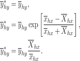
Jabeen et al.13 proposed the calibration estimators by taking motivation from Kim et al.8. The calibration estimator is given by
 |
where  is assumed to be a variable with a usual variance estimator exponential and ratio estimators, i.e.
 |
The calibration constraints, which define the relationship between the study variables and auxiliary variables, are defined by
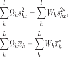 |
and
 |
Some proposed calibration variance estimators
In this section, we propose some new variance estimators to estimate the variation in the population using calibration technique.
Proposed calibration variance estimator
The following calibrated estimator is proposed to estimate the population variance, and it is defined by
 |
where
 |
with following constraints where  stratum.
 |
1 |
 |
2 |
and
 |
3 |
More details about the proof of the estimator  are given in “Appendix 1”.
Proposed calibration ratio estimator
We use the concept of Jabeen et al.13 and propose the initiated following calibration ratio estimator. The calibration ratio estimator is defined by
 |
where
 |
with the constraints mentioned in Eqs. (1) to (3),  stratum. The proof of proposed estimator
  is given in “Appendix 2”.
Proposed calibration exponential estimator
Following Jabeen et al.13, we propose the following calibration exponential estimator, which is defined as
 |
where
 |
with constraints given above in Eqs. (1), (2) and (3), where  stratum. Proof of the proposed estimator
  can be found in “Appendix 3”.
Simulation study
We produce distinctive simulated population where  and
and  values for various distributions, as given in Table 1. To obtain different levels of relationship among investigation and helping variable, we apply few transformations, which are given in Table 2.
Table 1.
Parameters and distribution of study (SV) and auxiliary variable (AV).
| No. | Parameters and distribution of SV | Parameters and distribution of AV |
|---|---|---|
| 1 |  |
 |
| 2 |  |
 |
| 3 |  |
 |
| 4 |  |
 |
Table 2.
Properties of each stratum.
| Strata | Study variable | Auxiliary variable |
|---|---|---|
| 1 Stratum |
 = 50 + = 50 + 
|
 = 15 + = 15 +  + + 
|
| 2 Stratum |
 = 150 + = 150 + 
|
 = 100 + = 100 +  + + 
|
| 3 Stratum |
 = 100 + = 100 + 
|
 = 300 + = 300 +  + + 
|
Each population comprises of three strata and each stratum contains 5 units. We choose  units from every stratum separately respectively, we get

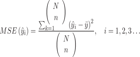
 = 2500 samples. The correlation coefficients between study variable and auxiliary variable for each stratum are taken as 0.5, 0.7 and 0.9 as per Tracy et al.17. The MSE is computed using following formula.
 |
The results of the MSE are presented in Tables 3, 4, 5 and 6. The results of simulated data presented in Table 3, 4, 5 and 6 are obtained for different distributions. In our analysis, we calculated the MSE for three proposed estimators across four different distributions with varying parameters, as detailed in Tables 1, 2, 3, 4, 5 and 6. The results, presented in Table 7, demonstrate that our proposed estimators consistently outperform the existing estimators by Isaki14 and Bahl and Tuteja15. Specifically, the MSE values for our estimators are consistently lower compared to those of the conventional estimators.
Table 3.
The MSE of the proposed estimators from gamma distribution.
| α,β | Estimator | MSE |
|---|---|---|
 |
 |
95,965.23 |
 |
177,237.1 | |
 |
79,867.68 | |
 |
 |
90,936.87 |
 |
177,145 | |
 |
74,138.4 | |
 |
 |
78,387.8 |
 |
141,730.5 | |
 |
44,512.85 |
Table 4.
The MSE of the proposed estimators from normal distribution.
| ρ | Estimator | MSE |
|---|---|---|
| 0.5 |  |
15,717.72 |
 |
4021.978 | |
 |
9922.135 | |
| 0.7 |  |
17,091.06 |
 |
2969.764 | |
 |
9631.747 | |
| 0.9 |  |
13,366.41 |
 |
2703.995 | |
 |
8005.757 |
Table 5.
The MSE of the proposed estimators from exponential distribution.
| λ | Estimator | MSE |
|---|---|---|
| 2 |  |
118,204.7 |
 |
238,458.8 | |
 |
151,247.1 | |
| 2.5 |  |
85,241.85 |
 |
171,522.5 | |
 |
57,668.86 | |
| 3.5 |  |
41,555.86 |
 |
82,738.78 | |
 |
6635.789 |
Table 6.
The MSE of the proposed estimators from log normal distribution.
| ρ | Estimator | MSE |
|---|---|---|
| 0.5 |  |
2,155,477 |
 |
3,011,671 | |
 |
2,237,658 | |
| 0.7 |  |
21,955,477 |
 |
1,291,763 | |
 |
2,120,258 | |
| 0.9 |  |
4,166,660 |
 |
2,458,213 | |
 |
1,920,386 |
Table 7.
Findings of the comparison of MSE across various estimators.
| MSE of t1 | MSE of t2 | MSE of t3 | MSE of Isaki14 | MSE of Bahl and Tuteja15 |
|---|---|---|---|---|
| 95,965.23 | 177,237.1 | 78,967.68 | 150,404.1 | 266,448 |
| 90,936.87 | 177,145 | 74,138.4 | 119,218 | 230,510.8 |
| 78,387.8 | 141,730.5 | 44,512.85 | 122,183.5 | 212,128.3 |
| 15,717.72 | 4021.978 | 9922.135 | 644,222 | 176,251.8 |
| 17,091.06 | 2969.764 | 9631.747 | 851,864.6 | 196,821.4 |
| 13,366.41 | 2703.995 | 8005.757 | 699,237.2 | 203,189.5 |
| 118,204.7 | 238,458.8 | 151,247.1 | 61,846,925 | 314,576.8 |
| 85,241.85 | 171,522.5 | 57,668.86 | 42,588,038 | 231,087.6 |
| 41,555.86 | 82,738.78 | 6635.789 | 21,837,626 | 132,359.2 |
| 2,155,477 | 3,011,671 | 2,237,658 | 4,686,898 | 6,131,997 |
| 2,195,253 | 1,291,763 | 2,120,258 | 2,401,915 | 6,684,994 |
| 4,166,660 | 2,458,213 | 1,920,386 | 6,806,558 | 6,790,442 |
These findings indicate that the proposed estimators provide more accurate and reliable results than their predecessors. Therefore, adopting our proposed estimators is likely to enhance performance and utility in practical applications.
Real life application
To demonstrate the performance of our proposed estimators, we use a real-life dataset from Koyuncu and Kadilar18. The dataset includes two variables: the number of teachers and the number of classes in both primary and secondary schools across Turkey. The data were collected from six diverse regions: Marmara, Aegean, Mediterranean, Central Anatolia, Black Sea, and East and Southeast Anatolia. A total sample size of  was selected, with the sample sizes for each stratum,
  , detailed in Table 8. The MSEs and their comparisons are presented in Table 9.
Table 8.
Summary statistics of six strata.
| N1 = 127 | N2 = 117 | N3 = 103 |
|---|---|---|
| N4 = 170 | N5 = 205 | N6 = 201 |
| n1 = 31 | n2 = 21 | n3 = 29 |
| n4 = 38 | n5 = 22 | n6 = 39 |
| Sy1 = 883.835 | Sy2 = 644.922 | Sy3 = 1033.467 |
| Sy4 = 810.585 | Sy5 = 403.654 | Sy6 = 711.723 |
 = 703.74 = 703.74 |
 = 413 = 413 |
 = 573.17 = 573.17 |
 = 424.66 = 424.66 |
 = 267.03 = 267.03 |
 = 393.84 = 393.84 |
| Cy1 = 1.256 | Cy2 = 1.562 | Cy3 = 1.803 |
| Cy4 = 1.909 | Cy5 = 1.512 | Cy6 = 1.807 |
| Sx1 = 30,486.751 | Sx2 = 15,180.769 | Sx3 = 27,549.697 |
| Sx4 = 18,218.931 | Sx5 = 8497.776 | Sx6 = 23,094.141 |
 = 20804.59 = 20804.59 |
 = 9211.79 = 9211.79 |
 = 14309.30 = 14309.30 |
 = 9478.85 = 9478.85 |
 = 5569.95 = 5569.95 |
 = 12997.59 = 12997.59 |
| CX1 = 1.465 | CX2 = 1.648 | CX3 = 1.925 |
| CX4 = 1.922 | CX5 = 1.526 | CX6 = 1.777 |
| Sxy1 = 25,237,153.52 | Sxy2 = 9,747,942.85 | Sxy3 = 28,294,397.04 |
| Sxy4 = 14,523,885.53 | Sxy5 = 3,393,591.75 | Sxy6 = 15,864,573.97 |
| ρ1 = 0.936 | ρ2 = 0.996 | ρ3 = 0.994 |
| ρ4 = 0.983 | ρ5 = 0.989 | ρ6 = 0.965 |
| w1 = 0.138 | w2 = 0.127 | w3 = 0.112 |
| w4 = 0.184 | w5 = 0.222 | w6 = 0.218 |
Table 9.
Comparison of the SEs of different estimators.
Table 9 displays the MSEs obtained from the proposed calibrated variance estimators—simple, ratio, and exponential—using the data provided in Table 8. The results align with those from the simulation studies. The comparison reveals that the proposed calibrated estimators are more efficient than existing estimators, as they exhibit the lowest MSEs. The application of the calibration technique enhances the overall performance of the estimators in estimating population variation.
Table 9 confirms that the results align with those obtained from the simulation studies. The comparison reveals that the proposed estimators using the calibration technique are more efficient than the existing ones, as they exhibit the lowest standard errors (SEs). This indicates that the calibration technique enhances the overall performance of the estimators in estimating population variation.
Conclusion
In this research, we introduced three new estimators inspired by Jabeen et al.13 to estimate population variation. We employed three calibration constraints and used the chi-square distance measure to minimize the discrepancy between the original and calibrated weights of strata. The three estimators developed are: the calibration variance estimator, the calibration ratio estimator, and the calibration exponential estimator. To assess the performance of these estimators, we analyzed the mean squared error (MSE) of both the proposed and existing estimators through simulation studies and real-life data. Our findings indicate that the proposed calibrated estimators outperform the existing ones, such as those by Isaki14 and Bahl and Tuteja15, by achieving a lower MSE.
Acknowledgements
The authors extend their appreciation to King Saud University for funding this work through Researchers Supporting Project number (RSPD2024R969), King Saud University, Riyadh, Saudi Arabia.
Appendix 1
Proof for the calibrated variance estimator
 |
The calibration constraints
 |
The following langrage’s function is given according to the distance measure and calibration constraints
 |
Differentiate w.r.t. 
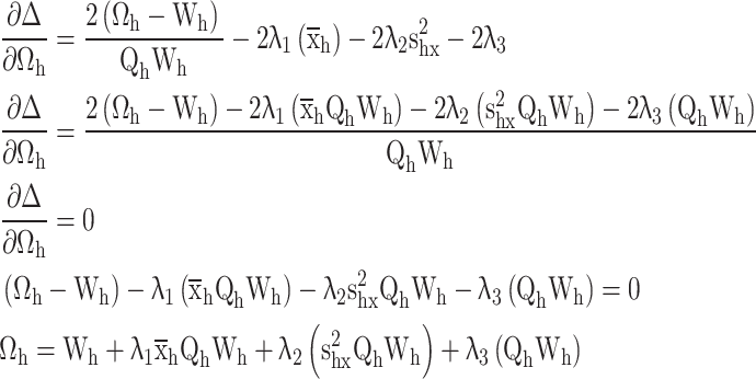 |
Substituting  in constraints
 |
 |
 |
 |
 |
 |
 |
 |
 |
 |
 |
Now put the  values in
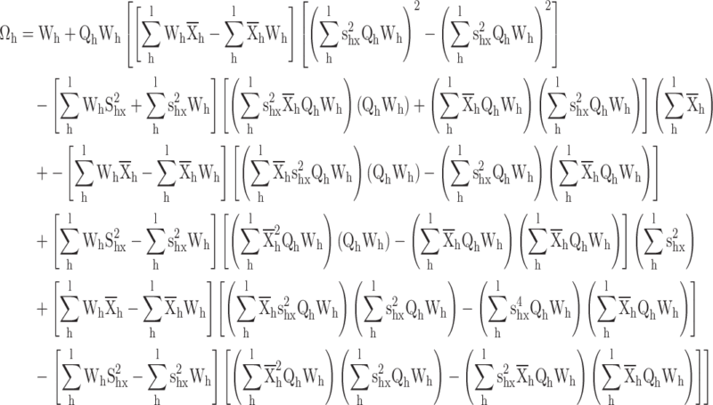 |
By putting the value of  , we get
The calibrated variance estimator
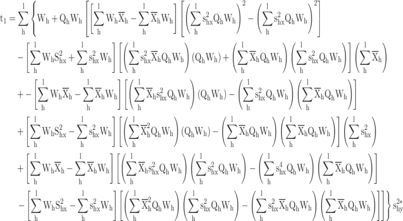 |
where  .
.
Appendix 2
Proof for the calibrated variance ratio estimator
 |
The calibration constraints
 |
The following langrage’s function is given according to the distance measure and calibration constraints
 |
Differentiate w.r.t. 
 |
Substituting  in constraints
 |
 |
 |
 |
 |
 |
 |
 |
 |
 |
 |
Now put the  values in
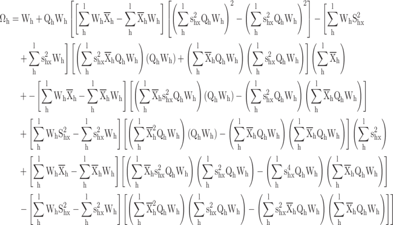 |
By putting the value of  , we get
The calibrated ratio variance estimator
 |
where  .
.
Appendix 3
Proof for the calibrated variance exponential estimator
 |
The calibration constraints
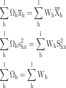 |
The following langrage’s function is given according to the distance measure and calibration constraints
 |
Differentiate w.r.t. 
 |
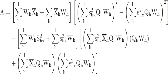
Substituting  in constraints
 |
 |
 |
 |
 |
 |
 |
 |
 |
 |
 |
Now put the  values in
 |
By putting the value of  , we get the calibrated exponential variance estimator is given by
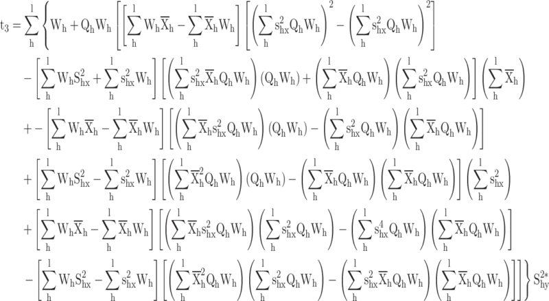 |
where  .
.
Author contributions
All authors reviewed the manuscript.
Funding
This research was conducted under a project titled “Researchers Supporting Project”, funded by King Saud University, Riyadh, Saudi Arabia under grant number (RSPD2024R969).
Data availability
The data used to support the findings of this study are included in the article.
Competing interests
The authors declare no competing interests.
Footnotes
Publisher’s note
Springer Nature remains neutral with regard to jurisdictional claims in published maps and institutional affiliations.
References
- 1.Graunt, J. The Economic Writings of Sir William Petty 1899 Vol. 2, 314–431 (Cambridge University Press, 1662). [Google Scholar]
- 2.Eren, H. Calibration process. In Handbook of Measuring System Design Vol. 3 (eds Sydenham, P. H. & Thorn, R.) 271–277 (Wiley, 2005). [Google Scholar]
- 3.Deville, J. C. & Särndal, C. E. Calibration estimators in survey sampling. J. Am. Stat. Assoc.87(418), 376–382 (1992). [Google Scholar]
- 4.Berge, A. Extension of calibration estimators in survey sampling. J. Am. Stat. Assoc.94, 635–644 (1999). [Google Scholar]
- 5.Estevao, V. M. & Särndal, C. E. A functional form approach to calibration. J. Off. Stat.16(4), 379 (2000). [Google Scholar]
- 6.Arnab, R. & Singh, S. A note on variance estimation for the generalized regression predictor. Aust. N. Z. J. Stat.47(2), 231–234 (2005). [Google Scholar]
- 7.Kott, P. S. Using calibration weighting to adjust for nonresponse and coverage errors. Surv. Methodol.32(2), 133–136 (2006). [Google Scholar]
- 8.Kim, J. M., Sungur, E. A. & Heo, T. Y. Calibration approach estimators in stratified sampling. Stat. Probab. Lett.77(1), 99–103 (2007). [Google Scholar]
- 9.Kim, J. K. & Park, M. Calibration estimation in survey sampling. Int. Stat. Rev.78(1), 21–29 (2010). [Google Scholar]
- 10.Koyuncu, N. & Kadilar, C. Calibration estimators using different measures in stratified random sampling. Int. J. Mod. Eng. Res.3(1), 415–419 (2013). [Google Scholar]
- 11.Bhushan, S., Kumar, A., Alsubie, A. & Lone, S. A. Variance estimation under an efficient class of estimators in simple random sampling. Ain Shams Eng. J.14, 102012 (2022). [Google Scholar]
- 12.Lone, S. A., Subzar, M. & Sharma, A. Enhanced estimators of population variance with the use of supplementary information in survey sampling. Math. Probl. Eng.2021, 1–8 (2021). [Google Scholar]
- 13.Jabeen, R., Aslam, M. & Zaka, A. Effects of different calibration constraints on calibration estimators under the randomized response technique. J. Stat. Comput. Simul.92(10), 1995–2017 (2022). [Google Scholar]
- 14.Isaki, C. T. Variance estimation using auxiliary information. J. Am. Stat. Assoc.78, 117–123 (1983). [Google Scholar]
- 15.Bahl, S. & Tuteja, R. K. Ratio and product type exponential estimators. J. Inf. Optim. Sci.12(1), 159–164 (1991). [Google Scholar]
- 16.Upadhyaya, L. N. & Singh, H. P. An estimator for population variance that utilizes the kurtosis of an auxiliary variable in sample surveys. Vikram Math. J.19, 14–17 (1999). [Google Scholar]
- 17.Tracy, D. S., Singh, S. & Arnab, R. Note on calibration in stratified and double sampling. Surv. Methodol.29(1), 99–104 (2003). [Google Scholar]
- 18.Koyuncu, N. & Kadilar, C. Ratio and product estimators in stratified random sampling. J. Stat. Plan. Inference139(8), 2552–2558 (2009). [Google Scholar]
Associated Data
This section collects any data citations, data availability statements, or supplementary materials included in this article.
Data Availability Statement
The data used to support the findings of this study are included in the article.


