Quasi-modified-Newton method-based selective harmonic elimination in cascaded H bridge inverters

Abstract

Multilevel converters have gained significant popularity in medium-voltage and high-power applications due to their numerous advantages over traditional two-level converters. These advantages include reduced harmonic distortion, improved efficiency, and lower stress on power semiconductors. Selective harmonic elimination (SHE) is a modulation method that can be employed with multilevel converters to achieve high-quality output voltage waveforms. In this work, an extension of Broyden’s method, known as the Quasi-Modified Newton Method, is implemented for selective harmonic elimination and accurate calculation of switching angles for a wide range of modulation indices. The proposed method is applied to cascaded H bridge inverters operating at levels 5, 7, and 9. The method offers simplicity, reduced computational burden, and faster convergence, making it easily implementable, reducing total harmonic distortion (THD), and reducing RMSE and MAD errors. The paper includes simulation and experimental results that validate the accuracy and effectiveness of the proposed approach.

Introduction

The Multilevel inverters are gaining popularity in various fields, including renewable energy systems, electric traction, industry, and smart grids, due to their capability to produce output voltages that closely resemble sinusoidal waveforms. When compared to traditional two-level converters, multilevel inverters produce a distinct waveform shape that offers significant advantages^1–3. These advantages include a decrease in total harmonic distortion (THD), enhanced efficiency, greater capacity to handle voltage and power, and reduced strain on components, resulting in improved dependability. The modulation technique used is the primary factor responsible for these characteristics, which has a significant impact on both performance and implementation complexity. Essentially, the modulation technique involves determining a set of switching angles, which serve as the unknowns in the modulation problem³.

Multilevel inverters have garnered considerable attention in medium-voltage and high-power applications, surpassing traditional two-level inverters^4–6. This is primarily due to their notable benefits, which include reduced switching losses, improved efficiency, lower common-mode voltage, and enhanced electromagnetic compatibility². The output waveform has more voltage steps when the number of voltage levels in a multilevel inverter goes up⁷. At the same time, the total harmonic distortion goes down.

There are algorithms for selective harmonic elimination (SHE), selective harmonic mitigation (SHM), and pulse width modulation (PWM) ⁸. Generally, SHE and SHM algorithms function at the fundamental frequency, whereas PWM algorithms operate at a higher frequency, albeit typically at lower values compared to conventional two-level PWM inverters. Lower frequencies typically yield higher overall efficiency, making them preferred^8,9. As a result, the adoption of SHE or SHM algorithms is desirable in scenarios where it is applicable, such as low-dynamic systems. On the other hand, applications that require high-bandwidth control commonly use multilevel PWM^10,11.

Recent work has focused on innovative algorithms for harmonic elimination in multilevel inverters, highlighting the effectiveness of approaches such as the Broyden’s Method Assisted Differential Evolution (BMADE) algorithm. This method effectively eliminates the third and fifth harmonics in the output voltage of a 7-level Cascaded H-Bridge Multilevel Inverter (CHB-MLI) through a selective harmonic elimination technique. This algorithm is not only applicable to hybrid cascaded multilevel inverter topologies but also extends to higher-level inverters and various optimization problems requiring enhanced accuracy²⁹. Additionally, the introduction of RDA optimization for a three-phase 11-level CHB-MLI fed by symmetric sources offers a promising solution for attenuating low-order harmonics while preserving the fundamental output voltage. This method proves effective in achieving optimal Total Harmonic Distortion (THD) values, further contributing to the enhancement of inverter performance³⁰.

Multilevel Pulse Width Modulation (PWM) inverters are becoming more important in many high-performance power applications, such as drives, active power filters, and static voltage compensators. One of their key advantages is that they do not need high ratings on individual devices. These inverters divide the DC rail, either directly or indirectly, enabling the output of each leg to encompass more than just two voltage levels¹². By combining amplitude modulation and pulse width modulation techniques, multilevel inverters enhance the quality of the output waveform, thereby reducing distortion. They offer a variety of benefits, including improved power quality, reduced switching losses, decreased output dv/dt, and increased voltage capacity. The power quality improves proportionally with the number of voltage levels in the inverter¹³. Two main pulse width modulation (PWM) schemes are utilized in multilevel inverters: Multicarrier sub-harmonic PWM (MC-SHPWM) and multicarrier switching frequency optimal pulse width modulation (MC-SFOPWM). When used in the diode-clamped multilevel inverter strategy, the MC-SHPWM technique effectively lowers the total harmonic distortion. Conversely, the MC-SFOPWM technique enhances the fundamental output voltage in the multilevel inverter strategy^14,15.

The Selective Harmonic Elimination (SHE) technique is utilized to reduce the Total Harmonic Distortion (THD) in an existing system. To achieve this goal, it is critical to identify and implement a method that can accurately determine the solutions for the equations involved in selective harmonic elimination (SHE) or a system of nonlinear equations that correspond to the converter’s switching angles. For this purpose, researchers have proposed several techniques such as iterative methods, optimization techniques, and mathematical solutions^16,17.

Broyden’s method

Broyden’s method (Fig. 1), introduced by C. G. Broyden, is a Quasi-Newton method used to determine roots in a system of equations with k variables. Finding approximate sets of solutions to a system of nonlinear equations is an improvement over Newton’s methods. Many researchers extended Newton’s method to the Quasi-Newton method or Broyden’s method to increase the convergence rate¹⁸. It is a generalization of the secant method. In comparison to Newton’s methods, its convergence rate is rapid, precise, and super-linear. Important characteristics include:

1. Reduced the number of scalar function evaluations from (n2 + n) to (n), but still requires O(n3) arithmetic operations.

2. Converge quickly with fewer errors.

Fig. 1.

Quasi-Newton Method Algorithm for a certain value of m.

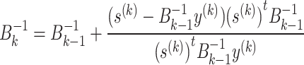
To solve the set of equations using this method, a set of initial guess values close to the exact solution is required, which leads to the actual solution. This method can only converge quickly if the initial value is sufficiently close to the exact solution. The absence of the need to calculate partial derivatives and inverses, which was one of Newton’s and Raphson’s flaws, is one of the other significant characteristics of this method. Calculating the Jacobian is unnecessary for this method. The method updates an approximation of another matrix at each iteration so that it behaves similarly to the actual Jacobian.

Initially, the matrix is set close to the true derivative of the set of values of the initial guess, considering it to be the actual Jacobian at iteration k. When the function f is ill-conditioned close to its root, Broyden’s method may experience difficulties. Ill-conditioning refers to a situation where minor alterations in the inputs can result in significant variations in the outputs, which can make it challenging to find an accurate root estimate. Additionally, while Broyden’s method can converge to a root of f, the sequence approximates Bk may not converge to the derivative of the function at the root. This is because Broyden’s method is a Quasi-Newton method that uses approximations of the derivative based on the differences in function values and input variables at different iterations. These approximations may not be accurate near the root, especially if the function is highly nonlinear or has singularities or other difficult features. Therefore, it is important to carefully monitor the convergence of Broyden’s method and to use other methods or techniques to verify the accuracy of the root estimate^19,20.

Despite its advantages of fast convergence, accuracy, and efficiency, one major problem stands out: how to initialize a value close enough to an exact solution to obtain convergence and a true value. Another problem is the number of arithmetic operations, which remains the same as in Newton’s methods: O(n3). To overcome these problems, we take into consideration an improved class of Broyden’s method and an extension of Broyden’s method.

Quasi modified Newton method

This Many engineering, mathematical, physical, and chemical problems result in nonlinear equations in applied mathematics, making scientists want to solve them to produce better and more accurate results. The Quasi-Modified Newton method (Fig. 2) was proposed by Yousef Abu Hour and Mohammad Al-Towaiq in 2017 as the extension class of Broyden’s or Quasi-Newton’s method for solving f(x). It is the fastest and most accurate iterative method. The procedure begins with an initial collection of close approximations to the precise solution. Through successive iterations, it gradually progresses towards a solution that fulfils the system of nonlinear equations. The method is an improvement of the Quasi-Newton method, which gives much more accurate and efficient results in comparison¹⁸.

Fig. 2.

Quasi-Modified Newton Method Algorithm for a certain value of m.

Some of the most significant features of this method include its simplicity. The main purpose of this method is to accelerate the rate of convergence of Quasi-Newton’s methods. The main benefits include:

Reduced number of function evaluations at each step from (n₂ + n) to just n and required O(n₂) arithmetic operations per iteration.

1. Reduced computational complexity

2. Improved accuracy

3. Evaluation of partial derivatives not required

4. Reduction in Root Mean Square Error (RMSE)

5. Total Harmonic Distortion Reduction

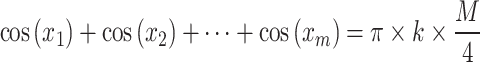
The objective of this approach is to apply the method to calculate precise switching angles for a system based on a set of given equations:

1

2

3

4

where x₁, x₂,…, x_m are the switching angles, n, n₁,…, n_q are the harmonic orders which need to be eliminated.

M is the modulation index, 2 k + 1 = Number of levels.

The switching angles are in the range 0 to π/2, where x₁ < x₂ < ⋯ < x_m < π/2.

The SHE can be implemented for p number of levels, which can be observed in the generalized equations:

5

6

7

It can be observed from the equations, number of switching angles increase, depending on the level on positive and the negative. For 5 level, there’s a 0 level and 2 positive and 2 negatives. It is such that because we need to control switching of each level to eliminate the harmonics. It can be the concluded that for every p level of inverter, number of switching angle required will be , for p levels we subtract the 0^th level and then divide by 2 to get the required number of switching angles, so the generalized equation would be as follows:

8

To apply the proposed method for higher order inverters, Eq. (8) needs to be solved using the algorithm, where n is harmonic order desired to eliminated, the total number of equations will thus depend on the harmonics which the user wants to eliminate. All the equations will be of the form of Eq. (8).

Different sets of solutions are obtained for different values of M. It can be noted that different sets of values for the initial guess may give different sets of solutions for the same value of M, but all the values of sets of solutions can be obtained (if they exist) if values of M vary in sufficiently small steps ¹⁹.

Steps to write the code:

1. Assume the given initial vector,

   9

2. Let B₀ = J

3. Compute

   10

   11

4. For k = 1

   Compute

   12

   13
5. Compute

   14
6. Compute

   15

   16

7. If , stop

Otherwise set k=k+1, continue looping

This will signify that the method has arrived at the system’s solution.

Selective harmonic elimination

Several suggestions have been made to improve the output quality of multilevel inverters. One method involves switching angles to eliminate lower harmonics, which is referred to as selective harmonic elimination (Fig. 3). To optimize the selection of switching angles, multilevel inverters (MLIs) primarily utilize selective harmonic elimination techniques. This method permits the generation of the desired fundamental output voltage while simultaneously eliminating lower harmonics. The idea behind selective harmonic elimination is to eliminate particular harmonics produced by a multilevel inverter by optimizing switching angles. In many instances, the optimization process tends to minimize overall harmonics, also known as total harmonic distortion, in addition to the specific targeted harmonics ^20,21.

Fig. 3.

Selective Harmonic Elimination implementation.

The SHE problem is formulated using Fourier series analysis as a set of nonlinear sets of trigonometric equations. More freedom is created as we take more angles into account. However, the main problem arises when solving the set of nonlinear equations. More switching angles increase the complexity of the equation. Many methods to solve the set of these equations have been proposed in the past. The three main methods include numerical iterative methods, evolutionary algorithms, and algebraic methods. Numerical iterative methods like Newton’s Raphson method have been used previously. To solve the problem using Newton Raphson, a good set of initial solutions must be chosen, close to the exact solution, which at some point appears to be a good problem. Evolutionary algorithms can give optimum switching angles for infeasible modulation indices ²².

For algebra-based methods, we do not need to use the initial set of solutions and can find the possible solutions. Staircase Selective Harmonic Elimination (SSHE) is a commonly used technique in Multilevel Inverters (MLIs) to achieve a wide output voltage range while simultaneously eliminating low-order harmonics.

Multilevel inverters (MLIs) are favored over conventional two-level inverters for several reasons. They have the capability to generate high-quality output voltage, minimize switching losses, reduce electromagnetic interference (EMI), and handle high levels of voltage and power. In an MLI, the output voltage is generated by connecting a series of capacitors and switches in a staircase-like configuration. By changing the switching states of the switches, the inverter can control the voltage levels at its output. However, the aforementioned characteristic also introduces harmonic distortion in the output waveform. To mitigate this issue, the Selective Harmonic Elimination (SSHE) technique is employed. This technique involves determining the optimal switching angles that yield the desired fundamental output voltage while simultaneously eliminating low-order harmonics. The SSHE technique achieves this by dividing the fundamental voltage waveform into multiple voltage steps and applying a staircase waveform to the inverter’s output. The staircase waveform is used to figure out the switching angles, and leaving out certain switching angles on purpose helps get rid of harmonic components in the output voltage ²³.

The SSHE technique proves to be highly advantageous in achieving a broad range of output voltages while ensuring a high level of voltage quality. By employing multiple voltage steps, it becomes feasible to attain a high resolution for the output voltage without introducing excessive levels of harmonic distortion. Moreover, the SSHE technique can be applied to different types of MLIs, including cascaded, neutral-point-clamped, and flying-capacitor MLIs. In this paper, we use a set of new iterative, super-linear, and fast methods in comparison to Newton methods for optimizing the switching angles and eliminating the multiple harmonics in multi-level inverters ²¹.

Selective harmonic elimination using quasi-modified Newton method

Using pulse modulation techniques for selective harmonic elimination is a way to reduce or get rid of certain harmonic components in the output waveform of a power electronic converter. Harmonics, which are unwanted frequency components, can lead to various problems in power systems, including increased losses, reduced efficiency, and interference with sensitive equipment. The pulse modulation technique involves controlling the switching instants of the power electronic switches in a converter to achieve the desired harmonic elimination ^8,24–28. The goal is to discover the most favourable switching angles or pulse patterns that lead to the cancellation or reduction of specific harmonics. To achieve the desired harmonic elimination, optimization algorithms, including numerical methods or iterative techniques, are utilized to determine the optimal switching angles. These algorithms aim to minimize the objective function by iteratively adjusting the switching angles until the desired level of harmonic elimination is achieved.

Here, we use the approach of the Quasi-Modified Newton Method to find the most optimal values of switching angles to achieve the minimum harmonic distortion possible. The main purpose of this method is to accelerate the rate of convergence. One of the major benefits of applying this method is its simplicity and efficient results, giving optimum results for switching angles. To apply SHE PWM, we perform Fourier analysis to obtain a set of nonlinear equations. The set of equations is solved by using Quasi-Modified Newton, which gives the values for switching angles. The values of the switching angle obtained are then used for applying the PWM technique for selective harmonic elimination, which results in a value of THD in per cent. The resultant value of THD comes out to be lower than the THD result using other numerical analysis methods, as discussed further in Section VII, thus proving its efficiency.

Here, the SHE problem is solved and implemented on a cascaded H bridge inverter. Figure 4 shows the general circuit of the cascaded H bridge inverter and the possible way of its extension to more levels.

Fig. 4.

Cascaded H-bridge inverter for k modules.

Results and comparative analysis

In this portion, the convergence characteristics, RMSE, and Median Absolute Deviation errors of Quasi-Modified Newton have been discussed and a comparison with the Newton–Raphson algorithm has been done.

Root Mean Square Error (RMSE) is a statistical metric that measures the average magnitude of errors between predicted and observed values in a dataset. It is commonly employed in various fields, including regression analysis, machine learning, and data science, to evaluate the performance of predictive models. The RMSE is calculated by taking the square root of the mean of the squared differences between predicted and observed values.

The formula for RMSE is as follows:

17

where n represents the number of data points in the dataset,

∑ indicates the sum of all the squared differences between predicted and observed values.

RMSE provides a single numerical value that represents the overall accuracy of a predictive model. RMSE is only one of several available evaluation metrics, and its interpretation must always be considered in the context of the specific problem domain and the nature of the analyzed data ²⁶.

Median Absolute Deviation (MAD) error provides a robust measure of central tendency because it is less sensitive to outliers compared to other metrics such as mean error. Outliers, which are extreme values that significantly deviate from the majority of the data, can distort the mean error. The median error, however, is less susceptible to outliers because it only considers the middle value ²⁶.

The MAD error formula is described as follows:

18

Figure 5 represents the MAD error in 5-level CHB using Quasi-Modified Newton and Newton Raphson. Comparing the values, the performance of Quasi-Modified Newton is better than Newton–Raphson, as it gives comparatively less error. RMSE and Median error are calculated for modulation index (m) = 0.9.

Fig. 5.

(a) MAD error for 5 levels using the Quasi-Modified Newton method. (b) MAD error for 5 levels using the Newton–Raphson algorithm.

Similarly, Fig. 6 represents the MAD error in 7-level CHB using Quasi-Modified Newton and Newton–Raphson.

Fig. 6.

(a) MAD error for 7 levels using the Quasi-Modified Newton method. (b) MAD error for 7 levels using the Newton–Raphson algorithm.

Comparing the values again, the performance of the Quasi-Modified Newton is better than that of Newton Raphson, as it gives comparatively less error.

Both RMSE and Median error are calculated for modulation index (m) = 0.9.

Similarly, the MAD error in 9-level CHB using the Quasi-Modified Newton and Newton Raphson is presented in Fig. 7. For modulation index (m) = 0.90, RMSE and Median error are both calculated.

Fig. 7.

(a) MAD error for 9 levels using the Quasi-Modified Newton method. (b) MAD error for 9 levels using the Newton–Raphson algorithm.

Comparing the values once more, the performance of Quasi-Modified Newton is superior to that of Newton–Raphson due to its relatively lower error rate.

Figure 8 illustrates the convergence graphs for different switching angles in a 5-level system. These graphs demonstrate that, despite being initialized with extreme values, all switching angles converge to a constant value. The convergence curves are shown using both the Quasi-Modified Newton method and Newton Raphson. Figure 9 illustrates the convergence graphs for various switching angles in a 7-level system, which are also initialized with extreme values and converge to the same constant value. Here, the convergence curves are also shown using both Quasi-Modified Newton method and Newton–Raphson. Figure 10 depicts convergence graphs for a 9-level system that, when initialized with extreme values, also converges to a constant value. Convergence curves using both algorithms are shown. Thus, the displayed convergence curves demonstrate that the Quasi-Modified Newton method converges rapidly and linearly when compared to Newton–Raphson.

Fig. 8.

(a) Convergence curves for 5^th levels when the initial value of θ₁ is set at 1º, 80º and 150^º using Quasi-Modified Newton method(b) Convergence curves for 5^th levels when the initial value of θ₂ is set at 1º, 80º and 150º using Quasi-Modified Newton method(c) Convergence curves for 5^th levels when the initial value of θ₁ is set at 1º, 80º and 150º using Newton—Raphson(d) Convergence curves for 5^th levels when the initial value of θ₂ is set at 1º, 80º and 150º using Newton Raphson.

Fig. 9.

(a) Convergence curves for 7^th levels when the initial value of θ₁ is set at 1º, 80º and 150° using the Quasi-Modified Newton method (b) Convergence curves for 7^th levels when the initial value of θ₂ is set at 1º, 80º and 150º using Quasi-Modified Newton method (c) Convergence curves for 7^th levels when the initial value of θ₃ is set at 1º, 80º and 150º using the Quasi Modified Newton method (d) Convergence curves for 7^th levels when the initial value of θ₁ is set at 1º, 80º and 150º using Newton Raphson (e) Convergence curves for 7^th levels when the initial value of θ₂ is set at 1º, 80º and 150º using Newton Raphson (f) Convergence curves for 7^th levels when the initial value of θ₃ is set at 1º, 80º and 150º using Newton Raphson.

Fig. 10.

(a) Convergence curves for the 9th level when the initial value of θ₁ is set at 1º, 80º and 150^º using Quasi-Modified Newton method (b) Convergence curves for the 9^th level when the initial value of θ₂ is set at 1º, 80º and 150º using Quasi-Modified Newton method (c) Convergence curves for the 9^th level when the initial value of θ₃ is set at 1º, 80º and 150º using Quasi-Modified Newton method (d) Convergence curves for the 9^th level when the initial value of θ₄ is set at 1º, 80º and 150º Quasi-Modified Newton method (e) Convergence curves for the 9^th level when the initial value of θ₁ is set at 1º, 80º and 150º Newton–Raphson (f) Convergence curves for the 9^th level when the initial value of θ₂ is set at 1º, 80º and 150º using Newton–Raphson (g) Convergence curves for the 9^th level when the initial value of θ₃ is set at 1º, 80º and 150º using Newton Raphson (h) Convergence curves for the 9^th level when the initial value of θ₄ is set at 1º, 80º and 150º using Newton Raphson.

Comparing the convergence graphs of Quasi-Modified Newton with Newton Raphson, the convergence rate of the Quasi-Modified Newton method is comparatively faster and linear.

Tables 1, 2, and 3 show the iteration number at which the switching angles start to converge using the Quasi-Modified Newton method and the Newton–Raphson algorithm, when the switching angles are set at 1°, 80°, and 150.

Table 1.

Switching angles Vs iteration number for 5 level.

Switching angles	Switching angles start to converge at iteration number
	Using Quasi Modified Newton (Number of Iterations required)			Using Newton Raphson (Number of Iterations required)
	Initial angle = 1°	Initial angle = 80°	Initial angle = 150°	Initial angle = 1°	Initial angle = 80°	Initial angle = 150°
θ1	50	50	82	65	60	90
θ2	45	35	85	55	40	90

Table 2.

Switching angles vs iteration number for 7 level.

Switching angles	Switching angles start to converge at iteration number
	Using Quasi Modified Newton (Number of Iterations required)			Using Newton Raphson (Number of Iterations required)
	Initial angle = 1°	Initial angle = 80°	Initial angle = 150°	Initial angle = 1°	Initial angle = 80°	Initial angle = 150°
θ1	25	50	78	40	62	86
θ2	83	75	62	82	80	79
θ3	35	48	47	35	68	61

Table 3.

Switching angles vs iteration number for 9 level.

Switching angles	Switching angles starts to converge at iteration number
	Using Quasi Modified Newton (Number of Iterations required)			Using Newton Raphson (Number of Iterations required)
	Initial angle = 1°	Initial angle = 80°	Initial angle = 150°	Initial angle = 1°	Initial angle = 80°	Initial angle = 150°
θ1	22	61	79	23	79	86
θ2	75	77	82	78	80	80
θ3	80	59	45	85	65	75
θ4	78	41	80	90	45	90

Figure 11 depicts box plots of RMSE versus the mean of switching angles. Figures 11(a) and 10(b) depict box plots of 5-level CHB inverters produced with the Quasi-Modified Newton method and Newton Raphson algorithm. Box plots of 7-level CHB inverters calculated using the Quasi Modified Newton Method and Newton Raphson algorithm are depicted in Fig. 11(c) and (d). Similarly, Fig. 11(e) and (f) depict the box plots of 9-level CHB inverters by using the Quasi Modified Newton method and Newton Raphson algorithm.

Fig. 11.

(a) Box plot of RMSE vs mean switching angles for a 5-level CHB inverter using the Quasi-Modified Newton method; (b) Box plot of RMSE vs mean switching angles for a 5-level CHB inverter using the Newton Raphson method (c) Box plot of RMSE vs mean switching angles for a 7-level CHB inverter using the Quasi-Modified Newton method; (d) Box plot of RMSE vs mean switching angles for a 7-level CHB inverter using the Newton Raphson method; (e) Box plot of RMSE vs mean switching angles for a 9-level CHB inverter using Quasi-Modified Newton method; (f) Box plot of RMSE vs mean switching angles for 9-level CHB inverter using Newton–Raphson algorithm.

The obtained results confirm, through a comprehensive comparative analysis, that the quasi-modified Newton Method outperforms the Newton–Raphson algorithm in terms of efficiency, speed, and super linear convergence. In Section 7, we compare the simulation outcomes of the Quasi-Modified Newton method and the Newton–Raphson Method.

Table 4 shows thee maximum, median and minimum values of RMSE using Quasi-Modified Newton method and Newton Raphson algorithm.

Table 4.

Maximum, median and minimum values for boxplot plotting RMSE using Quasi Modified Newton and Newton Raphson.

Levels of the inverter	Switching angles	Using Quasi Modified Newton			Using Newton Raphson
		Maximum value	Median value	Minimum value	Maximum value	Median value	Minimum value
5 level	θ1	0.80	0.48	0.34	1.10	0.69	0.51
	θ2	3.50	1.93	1.40	4.10	2.42	1.80
7 level	θ1	3.61	2.05	1.60	3.81	2.67	2.00
	θ2	12.80	9.28	7.13	13.66	10.77	8.12
	θ3	11.40	7.96	6.00	12.90	9.05	6.72
9 level	θ1	0.43	0.26	0.19	0.73	0.42	0.31
	θ2	1.40	0.77	0.59	1.60	1.05	0.78
	θ3	2.40	1.41	1.06	2.54	1.59	1.18
	θ4	2.23	1.37	1.01	2.30	1.61	1.19

Table 5 highlights the differences between the two algorithms. The parameters include convergence rate, ease of computation and complexity of the algorithms Quasi Modified Newton and Newton–Raphson. The plots depict the errors observed when employing both the Quasi-modified Newton and Newton–Raphson algorithms. The results show that the Quasi-Modified Newton method has significantly fewer errors than the Newton–Raphson algorithm, demonstrating its superior performance.

Table 5.

Comparison of the algorithms.

Parameters	Quasi-Modified Newton	Newton–Raphson
Convergence	The algorithm converges faster, it takes a smaller number of iterations, which can be observed in Figs. 7, 8 and 9	The algorithm, in comparison, takes a greater number of iterations to converge, which can be observed in Figs. 7,8 and 9
Computation	Computation is easier comparatively. Here, while evaluating, partial derivative and Jacobian matrix need not be calculated in every step. The algorithm initializes the Jacobian matrix with the variables	Computation is comparatively not easier while evaluating the algorithm requires calculating the partial derivative and Jacobian matrix in every step
Complexity	The algorithm’s complexity is reduced, as the number of function evaluations in each step from n2 + n to n. It also requires O(n2) operation per iteration	In this algorithm, the number of evaluations in each step is n2 + n. It requires O(n3) operations per iteration

Table 6 shows the results taken using Quasi Modified Newton and Newton Raphson tabulated for ease.

Table 6.

Results tabulated.

Results	Using Quasi Modified Newton	Using Newton Raphson
Voltage THD % for 5 level	17.96	18.77
Voltage THD % for 7 level	10.90	13.26
Voltage THD % for 9 level	10.05	10.20
RMSE Error	With reference to Table 4 and Fig. 11, RMSE error is reduced	With reference to Table 4 and Fig. 11, RMSE error is comparatively high
MAD Error	With reference to Figs. 5,6 and 7, MAD error is reduced	With reference to Figs. 5, 6 and 7, MAD error is comparatively high
Convergence	With reference to Tables 1,2 and 3 and Figs. 8, 9 and 10, convergence is fast	With reference to Tables 1,2 and 3 and Figs. 8, 9 and 10, convergence is comparatively slow

Simulation results and discussion

MATLAB platform has been utilized to execute the Quasi-Modified Newton method, which returns all possible combinations of switching angles for varying modulation index m. Figures 12, 13, and 14 show the switching angles for modulation indices from 0.5 to 1 when applied to 5, 7, and 9-level cascaded H bridge (CHB) inverters. These angles are based on a certain set of initial solutions.

Fig. 12.

Switching angles for a 5-level CHB converter.

Fig. 13.

Switching angles for a 7-level CHB converter.

Fig. 14.

Switching angles for 9-level CHB converter.

Total Harmonic Distortion (THD) is a measurable method for determining the level of signal distortion. As the harmonic amplitudes increase, so do the distortions.

The optimal switching angle values result in the lowest THD. For all three 5, 7, and 9 CHB topologies, 8 switches have been used and simulated on MATLAB Simulink. A single-cascaded H bridge 5-level inverter is used to drive the RL load (R = 50Ω and L = 8 mH) with DC sources for each H bridge inverter circuit as V_d1 = V_d2 = 100 V. Using MATLAB/Simulink, FFT analysis and the simulation output voltage and current waveform are shown in Figs. 15 and 16 respectively. The switching angles for 5-level CHB for eliminating the 5th harmonic are θ₁ = 16.32° and θ₂ = 52.36°, with modulation index = 0.9, giving the THD as 17.9%. The 5th harmonic is eliminated as it is presented only by 0.67%, which is less than 1%. Some other higher harmonics in the percentages) that are present have been shown in Table 7.

Fig. 15.

5^th harmonic elimination.

Fig. 16.

Output voltage and current waveform.

Table 7.

Percentage of other harmonics present.

Harmonic Order	Percentage (%)
3rd	2.67
7th	7.02
9th	4.08
11th	10.83
13th	3.38
15th	0.56
17th	3.68
19th	2.13

For a seven-level CHB inverter, the parameters for RL load are R = 100 ohms and L = 5 mH, with DC sources for H bridge 1 as V_d1 = 100 V and V_d2 = 2V_d1 = 200 V. The switching angles for 7-level inverters for eliminating the 5th and 7th harmonics are θ₁ = 14.8°, θ₂ = 39.07°, and θ₃ = 62.7°. The modulation index is 0.9, giving a THD of 10.90%. The 5th and 7th harmonics are present at 0.05% and 0.8%, respectively. Some other higher harmonics (in the percentages) that are present have been shown in Table 8. Figures 17 and Fig. 18 present the harmonic profile along with the output voltage and current waveform respectively.

Table 8.

Percentage of other harmonics present.

Harmonic order	Percentage (%)
3rd	1.35
9th	4.33
11th	1.21
13th	5.54
15th	0
17th	6.54
19th	4.13

Fig. 17.

5^th and 7^th harmonic eliminations.

Fig. 18.

Output voltage and current waveform.

The parameters for driving the RL load for the nine-level CHB inverter are R = 50 Ω and L = 8 mH with DC sources for H bridges as V_d1 = 30 V and V_d2 = 3V_d1 = 90 V. The switching angles for eliminating the 5th, 7th, and 11th harmonics are θ₁ = 10.23°, θ₂ = 23.43°, θ₃ = 43.42° and θ₄ = 63.22° with modulation index = 0.9 for a random initial set of values, giving the THD as 10.05%. The fifth, seventh, and eleventh harmonics are responsible for 0.37 percent, 0.15 percent, and 1.17 percent, respectively. Some other higher harmonics (in the percentages) that are present have been shown in Table 9. The Harmonic profile along with the output voltage and current waveform are shown in Figs. 19 and Fig. 20 respectively.

Table 9.

Percentage of other harmonics present.

Harmonic order	Percentage (%)
3rd	3.49
9th	2.34
13th	2.73
15th 17th	1.33 3.67
19th	1.67

Fig. 19.

5^th, 7^th and 11^th harmonic elimination.

Fig. 20.

Output voltage and current waveform.

Figure 21 shows the voltage and current waveforms for 5, 7 and 9 levels when modulation index is changed from 0.5 to 0.9. These graphs show the performance of the algorithm at extreme modulation indices.

Fig. 21.

(a) 5-level voltage and current waveforms at 0.5 modulation index and changing to modulation index 0.9 (b) 7-level voltage and current at 0.5 modulation index and changing to modulation index0.9 (c) 9-level voltage and current at 0.5 modulation index and changing to modulation index 0.9.

Using the Newton–Raphson method with the same modulation index and eliminating the 5th harmonic, we get a THD of 18.77%, as shown in Fig. 22. For a 7-level CHB inverter, using the N-R algorithm for eliminating 5th and 3rd, the THD is given as 13.06%. Figure 23 depicts the elimination of the fifth and seventh harmonics using the N-R algorithm, along with a THD of 10.20%. Figure 24 depicts the elimination of the fifth, seventh, and eleventh harmonics using the N-R algorithm, along with a THD of 10.20%.

Fig. 22.

Elimination of 5^th harmonic using Newton Raphson algorithm.

Fig. 23.

Elimination of 5^th and 7^th harmonics using Newton Raphson algorithm.

Fig. 24.

Elimination of the 5th, 7th, and 11th harmonics using the Newton–Raphson algorithm.

The preceding analysis demonstrates that the Quasi-Modified Newton improves THD clearly and significantly, demonstrating its efficacy and efficiency. This is a table. Tables should be placed in the main text near to the first time they are cited.

Hardware results

This portion demonstrates the practical application of the Quasi-modified Newton Method on a cascaded H-bridge inverter. Figure 25 shows the experimental setup in the laboratory for the verification of the Quasi-Modified Newton method on a CHB 8-switch inverter.

Fig. 25.

Experimental set-up in the lab.

On the Digital Storage Oscilloscope (DSO), it is possible to observe the output waveforms. Figure 25 depicts the voltage and current waveforms of the load for 5-level, 7-level, and 9-level inverters, respectively. The outcomes for both resistive and resistive-inductive loads are provided. Following the application of the Quasi-Modified Newton method, these results depict the current and voltage waveforms in CHB inverters with and without harmonics. Figure 26. (a), (b) shows experimental results of 5-level CHB inverters supplied with R load impedance Z = 40 Ω and R-L load impedance Z = 40 Ω for modulation index (m) = 0.69. Figure 26. (c), (d) shows experimental results for 7-level CHB inverters supplied with R-load impedance Z = 25 Ω and R-L load impedance Z = 25 Ω ohms for modulation index (m) = 0.72. Figure 26. (e), (f) shows experimental results for 9-level CHB inverters supplied with R load impedance, Z = 20Ω and for R-L load impedance, Z = 10Ω for modulation index (m) = 0.79. Figure 26 (g), (h) and (i) shows the experimental results for 5-level, 7-level and 9-level voltage and current waveforms on varying loads. Here, the load is simultaneously varied.

Fig. 26.

(a) Hardware results showing voltage and current waveforms and harmonics present for a 5-level CHB inverter on R-load. (b) Hardware results showing voltage and current waveforms and harmonics present for a 5-level CHB inverter on RL-load. (c) Hardware results showing voltage and current waveforms and harmonics present for a 7-level CHB inverter on R-load. (d) Hardware results showing voltage and current waveforms and harmonics present for 7-level CHB inverter on R-load. (e) Hardware results showing voltage and current waveforms and harmonics in a 9-level CHB inverter on R-load. (f) Hardware results showing voltage and current waveforms and harmonics in 9-level CHB inverters on an R-L load. (g) 5-level voltage and current waveforms on varying loads. (h) 7-level voltage and current waveforms on varying loads (i) 9-level voltage and current waveforms on varying loads.

These experimental results validate the simulation results, verifying the efficiency of the Quasi-Modified Newton method.

Conclusion

This paper utilizes the Quasi-Modified Newton Method to compare the total harmonic distortion (THD) results for three multilevel inverters: 5-level, 7-level, and 9-level. The important conclusion includes:

1. Reduced computational complexity

2. Improved accuracy

3. Evaluation of partial derivatives not required

4. Reduction in Root Mean Square Error (RMSE)

5. Total Harmonic Distortion Reduction

For a highly nonlinear, multivariable problem and higher-order harmonics, the proposed algorithm fails to converge and does not provide the optimal switching angle.

Application of the proposed methodology for solving the SHE problem lies in optimizing the switching angles, which in turn eliminate the harmonics more effectively and reducing the THD %, thus improvising the efficiency of the inverter.

The findings of this paper demonstrate that the Quasi-Modified Newton Method outperforms the Newton–Raphson method. When all other factors remain constant, the simulation results show that the new method achieves a lower THD than the Newton–Raphson method. Furthermore, the Quasi-Modified-Newton Method offers more accurate and faster results compared to the Newton–Raphson method. Also, a hardware implementation was done to confirm the simulation results for both resistive (R) and resistive-inductive (R-L) loads at certain modulation indices.

Author contributions

Conceptualization, B. S., U. M., A. S., and S. A..; formal analysis, B. S., and U. M.; inves-tigation, B. S., and U. M.; software, B. S., and U. M.; methodology, B. S., and U. M.; data curation, B. S., U. M., and A. S..; visualization: B. S., and U. M.; funding acquisition, H.-D. L.; supervision, H.-D. L.; writing—original draft, B. S., U. M., A. S., S. A., L.-Y. H., and H.-D. L.; writing—review and editing, B. S., U. M., A. S., S. A., L.-Y. H., and H.-D. L.

Funding

This research has received funding from King Saud University through Researchers Supporting Project number RSP2024R387), King Saud University, Riyadh, Saudi Arabia.

Data availability

The datasets used and/or analysed during the current study available from the corresponding author on reasonable request.

Declarations

Competing interests

The authors declare no competing interests.

References

- 1.Sarwer, Z., Anwar, M. N. & Sarwar, A. A nine-level common ground multilevel inverter (9L-CGMLI) with reduced components and boosting ability. Int. J. Circuit Theory Appl.10.1002/cta.3550 (2023). [Google Scholar]
- 2.Khan, R. A. et al. Archimedes optimization algorithm based selective harmonic elimination in a cascaded h-bridge multilevel inverter. Sustainability (Switzerland), 14(1). 10.3390/su14010310 (2022).
- 3.Bhoopal, N., Rao, D. S. M., Narukullapati, B. K., Kasireddy, I. & Kumar, D. G. Selective Harmonic Elimination Based THD Minimization of a Symmetric 9-Level Inverter Using Ant Colony Optimization. Math. Model. Eng. Probl.8(5), 769–774. 10.18280/mmep.080512 (2021). [Google Scholar]
- 4.Chabni, F., Taleb, R. & Helaimi, M. ANN-based SHEPWM using a harmony search on a new multilevel inverter topology. Turk. J. Electr. Eng. Comput. Sci.25(6), 4867–4879. 10.3906/elk-1703-122 (2017). [Google Scholar]
- 5.Gao, L., Liu, Y., Chen, N., Li, H., Zhang, N., & Yu, S. A Design method of the transmitting waveform of electromagnetic sounding based on selective harmonic elimination. Math Probl Eng, 2022. 10.1155/2022/2915275 (2022).
- 6.Kumari, M., Sarwar, A., Tariq, M., Ahmad, S., Mohamed, A. S. N., & Rodrigues, E. M. G. A symbiotic organism search-based selective harmonic elimination in a switched capacitor multilevel inverter. Energies (Basel). 15(1). 10.3390/en15010089 (2022).
- 7.Yaqoob, M. T., Rahmat, M. K., Maharum, S. M. M. & Su’ud, M. M. A review on harmonics elimination in real time for cascaded h-bridge multilevel inverter using particle swarm optimization. Int. J. Power Electron. Drive Syst.12(1), 228–240. 10.11591/ijpeds.v12.i1.pp228-240 (2021). [Google Scholar]
- 8.Xie, D. et al. Diagnosis and Resilient Control for Multiple Sensor Faults in Cascaded H-Bridge Multilevel Converters. IEEE Trans Power Electron, pp. 1–15, 10.1109/TPEL.2023.3279907 (2023).
- 9.Poorfakhraei, A., Narimani, M. & Emadi, A. A review of modulation and control techniques for multilevel inverters in traction applications. IEEE Access9, 24187–24204. 10.1109/ACCESS.2021.3056612 (2021). [Google Scholar]
- 10.Prabaharan, N. & Palanisamy, K. A comprehensive review on reduced switch multilevel inverter topologies, modulation techniques and applications. Renew Sustain Energy Rev76, 1248–1282. 10.1016/j.rser.2017.03.121 (2017). [Google Scholar]
- 11.Urmila, B. & Subbarayudu, D. Multilevel inverters: a comparative study of pulse width modulation techniques. Int. J. Sci. Eng. Res. 1(3), [Online]. Available: http://www.ijser.org (2010).
- 12.Tayyab, M. et al. Grid-connected operation and control of single-phase asymmetrical multilevel inverter for distributed power generation. IET Renew. Power Gener.16(16), 3629–3642. 10.1049/rpg2.12581 (2022). [Google Scholar]
- 13.Urgun, S. & Yigit, H. Selective harmonic eliminated pulse width modulation (SHE-PWM) method using genetic algorithm in single-phase multilevel inverters. Int. J. Electr. Eng. Inform.13(1), 191–202. 10.15676/IJEEI.2021.13.1.11 (2021). [Google Scholar]
- 14.Adeyemo, I. A., Ojo, J., Adegbola, O., Adeyemo, I. A., & Adegbola, J. A. Selective harmonic elimination in standalone single-phase multilevel inverter connected to photovoltaic array smart energy management system for homes view project unpaved-road extraction from satellite images (Master’s Thesis) view project selective harmonic elimination in standalone single-phase multilevel inverter connected to photovoltaic array. 10.22624/AIMS/DIGITAL/V10N3P9xx (2022).
- 15.Khizer, M. et al. Selective harmonic elimination in a multilevel inverter using multi-criteria search enhanced firefly algorithm. IEEE Access11, 3706–3716. 10.1109/ACCESS.2023.3234918 (2023). [Google Scholar]
- 16.Moussa, M. F., & Dessouky, Y. G. Selective harmonic elimination in multi-level inverter with selective harmonic elimination in multi-level inverter with equal-power-rating series-connected transformers. 10.6113/JPE.2014.14.1.
- 17.Yi H’ng, C., Ismail, B., Khairul, M. N., & Rohani, H. Selective Harmonic Elimination Pulse Width Modulation for Five-Level Cascaded Inverter.
- 18.Hour, Y. A. & Al-Towaiq, M. Extension Classes of Broyden’s and Central Broyden’s Methods for Solving F (x) = 0. [Online]. Available: https://www.researchgate.net/publication/323186145 (2017).
- 19.Broyden, C. G. A Class of methods for solving nonlinear simultaneous equations.
- 20.Toubal, A. E. et al. Mathematical analysis of N-R algorithm for experimental implementation of SHEPWM control on single-phase inverter. Int. J. Eng. Trends Technol. (IJETT), [Online]. Available: http://www.ijettjournal.org
- 21.Yaqoob, M. T., Rahmat, M. K., & Maharum, S. M. M. Modified teaching learning based optimization for selective harmonic elimination in multilevel inverters. Ain Shams Eng. J.13(5). 10.1016/j.asej.2022.101714 (2022).
- 22.Vivert, M., Diez, R., Cousineau, M. Bernal Cobaleda, D., Patino, D., & Ladoux, P. Real-time adaptive selective harmonic elimination for cascaded full-bridge multilevel inverter. Energies (Basel)15(9). 10.3390/en15092995 (2022).
- 23.Parihar, M., Singh, G., Bhaskar, M. K., & Jain, D. Analysis of cascaded H-bridge multilevel solar inverter. Int. J. Eng. Tech. 8. 10.5281/zenodo.7221140. (2022)
- 24.Laali, S. & Nasiri-Zarandi, R. New cascaded multilevel inverter with series connection of novel capacitor based basic units. IET Power Electron.10.1049/pel2.12502 (2023). [Google Scholar]
- 25.Sajid, I., Sajid, J., Azad, M. A., & Sarwar, A. A Novel Seven-Level Switched Capacitor Multilevel Inverter Topology with Common Ground Configuration. In: 2023 International Conference on Power, Instrumentation, Energy and Control, PIECON 2023, Institute of Electrical and Electronics Engineers Inc. 10.1109/PIECON56912.2023.10085748. (2023).
- 26.Hodson, T. O. Root-mean-square error (RMSE) or mean absolute error (MAE): when to use them or not. Geosci. Model Dev.15(14), 5481–5487. 10.5194/gmd-15-5481-2022 (2022). [Google Scholar]
- 27.Ali, M., Tayyab, M., Sarwar, A. & Khalid, M. A low switch count 13-level switched-capacitor inverter with Hexad voltage-boosting for renewable energy integration. IEEE Access10.1109/ACCESS.2023.3265467 (2023). [Google Scholar]
- 28.Alnuman, H. et al. A single-source switched-capacitor 13-level high gain Inverter with lower switch stress. IEEE Access10.1109/ACCESS.2023.3266050 (2023). [Google Scholar]
- 29.Ahsan, M. et al. Broyden’s method assisted differential evolution (BMADE) based selective harmonic elimination in a cascaded H-bridge multilevel inverter. IET Power Electron.16, 2336–2355. 10.1049/pel2.12553 (2023). [Google Scholar]
- 30.Bulletin of Electrical Engineering and Informatics 12(5), 2643–2650. 10.11591/eei.v12i5.5160. ISSN: 2302-9285 (2023)
Associated Data
This section collects any data citations, data availability statements, or supplementary materials included in this article.
Data Availability Statement