

Abstract
Background:
The prevalence of toxic chemicals in US commerce has prompted some states to adopt laws to reduce exposure. One with broad reach is California’s Proposition 65 (Prop 65), which established a list of chemicals that cause cancer, developmental harm, or reproductive toxicity. The law is intended to discourage businesses from using these chemicals and to minimize consumer exposure. However, a key question remains unanswered: Has Prop 65 reduced population-level exposure to the listed chemicals?
Objective:
We used national biomonitoring data from the Centers for Disease Control and Prevention (CDC) to evaluate the impact of Prop 65 on population-level exposures.
Methods:
We evaluated changes in blood and urine concentrations of 37 chemicals (including phthalates, phenols, VOCs, metals, PAHs, and PFAS), among US National Health and Nutrition Examination Survey (NHANES) participants in relation to the time of chemicals’ Prop 65 listing. Of these, 11 were listed prior to, 11 during, and 4 after the biomonitoring period. The remaining 11 were not listed but were closely related to a Prop 65-listed chemical. Where biomonitoring data were available from before and after the date of Prop 65 listing, we estimated the change in concentrations over time for Californians compared with non-Californians, using a difference-in-differences model. We used quantile regression to estimate changes in exposure over time, as well as differences between Californians and non-Californians at the 25th, 75th, and 95th percentiles.
Results:
We found that concentrations of biomonitored chemicals generally declined nationwide over time irrespective of their inclusion on the Prop 65 list. Median bisphenol A (BPA) concentrations decreased 15% after BPA’s listing on Prop 65, whereas concentrations of the nonlisted but closely related bisphenol S (BPS) increased 20% over this same period, suggesting chemical substitution. Californians generally had lower levels of biomonitored chemicals than the rest of the US population.
Discussion:
Our findings suggest that increased scientific and regulatory attention, as well as public awareness of the harms of Prop 65-listed chemicals, prompted changes in product formulations that reduced exposure to those chemicals nationwide. Trends in bisphenols and several phthalates suggest that manufacturers replaced some listed chemicals with closely related but unlisted chemicals, increasing exposure to the substitutes. Our findings have implications for the design of policies to reduce toxic exposures, biomonitoring programs to inform policy interventions, and future research into the regulatory and market forces that affect chemical exposure. https://doi.org/10.1289/EHP13956
Introduction
Human exposure to the chemicals in active commerce in the United States, many of which are known or suspected to be toxic, is a source of increasing concern.1 To address gaps and weaknesses in federal chemicals law, states have adopted a range of bans, restrictions, and right-to-know laws applicable to toxic chemicals.
California’s Proposition 65 right-to-know law (Prop 65)2 was intended to use the power of information to discourage businesses from using toxic chemicals, as well as to help consumers limit their personal exposure to toxics. Prop 65 was passed by ballot initiative in 1986 in response to widespread concern about underregulation of toxic chemicals. The law requires the State of California to identify chemicals that cause cancer, birth defects, or reproductive harm.3,4 Chemicals are added to the Prop 65 list either automatically when they are designated by another authoritative body as a carcinogen or a reproductive or developmental toxicant, or after independent, in-depth scientific review by committees designated as the State’s Qualified Experts, which meet at least once annually.5 The Prop 65 list now includes listings, of which are unique chemicals.
Businesses are required to warn the public when their products, processes, premises, or releases to the environment are likely to cause exposures to listed chemicals above a certain risk threshold.6 The duty to warn the public of potentially harmful exposures to Prop 65-listed chemicals has engendered cautionary statements accompanying a wide range of consumer products and processed foods, in residential and commercial buildings, in workplaces, and at industrial facilities throughout the state.7 Businesses’ impulse to avoid the legal duty to warn has also prompted some to eliminate or reduce listed chemicals in many consumer products and to lower air emissions and effluent discharge of Prop 65 chemicals.8–11
The varied effects of Prop 65 have spawned significant scholarship and popular press focused on the warning fatigue that abundant Prop 65 warnings may generate for consumers,6,12 and more positively, the indirect effects of Prop 65 in advancing chemical regulation and providing information about toxic chemical exposures in both the manufacturing sector and the public sphere more generally.7 Despite the attention that Prop 65 has received and its potential impact on commerce and consumer behavior, researchers have been unable to answer a key question: Are Prop 65 chemical listings associated with changes in population-level exposures to toxic chemicals within California, or even nationwide?
Systematic evaluation of the effect of environmental policies on chemical exposures over time at a population level requires data that represents the population of interest, includes a comparison group, and has been collected longitudinally using consistent methods over time.13,14 In the United States, the only chemical biomonitoring conducted for surveillance of general population health is within the laboratory component of the National Health and Nutrition Examination Survey (NHANES) conducted by the Centers for Disease Control and Prevention (CDC).15 The NHANES biomonitoring program has been continuously administered since 1999, with results published biannually. Analytical methods and measured chemicals are relatively consistent over time, enabling time trend analyses, although chemicals are regularly added and dropped and analytical methods are modified.16 Chemicals that the CDC selects for nationwide biomonitoring are generally those that have already prompted public health concern.17 Our analysis encompassed biomonitoring data for chemicals listed on Prop 65 both before and during the biomonitoring period (1999–2016).
NHANES is not expressly intended for geographic comparisons. NHANES is designed to be nationally representative, and participants are selected from 15 locations across the United States each year.18 The data can nonetheless reveal spatial variability that may suggest drivers of differential exposure, some of which track geographically. For example, NHANES data show that women of reproductive age living in coastal areas have higher blood mercury levels than women living inland, a phenomenon attributed to different patterns of fish consumption.19 Other exposure differentials track local differences in chemical regulations: NHANES measurements of urinary cotinine, a metabolite of nicotine, show that nonsmokers living in counties that restrict smoking in public spaces are exposed to significantly less cigarette smoke than are nonsmokers living in counties without smoking restrictions.20
Evaluating the effects of Prop 65 chemical listings is significantly more challenging than evaluating the effects of a single-chemical policy given the enormous number of chemicals Prop 65 encompasses, as well as the diverse mechanisms by which it might affect exposure to toxics. These complexities notwithstanding, we used publicly available NHANES biomonitoring data, supplemented by data on California vs. non-California state of residence obtained from the National Center for Health Statistics (NCHS) Research Data Center (RDC), to probe associations between the timing of chemicals’ listing on Prop 65 and changes in US residents’ exposures. Prop 65 chemical listing requires businesses to warn relevant parties—such as consumers and workers —of their potential for chemical exposure and threatens legal liability for noncompliance. Prop 65 listings are therefore expected (and have been shown) to affect business and consumer behavior in ways that could reduce exposure.8,9 Further, it is well established that where manufacturers reformulate in response to a Prop 65 listing, they typically do so on a nationwide basis.7
In this analysis, first, we examined whether levels of listed chemicals decreased in national biomonitoring data after listing. Second, we examined whether there were differences in trends between biomonitored concentrations in Californians and the rest of the US population, which might reflect influences of Prop 65 in California. For example, where manufacturers opt to warn consumers about Prop 65 chemicals in a product rather than to reformulate, warnings are only required for products sold in California. Further, Prop 65 listings and enforcement actions are covered in the California press more than in national press, which might prompt Californians to take actions to reduce personal exposure. Third, we looked at chemicals that had not been listed under Prop 65 but were structurally related to listed chemicals, to discern the extent to which Prop 65 prompts market substitutions. We further examined whether exposure trends at the upper end of the concentration distribution (75th and 95th percentiles) differed from trends in mean concentrations, on the theory that lowering exposures for people with the highest concentrations could have particular public health significance.
Methods
NHANES Data and Analyte Selection
We downloaded the Prop 65 list (as of December 2021) from the California Office of Environmental Health Hazard Assessment (OEHHA).21 The list includes the chemical name, Chemical Abstract Service (CAS) number, date of listing, and a chemical’s classification as a carcinogen, reproductive toxicant, developmental toxicant, or listing for more than one of these endpoints. Typically, several chemicals are listed each year. Chemicals are rarely removed from the list.
We analyzed laboratory, demographic, and restricted (not publicly available) NHANES data from the period 1999–2016. Each year, the NHANES program visits 15 study locations, typically defined as counties (adjacent counties are sometimes combined to maintain a minimum size). NHANES employs a four-stage sampling design to ensure a nationally representative sample of the US population, with people included each year. In the first and second stages, primary sampling units (usually counties) in stage 1, and segments (such as city blocks) in stage 2, are selected with probability proportional to their size. In stages 3 and 4 (households and individuals), sampling is random within the selected segments. To ensure greater stability of statistical estimates, data are publicly released in 2-y cycles.18 NHANES screens participant samples for environmental chemical analytes that are grouped into panels of structurally similar chemicals and measured together, with most panels measured in subsamples of one-third of the participants. NHANES study protocols are reviewed and approved by the NCHS Research Ethics Review Board, and participants provide informed consent.16
We chose analytes of chemicals on the Prop 65 list, with particular attention to those listed during the biomonitoring period and also to chemicals that have prompted public concern and regulatory attention because of their toxicity and high-volume use. These included analytes within the following panels: phthalates, phenols (including parabens and triclosan), volatile organic compounds (VOCs), polycyclic aromatic hydrocarbons (PAHs), per- and polyfluoroalkyl substances (PFAS), and heavy metals (lead, cadmium, mercury) (Table 1) [detection frequencies and limits of detection (LODs) are included in Excel Table S1]. Many of the urinary metabolite–parent relationships for metabolites monitored in NHANES are well established. However, for some parent compounds, data on more than one metabolite were available in NHANES. Because some metabolites may be produced from multiple parent chemicals, we chose the most parent-specific and abundant metabolites,22 described in more detail below. In all cases, we only included chemicals with at least two cycles of NHANES data in which the detection frequency was . (Detection frequencies are listed in Excel Table S1.) For chemical concentrations below the LOD, we substituted a value of LOD divided by the square root of 2.23
Table 1.
Prop 65-listed chemicals and closely related chemicals biomonitored in NHANES (1999–2016).
| Parent chemical | Prop 65 listing date(s) | Urinary metabolite (where relevant) | NHANES code | Date range |
|---|---|---|---|---|
| Listed on Prop 65 prior to start of biomonitoring data | ||||
| Acrylonitrile | 1987 | -acetyl--(2-cyanoethyl)-l-cysteine (CYMA) | URXCYM | 2005–2006, 2011–2016 |
| Lead | 1987, 1992 | — | LBXBPB | 1999–2016 |
| Cadmium | 1987, 1997 | — | URXUCD | 1999–2016 |
| 1,3-Butadiene | 1988, 2004 | -acetyl--(3,4-dihidroxybutyl)-l-cysteine (DHBMA) | URXDHB | 2005–2006, 2011–2016 |
| -acetyl--(4-hydroxy-2-butenyl)-l-cysteine (MHBMA3) | URXMB3 | 2005–2006, 2011–2016 | ||
| Propylene oxide | 1998 | -acetyl-S-(2-hydroxypropyl)-l-cysteine (2HPMA) | URXHP2 | 2005–2006, 2011–2016 |
| -Dichlorobenzene (p-DCB) | 1989 | 2,5-Dichlorophenol | URX14D | 2003–2016 |
| Mercury (total) | 1990 | — | LBXTHG | 1999–2016 |
| Fluorene | 1990 (diesel) | 2-Hydroxyfluorene | URXP04 | 2001–2014 |
| Phenanthrene | 1990 (diesel) | 1-Hydroxyphenanthrene 3-Hydroxyphenanthrene |
URXP06 URXP05 |
2001–2014 2001–2012 |
| Pyrene | 1990 (diesel) | 1-Hydroxypyrene | URXP10 | 2001–2014 |
| Xylene | 1990 (diesel) | 3-Methylhippuric acid and 4-methylhippuric acid (3MHA + 4MHA) | URX34M | 2005–2006, 2011–2016 |
| Listed on Prop 65 during the biomonitoring time period | ||||
| Naphthalene | 2002 | 2-Hydroxynaphthalene (2-naphthol) | URXP02 | 2001–2014 |
| Di(2-ethylhexyl) phthalate (DEHP) | 1988, 2003 | Mono-(2-ethyl-5-hydroxyhexyl) phthalate (MEHHP) | URXMHH | 2001–2016 |
| Benzylbutyl phthalate (BBP) | 2005 | Monobenzyl phthalate (MBzP) | URXMZP | 1999–2016 |
| Di--butyl phthalate (DnBP) | 2005 | Mono--butyl phthalate (MnBP) | URXMBP | 1999–2016 |
| Diisodecyl phthalate (DiDP) | 2007 | Mono(carboxynonyl) phthalate (MCNP) | URXCNP | 2005–2016 |
| Toluene | 1991, 2009 | — | LBXVTO | 1999–2010, 2013–2016 |
| Chloroform | 1987, 2009 | — | LBXVCF | 1999–2016 |
| Acrylamide | 1990, 2011 | -acetyl--(2-carbamoylethyl)-l-cysteine (AAMA) | URXAAM | 2005–2006, 2011–2016 |
| Diisononyl phthalate (DiNP) | 2013 | Mono(carboxyoctyl) phthalate (MCOP) | URXCOP | 2005–2016 |
| Bisphenol A (BPA) | 2013, 2015 | — | URXBPH | 2003–2016 |
| Cyanide | 2013 | 2-Aminothiazoline-4-carboxylic acid (ATCA) | URXATC | 2005–2006, 2011–2016 |
| Not listed on Prop 65 as of the end of the biomonitoring period | ||||
| Styrene | 2016 | Mandelic acid | URXMAD | 2005–2006, 2011–2016 |
| Perfluorooctanoic acid (PFOA) | 2017 | — | LBXPFOA | 2003–2016 |
| Perfluorooctane sulfonic acid (PFOS) | 2017 | — | LBXPFOS | 2003–2016 |
| Perfluorononanoic acid (PFNA) | 2021 | — | LBXPFNA | 2003–2016 |
| Diethyl phthalate (DEP) | — | Monoethyl phthalate (MEP) | URXMEP | 1999–2016 |
| Diisobutyl phthalate (DiBP) | — | Monoisobutyl phthalate (MiBP) | URXMIB | 2001–2016 |
| 2-(-Methyl-perfluorooctane sulfonamido) acetic acid (N-MeFOSAA) | — | — | LBXMPAH | 2003–2016 |
| Pefluorodecanoic acid (PFDA) | — | — | LBXPFDE | 2003–2016 |
| Perfluorohexane sulfonic acid (PFHxS) | — | — | LBXPFHS | 2003–2016 |
| Benzophenone-3 | — | — | URXBP3 | 2003–2016 |
| Triclosan | — | — | URXTRS | 2003–2016 |
| 2,4-D (and triclosan) | — | 2,4-Dichlorophenol | URXDCB | 2003–2016 |
| Methyl paraben | — | — | URXMBP | 2005–2016 |
| Propyl paraben | — | — | URXPPB | 2005–2016 |
| Bisphenol S (BPS) | — | — | URXBPS | 2013–2016 |
Note: Prop 65 refers to California’s Safe Drinking Water and Toxic Enforcement Act of 1986, otherwise known as Proposition 65. NHANES codes that begin with “URX” denote concentrations measured in urine. NHANES codes that begin with “LBX” denote concentrations measured in blood serum. —, not applicable; 2,4-D, 2,4-dichlorophenoxyacetic acid; N-MeFOSAA, 2-(-methyl-perfluorooctane sulfonamido)acetic acid; NHANES, National Health and Nutrition Examination Survey.
Phthalates.
The phthalates panel includes commercially important plastics additives, as well as some solvents used to stabilize fragrances. We analyzed metabolites of five phthalates that were listed on Prop 65 during the biomonitoring period: di(2-ethylhexyl) phthalate (DEHP), benzylbutyl phthalate (BBP), di--butyl phthalate (DnBP), diisodecyl phthalate (DiDP), diisononyl phthalate (DiNP). We also included in our analysis metabolites of two nonlisted phthalates, diethyl phthalate (DEP) and diisobutyl phthalate (DiBP), to assess whether those chemicals might be substituted for listed chemicals and to compare exposure trends over time.
We used monoisobutyl phthalate (MiBP) as a metabolite of DiBP, rather than mono-2-hydroxy-iso-butyl phthalate, because data on the former has been collected since 2001, compared with 2013 for the latter. We chose to use mono-(2-ethyl-5-hydroxyhexyl) phthalate (MEHHP) as a metabolite of DEHP; its correlation with mono-(2-ethyl-5-oxohexyl) phthalate was 0.98. We did not include mono-(3-carboxpropyl) phthalate in our analysis because it is a metabolite of multiple parent chemicals.24
Phenols.
The phenols panel includes a diverse set of chemicals commonly used in consumer products, including parabens, bisphenols, ultraviolet filters, triclosan, and chlorinated phenols. We analyzed metabolites of two Prop 65-listed phenols: -dichlorobenzene (p-DCB) and bisphenol A (BPA). BPA was placed on the Prop 65 list in 2013 for developmental toxicity, subsequently delisted in response to a court case, then listed in 2015 for female reproductive toxicity.25 It was additionally relisted for developmental toxicity in 2020. For purposes of the difference-in-differences analysis, we used 2013 as the listing date. We also analyzed metabolites of six unlisted phenols: benzophenone-3, triclosan, 2,4-dichlorophenoxyacetic acid (2,4-D), methyl paraben, propyl paraben, bisphenol S (BPS). We included BPS because it is a potential substitute for BPA; we included the others because they have attracted public concern and regulatory attention because of their toxicity and high-volume use.26,27
VOCs.
The VOCs panel includes gasoline-associated chemicals, such as benzene; vehicle exhaust constituents, such as 1,3-butadiene and chlorinated and non-chlorinated solvents; the water disinfection product chloroform; and the polymer building blocks acrylamide and acrylonitrile. In our analysis, we included metabolites of the following Prop 65-listed VOCs: chloroform, toluene, acrylamide, cyanide, acrylonitrile, 1,3-butadiene, propylene oxide. We also included a metabolite of xylene, which is not itself Prop 65-listed, but is a component of diesel exhaust, which was listed in 1990.
There are two measured metabolites in NHANES identified in the literature as related to 1,3-butadiene exposure: -acetyl--(3,4-dihidroxybutyl)-l-cysteine (DHBMA) and -acetyl--(4-hydroxy-2-butenyl)-l-cysteine (MHBMA3).28,29 Their concentrations are not highly correlated with each other in NHANES, suggesting different exposure pathways; thus, our analysis includes both analytes.
We used 2-aminothiazoline-4-carboxylic acid (ATCA) as the biomarker for cyanide. We chose not to use the thiocyanate ion (SCN–) because it is not well correlated with ATCA ( based on NHANES data from 2011–2016), and additional research is needed to understand the specificity of this exposure marker.
We used mandelic acid as a metabolite for styrene because a previous study found urinary mandelic acid levels to be highly correlated with occupational exposure to styrene.30 We did not use phenylglyoxylic acid, because it is a metabolite of both styrene and ethylbenzene.
We used toluene measured in blood, rather than its urinary metabolite, because urine data were available only for three cycles, whereas blood data were available for eight cycles. We used 3-methylhippuric acid and 4-methylhippuric acid (3MHA + 4MHA) as a measure of xylene, instead of 2-methylhippuric acid (2MHA), because these metabolites are highly correlated and detection frequencies are higher for 3MHA + 4MHA.
PAHs.
PAHs include products of combustion, such as phenanthrene, some of which also have commercial uses, such as naphthalene. We analyzed data on urine metabolites of one Prop 65-listed PAH (naphthalene), as well as metabolites of fluorene, phenanthrene, and pyrene because they are analytes related to diesel exhaust,31 which is a Prop 65-listed mixture. We used 2-naphthol as the primary metabolite for naphthalene because it is more specific to naphthalene exposure than the other possible metabolite in NHANES (1-naphthol), which is a metabolite of both naphthalene and the pesticide carbaryl.32 We used both 1-hydroxyphenanthrene and 3-hydroxyphenanthrene as metabolites for phenanthrene, noting that although both are attributed to phenanthrene,33 they were not highly correlated. For fluorene, we used 2-hydroxyfluorene because it is most abundant among fluorene metabolites monitored in NHANES (which also includes 3-hydroxyfluorene and 9-hydroxyfluorene), is highly correlated with the others, and has been used in other studies of fluorene exposure.33
PFAS.
PFAS include the better-studied perfluorooctanoic acid (PFOA) and perfluorooctane sulfonic acid (PFOS), as well as some less well-studied fluorinated organic molecules. In the case of PFAS, there were no chemicals listed during the biomonitoring period (three were later listed), but we included them in our analysis given the considerable regulatory scrutiny of this chemical class. There were six PFAS in NHANES that met our detection frequency criteria: PFOA, PFOS, perfluorononanoic acid (PFNA), 2-(-methyl-perfluorooctane sulfonamido) acetic acid (N-MeFOSAA), pefluorodecanoic acid (PFDA), and perfluorohexane sulfonic acid (PFHxS).
Metals.
For the metals suite we included lead, mercury, and cadmium. Although all three were listed prior to the biomonitoring period, there has been substantial state and federal regulation of these metals.34–36
Data Analysis
Our final dataset included blood or urine metabolite concentrations for 37 chemicals. Of these, 11 were listed on Prop 65 prior to the start of biomonitoring, 11 were listed during the biomonitoring period, 4 were listed thereafter, and 11 were not Prop 65-listed but were structurally similar to a Prop 65-listed chemical (Table 1).
We selected covariates to represent important demographic characteristics that may influence exposure, based on past literature. We used sex and age to create variables for sex (male/female), for child ( of age), and for females of childbearing age (females between 18 and 50 years of age), given that chemicals are included on Prop 65 for being developmental or reproductive toxicants.37 We used the federal poverty level (FPL; equal to total family income divided by the poverty threshold) to create an income variable, categorizing participants as low income (), moderate income (), and high income ().37 We used race/ethnicity data, categorized by the NHANES RIDRETH1 variable, which was the only race/ethnicity variable available for all cycles included in our analysis, as Hispanic (combining Mexican American and Other Hispanic RIDRETH1 categories), Non-Hispanic White, Non-Hispanic Black, and Other (including Asian). We recognize that race is a social construct and reflects structural inequalities38; thus, we included it as a covariate in our models based on previous research finding that toxics exposures from consumer product use can vary by race/ethnicity.39,40
For metabolites measured in urine, we included ln(creatinine) as a covariate to account for urinary dilution.41,42 For chemicals associated with smoking (cadmium, PAHs, and some VOCs: acrylamide, acrylonitrile, 1,3-butadiene, cyanide, propylene oxide, styrene, toluene, xylene), we controlled for smoking status by including ln(cotinine) as a covariate,29,43–46 given that this accurately reflects smoking status.47
To analyze NHANES data at finer temporal and geographic scales than what is publicly available from the CDC, we accessed data through the RDC. Whereas NHANES data are published in 2-y cycles, data accessed through the RDC are available for the specific year in which biomonitoring was conducted, enabling us to more closely link exposure data to a chemical’s Prop 65 listing date. Publicly available NHANES data also does not include any geographic information. Through the RDC, in contrast, we were able to include a term for residence in California, the area of Prop 65’s jurisdiction.
To access restricted NHANES data through the RDC, we submitted an application that included justification for our proposed analysis. (The approved proposal is available in the Supplemental Material in the “Final approved proposal to the NCHS Research Data Center” section.) All analyses were conducted in collaboration with an NCHS analyst who preapproved code, data dictionaries, and table/figure shells, and reviewed all outputs before they were taken out of the RDC to maintain strict data confidentiality. (The preapproved code file is included in the Supplemental Material in the “R code that was run at the NCHS Research Data Center” section.)
To combine the RDC data across examination years, we computed new weights following NHANES Analytic Guidelines.16 Specifically, we created 18-y weights for analytes for which we had 18 y of data, 16-y weights for analytes for which we had 16 y of data, and so on. Owing to the structure of NHANES, there were no repeated measures on any participants. We followed RDC guidance to use 2-y Mobile Exam Center weights for the appropriate subsample and then combined weights across cycles. Weights were used in all statistical analyses.
Chemicals with “before” and “after” listing data.
For the 11 chemicals with data from before and after Prop 65 listing, we estimated the change in concentrations over time for Californians vs. non-Californians by applying difference-in-differences models48:
where is a 0–1 indicator equal to 1 if the chemical in observation i is Prop 65-listed at the time of observation i, and is otherwise 0 (this variable is equal to 1 in the listing year and all subsequent years); is a 0–1 indicator equal to 1 if observation i is from California; and is an interaction term between the Prop 65 listing variable and the CA dummy. is the vector of our demographic covariates (sex, child, female of childbearing age, race/ethnicity, income). The estimated coefficient on CA in this model represents the difference in Californians’ concentrations relative to the rest of the United States prior to Prop 65 listing. The estimated coefficient on Prop65 in this model represents the effect of Prop 65 listing on chemical concentrations for individuals outside California, whereas the sum of the estimated coefficients on Prop65 and represents the impact of Prop 65 listing on chemical concentrations for individuals in California. To determine the statistical significance of the change in chemical concentrations in Californians, we used a working likelihood ratio (Rao–Scott) test of the null hypothesis that the effect is zero, using the saddlepoint approximation.49,50 The coefficient on the interaction term () represents the differential impact of Prop 65 listings on Californians compared with non-Californians.
Chemicals listed on Prop 65 for more than one health end point (e.g., listing for cancer and reproductive toxicity) may have more than one listing date (Table 1). For such chemicals, the earliest listing date within the biomonitoring window set the cutoff between time periods we designated as before and after Prop 65 listing.
Because business practices prompted by Prop 65 listing (e.g., product reformulations, warnings on products sold in California, or reduced industrial emissions of listed chemicals) might have influenced exposure differently for individuals at different points in the concentration distribution, we estimated quantile regressions of the 25th, 75th, and 95th percentiles for the difference-in-differences model described above. We then plotted the estimated change in natural logarithmic concentrations from pre- to post-listing for each of these three percentiles, calculating this separately for Californians and non-Californians.
Other chemicals.
We examined differences in chemical concentrations between Californians and non-Californians for chemicals for which no pre- and post-listing comparison was possible: the 11 chemicals listed on Prop 65 prior to the start of biomonitoring, where we had only post-listing data; the 4 chemicals listed on Prop 65 after the most recent biomonitoring data, where we had only pre-listing data; and the 11 chemicals not listed on Prop 65 to date. We also examined changes in chemical concentrations in each population over time. We regressed natural log-transformed chemical concentrations against whether an individual resided in California (yes/no), a linear time trend (taking on value 1 in 1999, 2 in 2000, and so on), and demographic covariates consisting of sex (male, female), child (yes/no), female of childbearing age (yes/no), ethnic group [categorical: Hispanic, Non-Hispanic Black, and Other (with Non-Hispanic White as the reference group)], and socioeconomic status [categorical: , with moderate income () as the reference group].
In these models, the estimated coefficient on CA represents the difference in Californians’ concentrations relative to the rest of the United States over the entire time period, whereas the estimated coefficient on the time trend represents the change over time for the entire population. NCHS data confidentiality requirements precluded us from including an interaction term between CA and time.
We hypothesized that Prop 65 would have had a more evident effect on exposures for individuals at the upper end of the distribution. To evaluate this, we used quantile regression to estimate effects at the 25th, 75th, and 95th concentration percentiles. Again, we compared data on Californians to data on residents of other states, as well as changes over time.
To help visualize the data, we used publicly available NHANES data to create box plots of the concentration distribution for each chemical in the US population by 2-y cycle. NHANES requirements regarding data confidentiality prohibit computation of summary statistics by year, as well as computation separately for California and the rest of the United States.
All analyses were performed in R (version 4.0.2; R Core Development Team). Complex survey analyses were conducted using the survey R package.51 Quantile regression analysis used the quantreg R package.52 Box plots using publicly available data were compiled using the RNHANES R package.53 The R script that was run at the NCHS RDC is included in the Supplemental Material in the “R Code that was run at the NCHS Research Data Center” section. The full set of code can be found at https://github.com/SilentSpringInstitute/Knox_et_al_2024_NHANES.
Results
Chemicals Listed During the Biomonitoring Period
Five phthalates were listed under Prop 65 during the biomonitoring period. One of these, DEHP, was also listed earlier for a second end point. Of these five chemicals, Californians’ concentrations were significantly lower than non-Californian concentrations prior to listing for monobenzyl phthalate (MBzP), a metabolite of BBP; mono(carboxyoctyl) phthalate (MCOP), a metabolite of DiNP; and mono--butyl phthalate (MnBP), a metabolite of DnBP. There were no such differences between Californians and non-Californians prior to listing for MEHHP (a metabolite of DEHP), or mono(carboxynonyl) phthalate (MCNP; a metabolite of DiDP) (Table 2). These results were generally consistent across the concentration distribution (Table 3).
Table 2.
Linear regression results for 11 chemicals listed during the biomonitoring time period (1999–2016; although data on some analytes are available only for a subset of this range), for California vs. the rest of the United States before Proposition 65 listing (CA), post- vs. pre-listing for non-Californians (P65), differential effect of post- vs. pre-listing for Californians vs. non-Californians (), and post- vs. pre-listing for Californians ().
| Chemical | CA | P65 | |||
|---|---|---|---|---|---|
| (95% CI) | (95% CI) | (95% CI) | -Value | ||
| Phthalates | |||||
| MBzP (BBP) | 22,010 | (, ) | (, ) | 0.1 (, 0.3) | , |
| MEHHP (DEHP) | 19,797 | (, 0.05) | (, ) | (, 0.2) | , |
| MCNP (DiDP) | 14,721 | (, 0.2) | (, 0.08) | (, 0.07) | , |
| MCOP (DiNP) | 14,721 | (, ) | 0.3 (0.04, 0.5) | 0.2 (, 0.7) | 0.5, |
| MnBP (DnBP) | 22,010 | (, ) | (, ) | 0.1 (, 0.2) | , |
| Phenols | |||||
| BPA | 16,815 | (, ) | (, ) | 0.1 (, 0.3) | , |
| VOCs | |||||
| Chloroform | 18,523 | (, 0.2) | (, ) | (, 0.3) | , |
| Toluene | 15,524 | (, 0.1) | (, ) | 0.01 (, 0.2) | , |
| AAMA (acrylamide) | 9,642 | 0.06 (, 0.2) | (, 0.07) | 0.1 (, 0.3) | 0.1, |
| ATCA (cyanide) | 9,651 | 0.06 (, 0.3) | 0.2 (0.1, 0.3) | 0.008 (, 0.3) | 0.2, |
| PAHs | |||||
| 2-Naphthol (naphthalene) | 15,643 | (, ) | 0.4 (0.3, 0.6) | 0.08 (, 0.3) | 0.5, |
Note: Linear regression results (effect estimates and 95 percentile CIs) for chemicals listed during the biomonitoring period. CA is a binary indicator of California vs. rest of the United States. The estimated coefficient on CA in this model represents the difference in Californians’ concentrations relative to the rest of the United States prior to Prop 65 listing. P65 represents binary indicator of before (0) or after (1) Prop 65 listing date and represents the change in concentrations from before to after listing for non-Californians. is the interaction term and represents the difference in Californians’ change in concentrations pre- to post-P65 listing, vs. the change in non-Californians’ concentrations pre- to post-listing. The sum of the coefficients on represents the change in concentrations pre- to post-listing for Californians. The significance of this sum is tested using the working likelihood ratio (Rao–Scott) test of the null hypothesis that the change in Californian concentrations is zero; -values for this test statistic are reported in the table. All regression models include the following covariates whose coefficient estimates are not reported: female (0/1), child (0/1; equal to 1 for participants of age), female of childbearing age ( for females 18–50 years of age), race/ethnicity [coded as Hispanic (combining Mexican American and Other Hispanic RIDRETH1 categories), Non-Hispanic White, Non-Hispanic Black, and Other (including Asian)], and federal poverty level [total family income divided by the poverty threshold, with participants categorized as low income (), moderate income (), and high income ()]. For metabolites measured in urine, we included ln(creatinine) as a covariate to account for urinary dilution. For chemicals associated with smoking, we controlled for smoking status by including ln(cotinine) as a covariate. AAMA, -acetyl--(2-carbamoylethyl)-l-cysteine; ATCA, 2-aminothiazoline-4-carboxylic acid; BBP, benzylbutyl phthalate; BPA, bisphenol A; CI, confidence interval; DEHP, di(2-ethylhexyl) phthalate; DiNP, diisononyl phthalate; DnBP, di--butyl phthalate; FPL, federal poverty level; MBzP, monobenzyl phthalate; MCNP, mono(carboxynonyl) phthalate; MCOP, mono(carboxyoctyl) phthalate; MEHHP, mono-(2-ethyl-5-hydroxyhexyl) phthalate; MnBP, mono--butyl phthalate; PAH, polycyclic aromatic hydrocarbon; Prop 65, Proposition 65; RIDRETH1, race/ethnicity variable that can be linked to the corresponding variable from NHANES 1999–2010; VOC, volatile organic compound.
Table 3.
Quantile regression results for 11 chemicals listed during the biomonitoring time period (1999–2016; although data on some analytes are available only for a subset of this range), for California vs. the rest of the United States before Proposition 65 listing (CA), post- vs. pre-listing for non-Californians (P65), and differential effect of post- vs. pre-listing for Californians vs. non-Californians ().
| Chemical | CA | P65 | ||||||||
|---|---|---|---|---|---|---|---|---|---|---|
| 25th % (95% CI) | 75th % (95% CI) | 95th % (95% CI) | 25th % (95% CI) | 75th % (95% CI) | 95th % (95% CI) | 25th % (95% CI) | 75th % (95% CI) | 95th % (95% CI) | ||
| Phthalates | ||||||||||
| MBzP (BBP) | 22,010 | (, ) | (, ) | (, ) | (, ) | (, ) | (, ) | 0.2 (0.01, 0.3) | 0.1 (, 0.4) | 0.2 (, 0.4) |
| MEHHP (DEHP) | 19,797 | (, 0.1) | (, 0.02) | (, 0.7) | (, ) | (, ) | (, 0.05) | 0.08 (, 0.4) | 0.07 (, 0.4) | (, 0.4) |
| MCNP (DiDP) | 14,721 | (, 0.1) | (, 0.04) | 0.3 (, 1) | (, 0.04) | (, 0.06) | 0.04 (, 0.3) | (, 0.05) | (, 0.2) | (, 0.4) |
| MCOP (DiNP) | 14,721 | (, ) | (, ) | (, ) | 0.2 (, 0.4) | 0.3 (0.02, 0.6) | 0.2 (, 0.4) | 0.2 (, 0.6) | 0.4 (, 1) | 0.3 (, 1) |
| MnBP (DnBP) | 22,010 | (, ) | (, 0.07) | (, 0.1) | (, ) | (, ) | (, ) | 0.1 (, 0.3) | 0.02 (, 0.2) | 0.1 (, 0.5) |
| Phenols | ||||||||||
| BPA | 16,815 | (, ) | (, ) | (, 0.07) | (, ) | (, ) | (, ) | 0.1 (, 0.4) | 0.2 (, 0.4) | 0.4 (, 0.9) |
| VOCs | ||||||||||
| Chloroform | 18,523 | 0.04 (, 0.4) | (, 0.3) | (, 0.2) | 0.1 (, 0.3) | (, ) | (, ) | (, 0.4) | (, 0.3) | 0.1 (, 0.7) |
| Toluene | 15,524 | 0.03 (, 0.2) | (, 0.2) | (, ) | (, ) | (, ) | (, ) | 0.04 (, 0.2) | (, 0.2) | (, 0.3) |
| AAMA (acrylamide) | 9,642 | 0.1 (0.03, 0.2) | 0.2 (, 0.5) | 0.08 (, 0.4) | (, 0.03) | 0.03 (, 0.1) | 0.01 (, 0.2) | 0.05 (, 0.2) | (, 0.2) | 0.1 (, 0.6) |
| ATCA (cyanide) | 9,651 | 0.07 (, 0.4) | 0.02 (, 0.1) | (, 0.1) | 0.2 (0.06, 0.4) | 0.04 (, 0.1) | 0.06 (, 0.2) | 0.07 (, 0.4) | 0.04 (, 0.2) | (, 0.2) |
| PAHs | ||||||||||
| 2-Naphthol (naphthalene) | 15,643 | 0.2 (, 0.3) | (, ) | (, ) | 0.5 (0.4, 0.7) | 0.4 (0.2, 0.6) | 0.2 (, 0.4) | (, ) | 0.3 (, 0.6) | 0.5 (0.05, 1) |
Note: Quantile regression results (effect estimates and 95 percentile CIs) for chemicals listed during the biomonitoring period. CA is a binary indicator of California vs. rest of the United States. The estimated coefficient on CA in this model represents the difference in Californians’ concentrations relative to the rest of the United States prior to Prop 65 listing. P65 represents binary indicator of before (0) or after (1) Prop 65 listing date and represents the change in concentrations from before to after listing for non-Californians. is the interaction term and represents the difference in Californians’ change in concentrations pre- to post-P65 listing, vs. the change in non-Californians’ concentrations pre- to post-listing. All regression models include the following covariates whose coefficient estimates are not reported: female (0/1), child (0/1; equal to 1 for participants of age), female of childbearing age ( for females 18–50 years of age), race/ethnicity [coded as Hispanic (combining Mexican American and Other Hispanic RIDRETH1 categories), Non-Hispanic White, Non-Hispanic Black, and Other (including Asian)], and federal poverty level [total family income divided by the poverty threshold, with participants categorized as low income (), moderate income (), and high income ()]. For metabolites measured in urine, we included ln(creatinine) as a covariate to account for urinary dilution. For chemicals associated with smoking, we controlled for smoking status by including ln(cotinine) as a covariate. %, Percentile; AAMA, -acetyl--(2-carbamoylethyl)-l-cysteine; ATCA, 2-aminothiazoline-4-carboxylic acid; BBP, benzylbutyl phthalate; BPA, bisphenol A; CI, confidence interval; DEHP, di(2-ethylhexyl) phthalate; DiDP, diisodecyl phthalate; DiNP, diisononyl phthalate; DnBP, di--butyl phthalate; FPL, federal poverty level; MBzP, monobenzyl phthalate; MCNP, mono(carboxynonyl) phthalate; MCOP, mono(carboxyoctyl) phthalate; MEHHP, mono-(2-ethyl-5-hydroxyhexyl) phthalate; MnBP, mono--butyl phthalate; PAH, polycyclic aromatic hydrocarbon; Prop 65, Proposition 65; RIDRETH1, race/ethnicity variable that can be linked to the corresponding variable from NHANES 1999–2010; VOC, volatile organic compound.
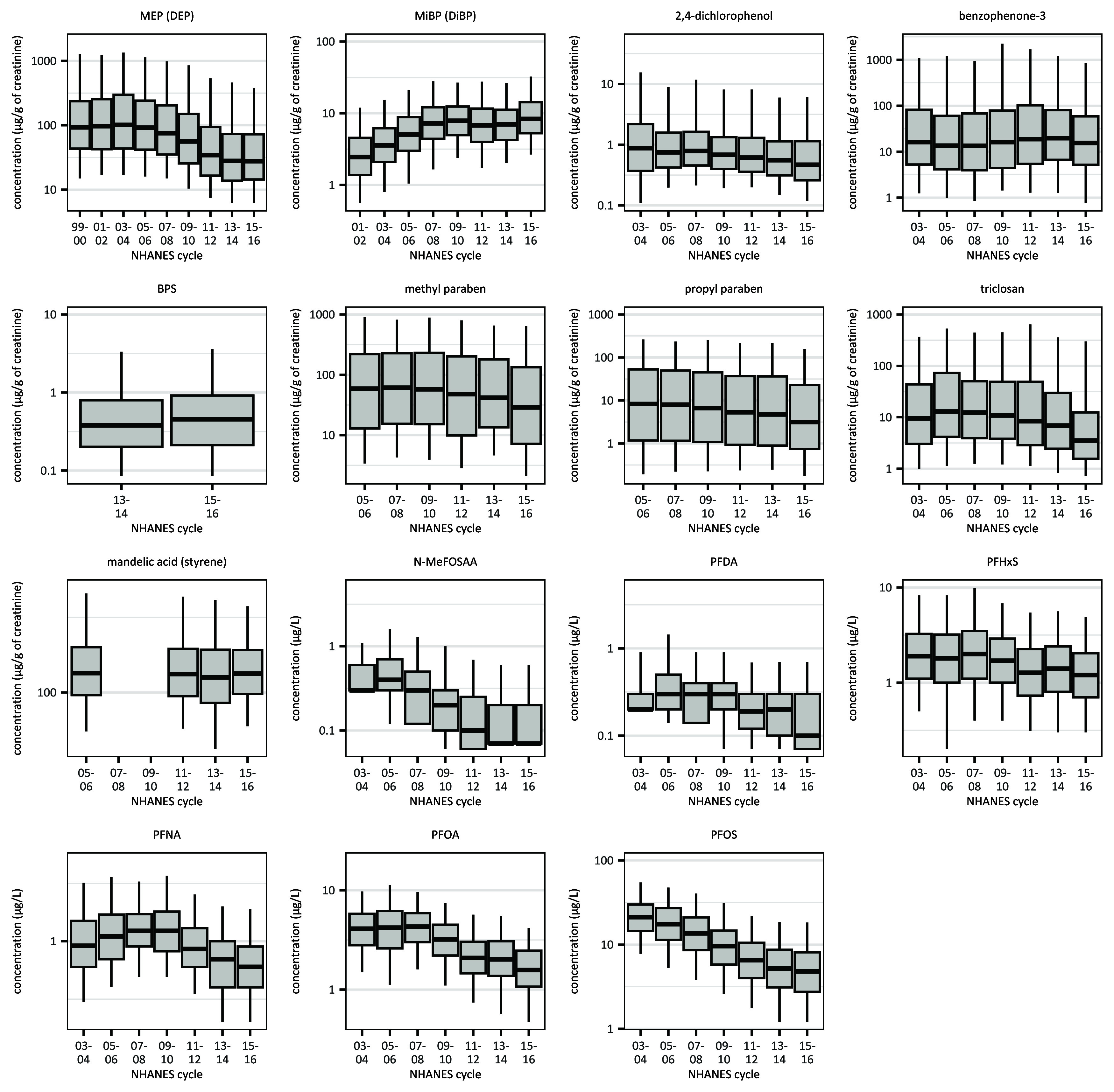
Post-listing, there were significant decreases in concentrations for both Californians and non-Californians for MBzP, MnBP, and MEHHP (Figure 1, Tables 2 and 3; Excel Table S2). There were no significant differences in the magnitude of the decrease for Californians relative to non-Californians (interaction term was not significant). Based on the difference-in-differences results, which compared the pre-listing to post-listing time periods, concentrations of MCOP appear to have increased post-listing (2013) (Table 2). However, looking at the publicly available national-level data, median MCOP concentration increased each cycle from 2005–2006 to 2011–2012, was slightly lower in the 2013–2014 cycle, and then declined by 65% from the 2013–2014 to the 2015–2016 cycle (Figure 2).
Figure 1.
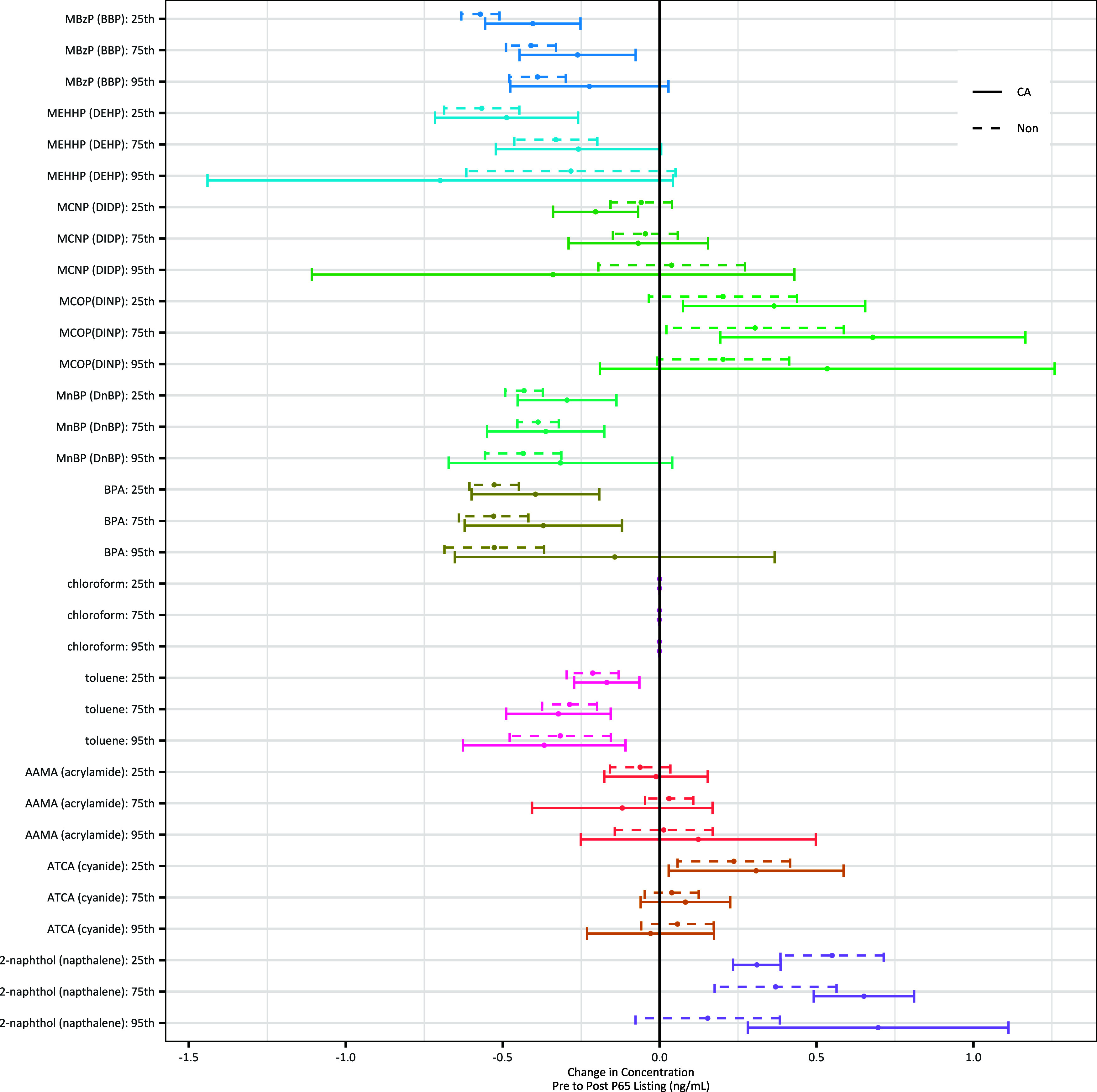
Estimated change (range shows 95% confidence interval) in natural-logged chemical concentrations from pre- to post-Prop 65–listing, for Californians and non-Californians, for the 25th, 75th, and 95th percentiles of the distribution, based on quantile regression models, controlling for demographics, creatinine for chemicals measured in urine, and cotinine for chemicals associated with smoking. Chemicals are those listed on Prop 65 during the biomonitoring period. Underlying data for the figure is contained in Excel Table S2, “Figure 1 Supporting Data” tab. Note: AAMA, -acetyl--(2-carbamoylethyl)-l-cysteine; ATCA, 2-aminothiazoline-4-carboxylic acid; BBP, benzylbutyl phthalate; BPA, bisphenol A; CA, Californian; DEHP, di(2ethylhexyl) phthalate; DIDP, diisodecyl phthalate; DINP, diisononyl phthalate; DnBP, di--butyl phthalate; MBzP, monobenzyl phthalate; MCNP, mono(carboxynonyl) phthalate; MCOP, mono(carboxyoctyl) phthalate; MEHHP, mono-(2-ethyl-5-hydroxyhexyl) phthalate; MnBP, mono--butyl phthalate; Non, non-Californian; Prop 65, Proposition 65.
Figure 2.
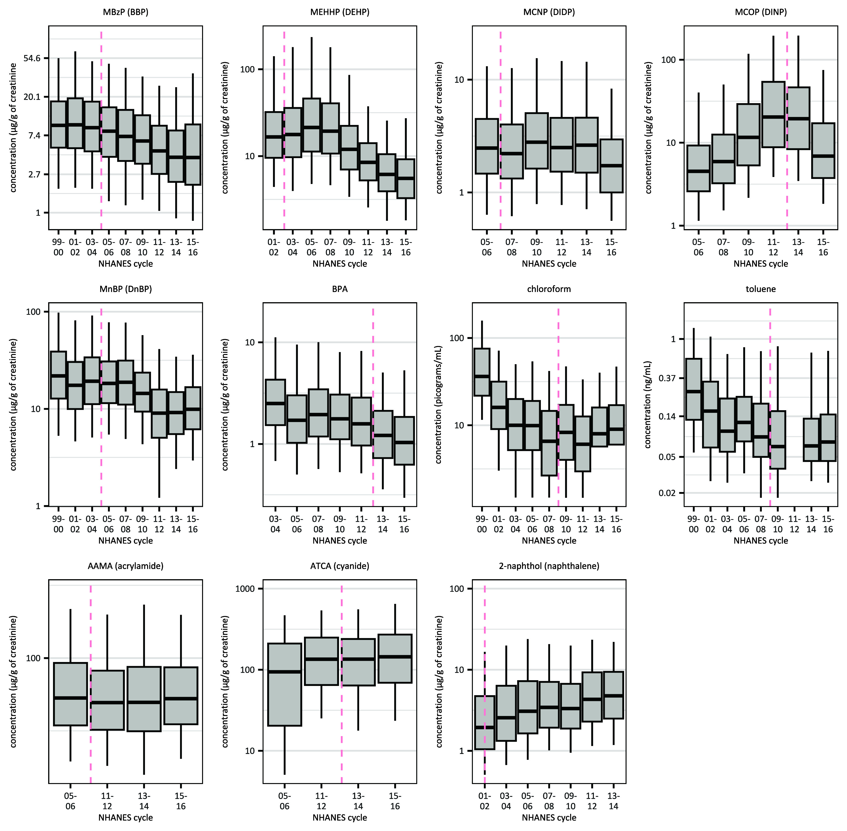
Biomonitored concentrations, for the United States as a whole, for chemicals listed on Prop 65 during the biomonitoring period. NHANES cycle is listed along the x-axis. Box plots represent 5th (lower whisker), 25th (bottom of box), 50th (dark center line), 75th (top of box), and 95th (upper whisker) percentiles of the nationally representative, publicly available data. For chemicals measured in urine, concentrations shown are creatinine-adjusted. Dashed pink line corresponds to the Prop 65 listing date. Underlying data for the figure is contained in Excel Table S3, “Figure 2 Supporting Data” tab. Note: AAMA, -acetyl--(2-carbamoylethyl)-l-cysteine; ATCA, 2-aminothiazoline-4-carboxylic acid; BBP, benzylbutyl phthalate; BPA, bisphenol A; DEHP, di(2ethylhexyl) phthalate; DiDP, diisodecyl phthalate; DINP, diisononyl phthalate; DnBP, di--butyl phthalate; MBzP, monobenzyl phthalate; MCNP, mono(carboxynonyl) phthalate; MCOP, mono(carboxyoctyl) phthalate; MEHHP, mono-(2-ethyl-5-hydroxyhexyl) phthalate; MnBP, mono--butyl phthalate; NHANES, National Health and Nutrition Examination Survey; Prop 65, Proposition 65.
Prior to BPA’s 2013 listing, Californians had significantly lower BPA concentrations than the rest of the nation (Table 2). Post-listing, there were significant decreases for both Californians and non-Californians across the concentration distribution (Figure 1; Excel Table S2). Median BPA concentrations decreased 15% from 2013–2014 to 2015–2016 (Figure 2; Excel Table S3). As with phthalates, the magnitude of the decrease was not statistically different between Californians and non-Californians.
Four chemicals from the VOC panel were listed under Prop 65 during the biomonitoring period: toluene, chloroform, acrylamide, and cyanide. All but cyanide also had earlier listings on Prop 65 for a different health end point. There were no significant differences in mean concentrations between Californians and non-Californians for any of these chemicals prior to their listing (Table 2). This result held across the concentration distribution, with the exception that Californians had significantly higher concentrations of acrylamide than non-Californians at the 25th percentile (Table 3). After listing, concentrations significantly decreased for both Californians and the rest of the US population for chloroform and toluene (Table 2); this decrease from the pre- to post-listing period may be attributable to lower exposures that preceded the second listing (Figure 2; Excel Table S3). Mean concentrations of ATCA (a metabolite of cyanide) significantly increased post-listing for both groups, likely due to changes at the lower half of the exposure distribution in the first cycle it was measured (Figure 2; Excel Table S3).
Concentrations of -acetyl--(2-carbamoylethyl)-l-cysteine (AAMA; a metabolite of acrylamide) did not change significantly post-listing for either group. In all these cases, there was no significant difference in how chemical exposures changed for Californians relative to non-Californians.
One PAH, naphthalene, was listed on Prop 65 during the biomonitoring period. Pre-listing, Californians had significantly lower concentrations of 2-napthol, a metabolite of naphthalene, than the rest of the nation’s population. Concentrations significantly increased post-listing for both Californians and the rest of the United States, across the distribution.
Chemicals Listed Prior to Start of Biomonitoring
We evaluated 13 analytes of 11 chemicals listed on Prop 65 prior to the start of the biomonitoring period. Without data from both before and after Prop-65 listing, we estimated only the differences in Californians vs. non-Californians over the entire time period, as well as concentration changes over time for NHANES participants as a whole. These included 2,5-dichlorophenol, a metabolite of the disinfectant p-DCB. Concentrations of 2,5-dichlorophenol were significantly lower among Californians than for the rest of the nation. 2,5-Dichlorophenol concentrations also significantly decreased over time across the United States (Table 4), with median concentrations decreasing 78% from the 2003–2004 to the 2015–2016 cycle (Figure 3A; Excel Table S4).
Table 4.
Linear and quantile regression results for 13 analytes of 11 chemicals listed before the start of biomonitoring data (1999), for California vs. the rest of the United States over the entire time period (CA) and a time trend (time).
| Chemical | CA | Time | |||||||
|---|---|---|---|---|---|---|---|---|---|
| Mean (95% CI) | 25th % (95% CI) | 75th % (95% CI) | 95th % (95% CI) | Mean (95% CI) | 25th % (95% CI) | 75th % (95% CI) | 95th % (95% CI) | ||
| Phenols | |||||||||
| 2,5-Dichlorophenol (p-DCB) | 16,822 | (, ) | (, ) | (, ) | (, ) | (, ) | (, ) | (, ) | (, ) |
| VOCs | |||||||||
| DHBMA (1,3-butadiene) | 9,496 | 0.03 (, 0.1) | 0.05 (, 0.2) | 0.001 (, 0.05) | 0.07 (, 0.2) | 0.02 (0.01, 0.03) | 0.02 (0.02, 0.03) | 0.01 (0.009, 0.02) | 0.01 (0.000008, 0.02) |
| MHBMA3 (1,3-butadiene) | 9,652 | 0.04 (, 0.2) | 0.08 (, 0.2) | 0.1 (0.02, 0.2) | 0.06 (, 0.2) | (, ) | (, 0.005) | (, ) | (, 0.008) |
| CYMA (acrylonitrile) | 9,698 | 0.1 (0.01, 0.3) | 0.1 (0.06, 0.2) | (, 0.1) | 0.1 (, 0.5) | 0.0009 (, 0.01) | (, 0.009) | 0.01 (0.001, 0.03) | 0.05 (0.02, 0.08) |
| 2HPMA (propylene oxide) | 9,719 | 0.06 (, 0.1) | 0.04 (, 0.2) | 0.1 (, 0.2) | 0.2 (, 0.5) | (, ) | (, ) | (, ) | (, 0.02) |
| 3MHA + 4MHA (xylene) | 9,740 | 0.03 (, 0.1) | 0.1 (0.02, 0.2) | 0.02 (, 0.2) | (, 0.07) | (, ) | (, ) | 0.007 (, 0.02) | (, 0.0002) |
| PAHs | |||||||||
| 2-Hydroxyfluorene (fluorene) | 15,629 | (, ) | (, ) | (, ) | (, ) | (, ) | (, ) | (, ) | (, ) |
| 1-Hydroxyphenanthrene (phenanthrene) | 15,636 | (, ) | (, ) | (, ) | (, ) | (, ) | (, ) | (, ) | (, ) |
| 3-Hydroxyphenanthrene (phenanthrene) | 13,285 | (, ) | (, ) | (, ) | (, ) | (, ) | (, ) | (, ) | (, ) |
| 1-Hydroxypyrene (pyrene) | 15,600 | (, ) | (, ) | (, ) | (, ) | 0.09 (0.08, 0.09) | 0.09 (0.09, 0.1) | 0.08 (0.07, 0.08) | 0.06 (0.04, 0.07) |
| Metals | |||||||||
| Cadmium | 20,066 | 0.09 (0.04, 0.1) | 0.09 (0.007, 0.2) | 0.09 (0.03, 0.2) | 0.04 (, 0.1) | (, ) | (, ) | (, ) | (, ) |
| Lead | 63,592 | (, ) | (, ) | (, ) | (, ) | (, ) | (, ) | (, ) | (, ) |
| Mercury | 53,039 | 0.2 (0.1, 0.3) | 0.2 (0.03, 0.3) | 0.2 (0.08, 0.4) | 0.1 (0.03, 0.2) | (, ) | (, ) | (, ) | (, ) |
Note: Linear and quantile regression results (effect estimates and 95 percentile CIs) for chemicals listed before the start of the biomonitoring data. CA represents binary indicator of California vs. rest of the United States and time represents integer year (0,1,2, and so on) since the beginning of the available data. The estimated coefficient on CA represents the difference in Californians’ concentrations relative to the rest of the United States over the entire time period, whereas the estimated coefficient on the time trend represents the change over time for the entire population. All regression models include the following covariates whose coefficient estimates are not reported: female (0/1), child (0/1; equal to 1 for participants of age), female of childbearing age ( for females 18–50 years of age), race/ethnicity [coded as Hispanic (combining Mexican American and Other Hispanic RIDRETH1 categories), Non-Hispanic White, Non-Hispanic Black, and Other (including Asian)], and federal poverty level [total family income divided by the poverty threshold, with participants categorized as low income (), moderate income (), and high income ()]. For metabolites measured in urine, we included ln(creatinine) as a covariate to account for urinary dilution. For chemicals associated with smoking, we controlled for smoking status by including ln(cotinine) as a covariate. %, Percentile; 2HPMA, n-acetyl-S-(2-hydoxypropyl)-L-cysteine; 3MHA, 3-methylhippuric acid; 4MHA, 4-methylhippuric acid; CI, confidence interval; CYMA, -acetyl--(2-cyanoethyl)-l-cysteine; DHBMA, -acetyl--(3,4-dihidroxybutyl)-l-cysteine; FPL, federal poverty level; MHBMA3, -acetyl--(4-hydroxy-2-butenyl)-l-cysteine; PAH, polycyclic aromatic hydrocarbon; RIDRETH1, race/ethnicity variable that can be linked to the corresponding variable from NHANES 1999–2010; VOC, volatile organic compound.
Figure 3.
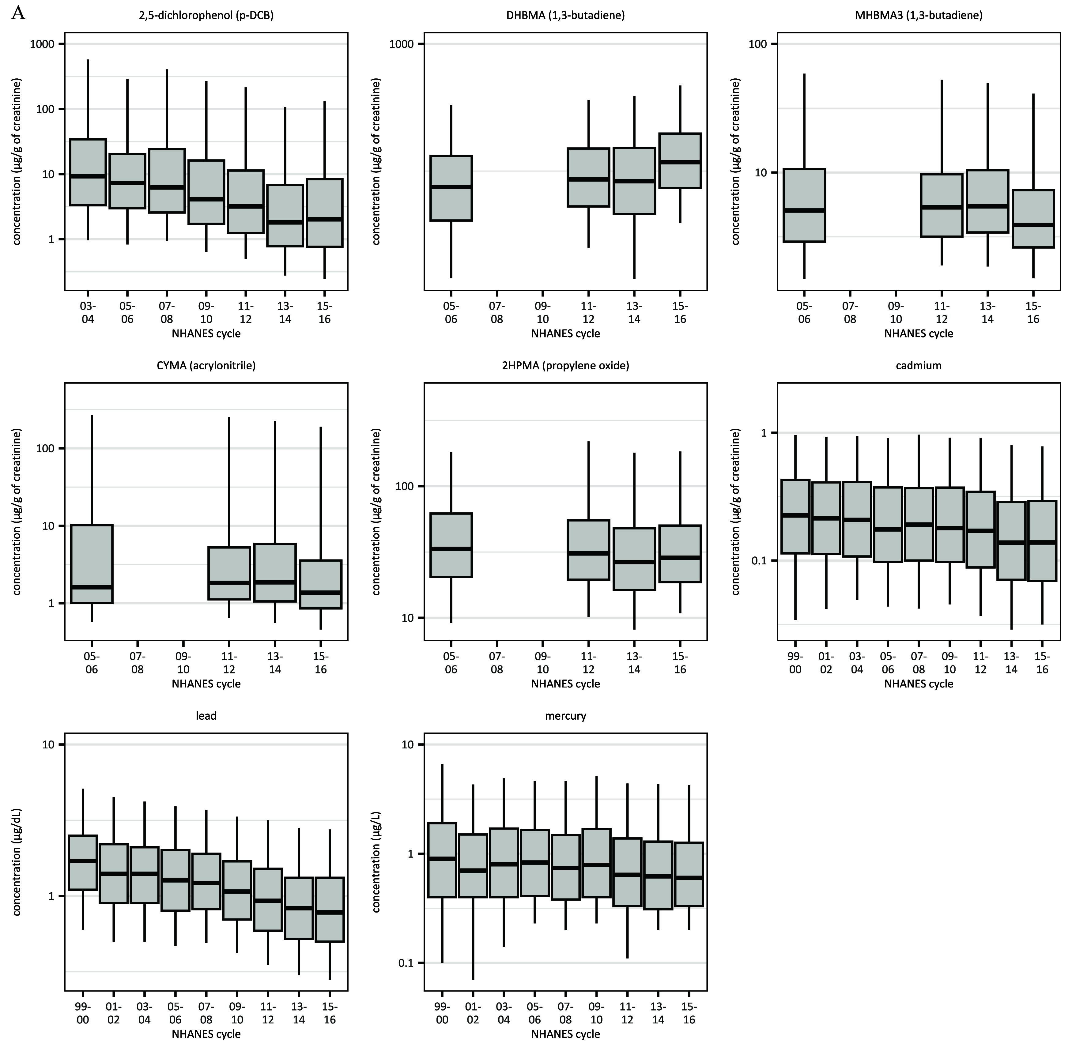
Biomonitored concentrations, for the United States as a whole, for chemicals listed before 1999 (start of NHANES data). NHANES cycle is listed along the x-axis. Box plots represent 5th (lower whisker), 25th (bottom of box), 50th (dark center line), 75th (top of box), and 95th (upper whisker) percentiles of the nationally representative, publicly available data for (A) non–diesel-related and (B) diesel-related chemicals. For chemicals measured in urine, concentrations shown are creatinine-adjusted. Underlying data for the figure is contained in Excel Tables S4 and S5, “Figure 3a Supporting Data” and “Figure 3b Supporting Data” tabs. Note: 2HPMA, n-acetyl-S-(2-hydroxypropyl)-L-cysteine; 3MHA, 3-methylhippuric acid; 4MHA, 4-methylhippuric acid; CYMA, -acetyl--(2-cyanoethyl)-l-cysteine; DHBMA, -acetyl--(3,4-dihidroxybutyl)-l-cysteine; MHBMA3, -acetyl--(4-hydroxy-2-butenyl)-l-cysteine; NHANES, National Health and Nutrition Examination Survey; p-DCB, -dichlorobenzene.
Three heavy metals—lead, cadmium, and mercury—were listed on Prop 65 before the biomonitoring period. Californians had significantly lower lead concentrations, but higher concentrations of cadmium and mercury, than the rest of the United States. Concentrations of all three metals significantly decreased over time across the United States (Table 4): Median lead concentrations decreased 54%, and cadmium concentrations decreased 39% from the 1999–2000 to the 2015–2016 cycle (Figure 3A; Excel Table S4).
Three VOCs—acrylonitrile, 1,3-butadiene, and propylene oxide—were listed on Prop 65 prior to the start of the biomonitoring period. Californians had significantly higher concentrations of -acetyl--(2-cyanoethyl)-l-cysteine (CYMA; a metabolite of acrylonitrile) compared with those living outside California (Table 4). Concentrations were not significantly different between Californians and non-Californians for DHBMA and MHBMA3 (both metabolites of 1,3-butadiene) or for 2-hydroxypropyl methacrylate (2HPMA; a metabolite of propylene oxide). Concentrations of 2HPMA decreased significantly nationwide over time. Concentrations of CYMA increased significantly over time at the upper end of the exposure distribution only. Time trends for the two 1,3-butadiene metabolites, DHBMA and MHBMA3, moved in opposite directions: DHBMA concentrations increased significantly across the distribution, and MHBMA3 concentrations—which are most closely correlated with tobacco smoking—decreased significantly (Table 4).
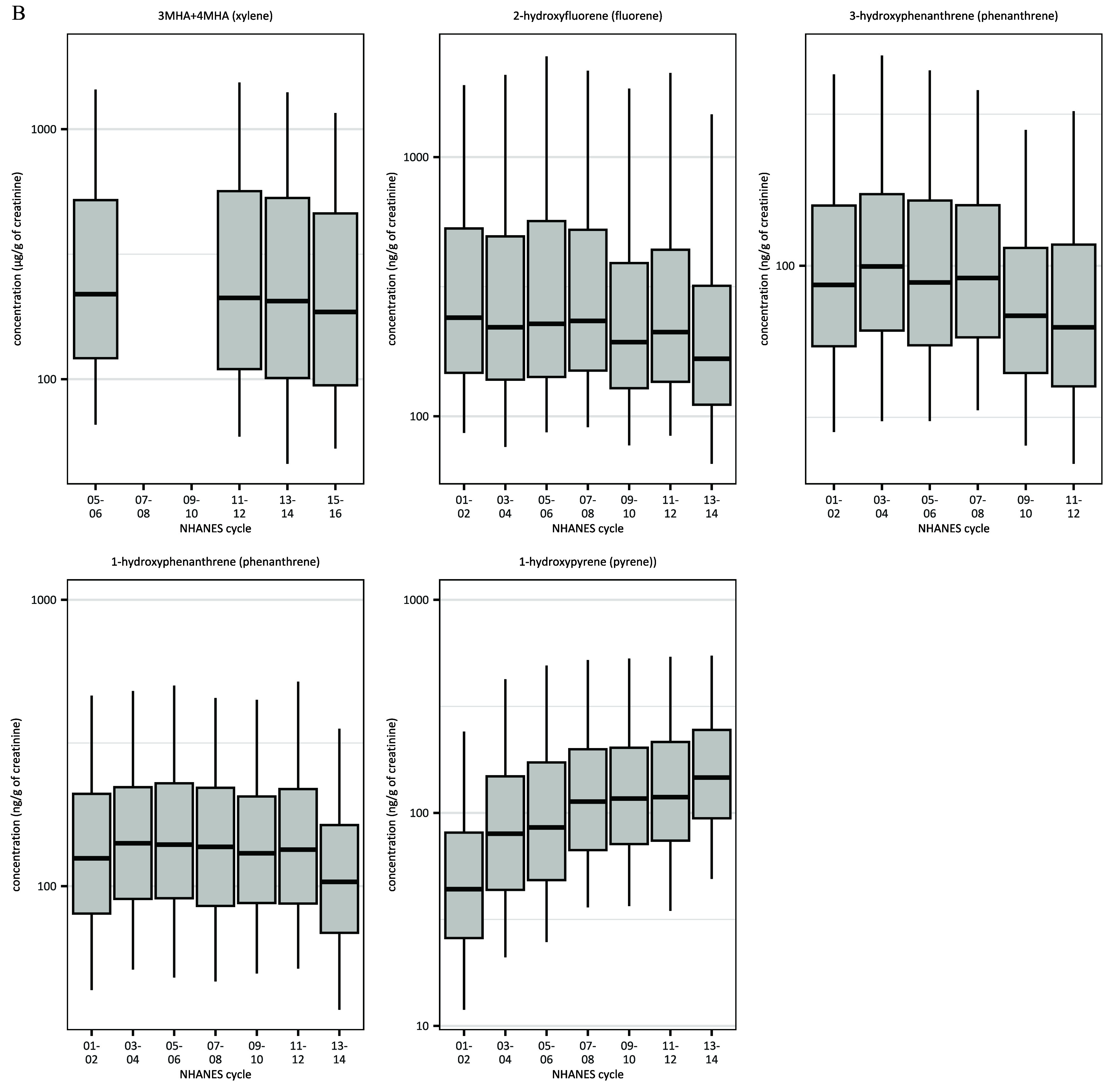
Diesel engine exhaust was listed on Prop 65 in 1990, before the biomonitoring program began. Throughout the window of available biomonitoring data, concentrations of the diesel-related PAH metabolites 2-hydroxyfluorene, 1-hydroxyphenanthrene, 3-hydroxyphenanthrene, and 1-hydroxypyrene were significantly lower in Californians than in the rest of the US population. Although concentrations of 2-hydroxyfluorene, 1-hydroxyphenanthrene, and 3-hydroxyphenanthrene significantly decreased over time, concentrations of 1-hydroxypyrene significantly increased (Figure 3B; Excel Table S5). Concentrations of 3MHA + 4MHA (the sum of two metabolites of xylene), a VOC that is related to diesel but also appears in industrial solvents, were overall not significantly different in Californians than in non-Californians and decreased over time.
Chemicals Not Listed Within Biomonitoring Window
To provide context for our analysis of listed chemicals, we also examined 15 chemicals that were included in the analytical panels for phthalates, phenols, VOCs, and PFAS but that were not listed under Prop 65 during the window for which biomonitoring data were available, although 4 were subsequently listed (Table 5). For the 2 nonlisted phthalates, Californians, on average, had significantly lower levels of monoethyl phthalate (MEP, a metabolite of DEP) than the rest of the US population, but there was no difference in levels of MiBP (a metabolite of DiBP) (Table 5). Concentrations of MEP decreased over time, whereas concentrations of MiBP increased over time. Median levels of MiBP increased 240% from the 2001–2002 cycle to the 2015–2016 cycle (Figure 4; Excel Table S6).
Table 5.
Linear and quantile regression results for 15 chemicals not listed as of the end of the biomonitoring period (2016), for California vs. the rest of the United States over the entire time period (CA) and a time trend (time).
| Chemical | CA | Time | |||||||
|---|---|---|---|---|---|---|---|---|---|
| Mean (95% CI) | 25th % (95% CI) | 75th % (95% CI) | 95th % (95% CI) | Mean (95% CI) | 25th % (95% CI) | 75th % (95% CI) | 95th % (95% CI) | ||
| Phthalates | |||||||||
| MEP (DEP) | 22,006 | (, ) | (, ) | (, ) | (, 0.1) | (, ) | (, ) | (, ) | (, ) |
| MiBP (DiBP) | 19,797 | 0.007 (, 0.09) | 0.0007 (, 0.1) | 0.02 (, 0.1) | (, 0.1) | 0.08 (0.07, 0.08) | 0.08 (0.07, 0.09) | 0.07 (0.06, 0.07) | 0.06 (0.05, 0.07) |
| Phenols | |||||||||
| 2,4-Dichlorophenol | 16,822 | (, ) | (, ) | (, ) | (, 0.07) | (, ) | (, ) | (, ) | (, ) |
| Benzophenone-3 | 16,815 | 0.1 (, 0.3) | 0.1 (, 0.3) | 0.05 (, 0.3) | 0.03 (, 0.3) | 0.02 (0.002, 0.03) | 0.03 (0.01, 0.05) | 0.01 (, 0.03) | 0.01 (, 0.04) |
| BPS | 4,847 | (, 0.05) | (, 0.03) | (, 0.2) | (, 0.6) | 0.03 (, 0.1) | 0.01 (, 0.08) | 0.1 (0.02, 0.2) | (, 0.2) |
| Methyl paraben | 14,426 | 0.03 (, 0.2) | 0.001 (, 0.2) | (, 0.1) | 0.006 (, 0.3) | (, ) | (, ) | (, ) | (, ) |
| Propyl paraben | 14,426 | 0.09 (, 0.3) | 0.02 (, 0.2) | 0.1 (, 0.4) | 0.1 (, 0.4) | (, ) | (, ) | (, ) | (, 0.009) |
| Triclosan | 16,815 | 0.06 (, 0.3) | (, 0.08) | 0.3 (, 0.7) | 0.2 (, 0.4) | (, ) | (, ) | (, ) | (, ) |
| VOCs | |||||||||
| Mandelic acid (styrene) | 9,668 | 0.06 (0.02, 0.1) | — | 0.02 (, 0.08) | (, 0.2) | (, 0.004) | — | 0.002 (, 0.009) | 0.0005 (, 0.01) |
| PFAS | |||||||||
| N-MeFOSAA | 13,432 | (, ) | (, 0.007) | (, ) | (, 0.1) | (, ) | (, ) | (, ) | (, ) |
| PFDA | 13,432 | (, 0.006) | (, 0.07) | (, ) | (, ) | (, ) | (, ) | (, ) | (, ) |
| PFHxS | 13,432 | (, ) | (, 0.02) | (, 0.005) | (, ) | (, ) | (, ) | (, ) | (, ) |
| PFNA | 13,432 | (, ) | (, 0.05) | (, ) | (, ) | (, ) | (, ) | (, ) | (, ) |
| PFOA | 13,430 | (, ) | (, ) | (, ) | (, ) | (, ) | (, ) | (, ) | (, ) |
| PFOS | 13,430 | (, ) | (, ) | (, ) | (, ) | (, ) | (, ) | (, ) | (, ) |
Note: Linear and quantile regression results (effect estimates and 95 percentile CIs) for chemicals either not listed or listed after the end of the biomonitoring data. CA represents binary indicator of California vs. rest of United States and time represents integer year (0,1,2, and so on) since the beginning of the available data. The estimated coefficient on CA represents the difference in Californians’ concentrations relative to the rest of the United States over the entire time period, whereas the estimated coefficient on the time trend represents the change over time for the entire population. All regression models include the following covariates whose coefficient estimates are not reported: female (0/1), child (0/1; equal to 1 for participants of age), female of childbearing age ( for females 18–50 years of age), race/ethnicity [coded as Hispanic (combining Mexican American and Other Hispanic RIDRETH1 categories), Non-Hispanic White, Non-Hispanic Black, and Other (including Asian)], and federal poverty level [total family income divided by the poverty threshold, with participants categorized as low income (), moderate income (), and high income ()]. For metabolites measured in urine, we included ln(creatinine) as a covariate to account for urinary dilution. For chemicals associated with smoking, we controlled for smoking status by including ln(cotinine) as a covariate. —, Not available; %, percentile; BPS, bisphenol S; CI, confidence interval; DEP, diethyl phthalate; DiBP, di-isobutyl phthalate; FPL, federal poverty level; MEP, monoethyl phthalate; MiBP, monoisobutyl phthalate; N-MeFOSAA, 2-(-methyl-perfluorooctane sulfonamido)acetic acid; PFAS, per- and polyfluoroalkyl substances; PFDA, pefluorodecanoic acid; PFHxS, perfluorohexane sulfonic acid; PFNA, perfluorononanoic acid; PFOA, perfluorooctanoic acid; PFOS, perfluorooctane sulfonic acid; RIDRETH1, race/ethnicity variable that can be linked to the corresponding variable from NHANES 1999–2010; VOC, volatile organic compound.
Figure 4.
Biomonitored concentrations, for the United States as a whole, for chemicals not listed on Prop 65 as of the end of the biomonitoring period. NHANES cycle is listed along the x-axis. Box plots represent 5th (lower whisker), 25th (bottom of box), 50th (dark center line), 75th (top of box), and 95th (upper whisker) percentiles of the nationally representative, publicly available data. For chemicals measured in urine, concentrations shown are creatinine-adjusted. Underlying data for the figure is contained in Excel Table S6, “Figure 4 Supporting Data” tab. Note: BPS, bisphenol S; DEP, diethyl phthalate; DiBP, diisobutyl phthalate; MEP, monoethyl phthalate; MiBP, monoisobutyl phthalate; NHANES, National Health and Nutrition Examination Survey; N-MeFOSAA, 2-(-methyl-perfluorooctane sulfonamido)acetic acid; PFDA, pefluorodecanoic acid; PFHxS, perfluorohexane sulfonic acid; PFNA, perfluorononanoic acid; PFOA, perfluorooctanoic acid; PFOS, perfluorooctane sulfonic acid; Prop 65, Proposition 65.
Among nonlisted phenolic compounds common in consumer products, Californians had significantly lower levels of 2,4-dichlorophenol than the rest of the nation across the concentration distribution, but there was no geographic difference in the observed concentrations of benzophenone-3, BPS, methyl paraben, propyl paraben, or triclosan. Concentrations of 2,4-dichlorophenol, methyl paraben, propyl paraben, and triclosan decreased significantly over time. Benzophenone-3 and BPS concentrations increased over time. Median concentrations of BPS increased 20% from 2013–2014 to 2015–2016 (Figure 4; Excel Table S6). For the one nonlisted VOC in this group, styrene, Californians had significantly higher mean concentrations of its metabolite, mandelic acid, than the population of the rest of the United States, and concentrations did not change significantly over time in either population.
Californians had significantly lower concentrations of the six nonlisted PFAS than did residents in the rest of the nation. This was the case for PFOA and PFOS across the concentration distribution and for other nonlisted PFAS at the upper ends of the distribution (Table 5). Concentrations of all six PFAS (N-MeFOSAA, PFDA, PFHxS, PFNA, PFOA, and PFOS) significantly decreased over time across the distribution. Median levels decreased by 77% for both PFOS and N-MeFOSAA, and 62% for PFOA.
Sensitivity Analysis
To check the effect of creatinine correction on our analysis, we estimated regression models for chemical metabolites measured in urine with and without ln(creatinine) as a covariate. The results were generally consistent (Tables S1–S4).
Discussion
Understanding changes in body burdens of chemicals targeted by regulation can inform the design of chemicals policy, as well as the structure of biomonitoring programs that might detect the impacts of policy interventions. We evaluated the impact of Prop 65 because it covers hundreds of toxic chemicals in a wide variety of uses, and it has proven particularly relevant in reducing chemical exposures from consumer products.54,55 Our goals were to learn how Prop 65 in particular might have affected exposure to toxic chemicals in California and nationwide; to identify data limitations that might preclude definitive answers to the question, Are toxics reduction policies reducing human exposure?; and to consider how surveillance biomonitoring could better show the effects of toxics policy.
To assess the relationship between chemical listings under California’s Prop 65 and trends in population-level exposures to those chemicals in California and the rest of the country, we analyzed NHANES biomonitoring data on chemical concentrations in both groups, comparing distributions in the population and trends over time. We investigated whether the addition of a chemical to the Prop 65 list was followed by changes in urinary or blood measurements of that chemical’s metabolites among residents of California compared with residents of the rest of the United States.
Many factors influence population-level exposures to toxic chemicals, including regulatory pressure at international, federal, or state levels (in addition to Prop 65 listing); consumer and retailer campaigns targeting specific chemicals or product categories; enforcement actions under Prop 65 or other chemical laws; and changes in business marketing or consumer behaviors, such as product use and purchasing decisions unrelated to policy. We interpreted our findings within the context of this web of interrelated factors that drive changes in exposure to chemicals over time.
Trends in Chemical Concentrations Over Time for Prop 65 Listed Chemicals
Exposures to chemicals included in the NHANES biomonitoring program would be expected to decline over time because a chemical’s inclusion in the program is typically associated with concern about its health effects. Declines may be due to direct regulation, voluntary chemical deselection by producers, chemical avoidance by users, or all three reasons.22,37,56 Our findings for chemicals listed under Prop 65, as well as unlisted chemicals, support this conclusion. Concentrations declined nationwide over time for 8 of 11 chemicals listed on Prop 65 before the biomonitoring period, including lead, cadmium, mercury, 2,5-dichlorophenol, 2HPMA (a metabolite of propylene oxide), and metabolites of the diesel-related chemicals fluorene, phenanthrene, and xylene. Concentrations declined nationwide after Prop 65 listing for 6 of 11 chemicals listed during the biomonitoring period: the phthalate metabolites (MBzP, MEHHP, and MnBP), BPA, chloroform, and toluene. For the phthalate metabolite MCOP, concentrations rose prior to listing and fell afterward. For chemicals not listed under Prop 65, concentrations of 11 of 15 chemicals likewise decreased over time across the country. Our data also confirmed previous findings that few biomonitored chemicals increased in concentration over time.57,58
This general downward exposure trend suggests relationships among multiple regulatory and nonregulatory forces, including but by no means limited to Prop 65. Further, biannual publication of national exposure data on specific chemicals, and the media campaigns and coverage this reporting generates, may itself prompt regulators, businesses, and individuals to take actions that reduce exposure.59 Thus, exposure to biomonitored chemicals may be becoming less prevalent specifically because of the attention that biomonitoring generates. These factors, particularly when combined with the lack of biomonitoring data for most Prop 65-listed chemicals, make it difficult to isolate the influence of Prop 65 on exposures.
In a few specific instances, Prop 65 appears very likely to have influenced exposures. For example, DEHP’s listing was followed by considerable, highly publicized Prop 65 enforcement litigation,60 as well as attention from media, civil society, and the legislature regarding the chemical’s toxicity and ubiquity.7 These direct and indirect effects of Prop 65 listing clearly prompted market deselection as companies settled cases by agreeing to reformulate DEHP-containing products, and California imposed limits on some uses of DEHP.
In other instances, decreasing exposures over time are probably unrelated to Prop 65 listing. For example, concentrations of MEP began dropping in 2007, even though its parent compound, DEP, has never been listed under Prop 65. Complicating the story, since the mid–2000s, phthalates as a class have been restricted by legislation in states beyond California, as well as at the national and international level.61–63 Phthalates as a chemical class have also been targeted by advocacy campaigns that encourage consumers and retailers to avoid them altogether.26
Declining concentrations of certain PFAS over the biomonitoring period are also unlikely to be related to Prop 65, which listed chemicals from this class only after the biomonitoring window. Observed changes may be attributable to a combination of tort litigation,64 local and state legislation, media coverage of accumulating scientific evidence, and the US Environmental Protection Agency’s (EPA) negotiations with industry to voluntarily phase out PFOA and PFOS.65 Similarly, decreases in levels of methyl and propyl paraben cannot be attributed to Prop 65, which does not list either chemical. Parabens—endocrine disruptors used as preservatives in personal care products—have been stigmatized by many consumer campaigns, which are especially effective at targeting chemicals that (like parabens) are included on ingredient labels.66 Taken together, these examples point to the many regulatory and nonregulatory forces that drive changes in population-level chemical exposures.
For a small number of biomonitored Prop 65 chemicals, concentrations increased after Prop 65 listing. Concentrations of 2-naphthol (metabolite of naphthalene) increased following listing (Figure 2; Excel Table S3), although our analysis is limited by the single year of pre-listing data for naphthalene. Our findings are consistent with another recent analysis of NHANES data showing this naphthalene metabolite increasing over time across the United States.67 There are many anthropogenic and natural sources of naphthalene: It is released by diesel combustion, industrial processes, building materials, fumigants, and household pesticides, as well as wildfires.68,69 The major contributors to (nonoccupational) naphthalene exposure are now indoors, including the use of moth repellents, the presence of an attached garage, and some common building products, such as vinyl and foam-based home products, caulking, carpet pads, and rubber floor covering.67,68,70 Although indoor concentrations of many volatile consumer product chemicals have decreased over time, levels of naphthalene have not.68
One of the 1,3-butadiene metabolites (DHBMA) also increased in the most recent monitoring period, whereas the other (MHBMA3) decreased. The sources associated with the increase are unclear, although butadiene exposure is generally attributed to vehicle exhaust, tobacco smoking, and other combustion-related sources,71 or occupational settings with synthetic rubber (styrene–butadiene rubber). 1,3-Butadiene has been detected in air near fires,72 and its metabolite, MHBMA3, increased in firefighters after firefighting activities.73 MHBMA3 has been associated with tobacco smoking,74 whereas DHBMA has been associated with vaping.75
Exposure Trends for Chemicals Closely Related to Prop 65 Listed Chemicals
Despite decreasing exposures to many biomonitored chemicals irrespective of Prop 65 listing, we also saw changing patterns of exposure to certain chemical pairs that reflect likely chemical substitutions in products and suggest a driving role of Prop 65. For example, the pattern of phthalate concentrations over time suggests manufacturers may replace Prop 65-listed chemicals in this class with closely related chemicals that are not Prop 65-listed. We found decreasing concentrations of MnBP (a metabolite of DnBP) after DnBP was listed in 2005 at the same time as concentrations increased for metabolites of the closely related but unlisted phthalate DiBP (Figures 2 and 4).
Similarly, we observed a significant decrease in MEHHP (a DEHP metabolite) after DEHP’s listing in 2003 (Table 2) but saw concentrations of MCOP (a metabolite of DiNP) increase concurrently. This is consistent with evidence that then-unlisted DiNP served as a substitute for DEHP.76 MCOP concentrations then decreased after DiNP was listed in 2013 (Figure 2; Excel Table S3). The difference-in-differences model showing higher concentrations of MCOP post-listing for Californians relative to the rest of the country (Table 2) likely reflects the fact that the difference-in-differences model groups years together into pre- and post-listing buckets, as well as the overlap between the period designated as post-listing in our model and the actual period of reformulation: reformulation might occur in the year post-listing, which is a transition period before manufacturers face a legal obligation to warn, and is also a time when existing inventory can be sold without warning.10
In a parallel finding, we saw concentrations of BPA decrease after the chemical’s Prop 65 listing in 2013, whereas concentrations of (unlisted) BPS increased. BPS is known to substitute for BPA in such common products and applications as polycarbonate plastic bottles, thermal receipt paper, and epoxy resin food can linings.77 Other researchers have found increasing concentrations of both BPS and the also-unlisted, closely related biphenyl bisphenol F (BPF) in US pregnant women from 2006 through 2019.78
California Levels vs. the Rest of the Nation
Where we had both pre- and post-listing biomonitoring data and could thus estimate difference-in-differences models, we observed parallel time trends for concentrations of Prop 65 chemicals in Californians and the population in the rest of the United States. This mirrors our findings from interviews with manufacturers, who reported that when Prop 65 prompts them to reformulate products, practical and legal considerations typically induce them to do so on a nationwide basis.7
One particularly intriguing result with implications for understanding policy impacts was our finding that Californians had significantly lower concentrations than residents of other states for about half of the chemicals we examined. At the mean, levels in Californians were significantly lower for 18 of the 37 biomonitored chemicals, whereas levels in Californians were significantly higher for only 4 chemicals. Californians had significantly lower concentrations for roughly the same proportion of Prop 65 chemicals as nonlisted chemicals.
Californians had lower concentrations than the rest of the US population for many of the diesel-related chemicals included in this study: toluene, fluorene, phenanthrene, pyrene, and naphthalene. Californians also had lower levels of three of the five phthalates; BPA; 2-napthol; 2,5-dichlorophenol; lead; 2,4-dichlorophenol; and all of the PFAS. Californians only had higher mean concentrations than the rest of the US population for styrene, acrylonitrile, cadmium, and mercury.
These geographic trends in exposure have in some cases been linked to California’s regulatory environment and, in other cases, to state-specific demographic and behavioral factors. In the case of exposure to diesel-related chemicals, for example, our previous research describes a series of California policies that sharply reduced the state’s diesel emissions and likely drove the California vs.-non-California differential.79 Diesel exhaust was listed as a carcinogen under Prop 65 in 1990, and many subsequent policy actions by the California Air Resources Board reduced diesel emissions in the state by 78% between 1990 and 2014.79 California’s rules set the state on a different path than the rest of the country such that by 2014, diesel engines in California were producing less than half the emissions than would be expected if the state had followed the same trajectory as the rest of the nation.79 Our data suggests that these policy changes are in turn reflected in lower population exposures to diesel-related chemicals in California than in the rest of the United States.
With respect to mercury, fish consumption is known to drive exposure, and fish consumption is higher in California than in noncoastal areas of the United States.80 In addition, California’s heavy historical use of mercury in mining continues to contaminate surface waters,81 creating additional routes of exposure. For other chemicals, however, differences between Californians’ and non-Californians’ exposure patterns await further investigation. This suggests a ripe and policy-relevant area for further research.
Limitations
For all but a few chemicals we examined, data limitations made it difficult to determine whether Prop 65 directly or indirectly drove observed exposure patterns. One reason is that although NHANES is the largest and most comprehensive source of biomonitoring data in the United States, it includes only a fraction of Prop 65-listed chemicals. For the majority of the chemicals on the Prop 65 list, there are no biomonitoring surveillance data, so exposure trends cannot be established.
Further, for the Prop 65-listed chemicals that are biomonitored, many were listed before the biomonitoring program started, such that baseline concentrations in the US population are unknown. In addition, even for chemicals with NHANES data from pre- and post-listing periods, our analysis may not have been able to detect exposure changes that did occur. For example, levels of the phthalate metabolite MCOP declined considerably in the latest biomonitoring cycle compared with earlier cycles, but the single cycle of biomonitoring data following Prop 65 listing was insufficient for a difference-in-differences analysis.
An additional source of uncertainty in our analysis is the lack of exclusive correspondence between some Prop 65-listed chemicals and NHANES analytes, including metabolites. For example, mandelic acid is considered a biomarker of exposure for the Prop 65 chemical styrene, but it can also signal exposure to ethylbenzene, creating ambiguity in interpretation.30,82 Similarly, two metabolites of 1,3-butadiene (DHBMA and MHBMA3) likely reflect multiple and potentially different exposure sources (including tobacco use and vaping), and the time trends for these two metabolites move in opposite directions. In instances of imperfect correspondence between parent compound and metabolite, research to develop robust biomarkers could enable monitoring of more specific analytes. In addition, differences in biological half-lives determine how quickly biomonitored concentrations reflect changes in exposures; for example, changes in exposure will take longer to be reflected in biomonitoring data of chemicals with relatively long biological half-lives (e.g., PFAS).
For analytes measured in urine, correcting for urine dilution can introduce additional uncertainty. Although potentially more accurate measures of urine dilution are emerging (e.g., urine osmolality, urinary flow rate),83 creatinine was the only measure consistently available in all biomonitoring cycles.
To understand time trends and geographical variations in exposures for people at the extremes of the concentration distributions, we used quantile regression to expand our analyses beyond the mean. Although there were differences across the concentration distribution, small sample sizes in the highest percentiles limited statistical power, and thus, our ability to detect effects in those groups. Future studies focused on more highly exposed subgroups or including larger sample sizes could address this issue.
Finally, our research has two limitations also relevant to future researchers. First, NHANES is not designed to assess exposures at the state level. Indeed, NHANES’ sample—intended to be nationally representative—is collected from just 15 locations each year, such that most states are not sampled in every cycle. This means that the data lack the geographic resolution necessary to provide representative data from any state other than California (which is sampled every cycle). Second, framing data queries acceptable to the RDC and processing them in collaboration with RDC staff is an elaborate, multi-month process. This makes it difficult to engage in iterative research if the results of initial analyses generate new questions.
Implications
Chemicals policy.
Our findings suggest several cases where Prop 65 appears to have prompted manufacturers to deselect specific toxic chemicals, whether by substituting other chemicals, reducing the concentration of the listed chemical, or redesigning products to obviate the need for the toxic chemical’s function. We observed this most clearly for BPA, chloroform, toluene, and three phthalates. Further, in these and other cases where Prop 65 appears to have reduced exposures, our findings indicate that it has done so nationwide, rather than only in California. These data reflect what companies report when interviewed: When reformulating to avoid Prop 65 chemicals, they do so for all products, not only for those sold in California.7 We also observed that exposure to the specific toxic chemicals monitored through NHANES has been generally decreasing over time nationwide, irrespective of whether chemicals are Prop 65-listed.
Our research additionally makes evident that widespread human exposure persists to even those toxic chemicals monitored through NHANES, and further, to even that subset additionally listed under Prop 65. Although relating exposure levels to health outcomes is beyond the scope of this analysis, multiple Prop 65 chemicals (e.g., lead, PFAS) are known to have no safe exposure level,84,85 making enduring exposures over time concerning.
Furthermore, even in cases where manufacturers deselected Prop 65-listed chemicals, the exposure patterns that we saw add to evidence that some replacements are unlisted but still problematic, as with BPA’s substitution with close relatives BPS and BPF, and DEHP’s replacement with DiNP. Substitutions of listed chemicals with similarly problematic chemicals undermines the net health benefits of some chemical-specific restrictions and illustrates the need for chemical policies that address groups of closely related chemicals as classes.86–88 Regulation could also constrain chemical substitution by requiring businesses to use safer alternatives whenever they reduce or eliminate use of regulated chemicals. Although some recently enacted toxics laws move in this direction,89 older laws, such as Prop 65, would ideally be retrofitted with a safer-substitution requirement.
Because exposures to some Prop 65 chemicals did not decrease during the biomonitoring period, and concentrations of all listed chemicals persisted at some level, we are confident in asserting that a right-to-know law on its own is insufficient to eliminate population-level exposure to the toxics it targets, even if the law reduces chemical exposures on a sector-specific or local basis. Laws like Prop 65 should thus complement rather than forestall direct chemicals regulation, financial incentives, and even subsidies that promote development and deployment of greener chemistries. Without such policy interventions, we expect that future NHANES biomonitoring data will continue to reveal widespread population exposure to toxic chemicals.
Finally, our examination of biomonitoring data suggests that state-level chemicals regulation can drive national exposure trends, particularly when undertaken by populous states. In this way, the country’s population as a whole stands to benefit even from single-state toxics regulation.
Biomonitoring programs.
NHANES, like other biomonitoring programs, has revealed changing patterns of environmental exposure in the general population, as well as in highly exposed subgroups, and has proved a critical tool for understanding population-level exposures over time.37,90 Historically, biomonitoring has both detected the impact of policy interventions and triggered new ones. The finding of high levels of strontium-90 in children’s bones in the late 1950s,91,92 for example, contributed to the 1963 atmospheric Nuclear Test Ban Treaty to protect this highly exposed subgroup.93 Conversely, biomonitoring substantiated the impact of the sweeping nationwide ban on leaded gasoline, showing steep declines in blood lead levels following the ban.94
Our study adds nuance to this discussion by demonstrating that although nationwide biomonitoring can identify impacts of major policy interventions on peoples’ exposure, it cannot generally reveal the effects of more subtle interventions. Although we detected the impact of California’s stringent diesel emissions standards in the form of significantly lower exposures to diesel-related compounds in Californians compared with the rest of the US population,79 in most cases, the information-forcing policy effect of Prop 65 chemical listings sends too weak a market signal for its effects to be detected by current surveillance-level biomonitoring. This holds true even when nonpublic NHANES data is obtained through iterative, focused queries to the NCHS RDC.
For example, although Prop 65 reduced measured emissions of listed air pollutants, such as ethylene oxide, the associated exposure reductions were not detected by national biomonitoring, in part because they are localized in communities with ethylene oxide–releasing facilities.95 This makes state-level and targeted biomonitoring programs essential for evaluating when policy actions or other interventions are affecting exposure to chemicals of public concern, and where exposures of high concern remain. State-level programs, such as Biomonitoring California and others supported through the CDC’s State Biomonitoring Cooperative Agreements, currently conduct intervention studies, which are often powerful ways to identify actions that will have public health significance.96,97 They also gather critical data that can be used to evaluate state-specific and regional exposure patterns. However, these programs are insufficiently resourced to systematically surveil population exposure to large numbers of toxic chemicals over time.98
Simply put, national biomonitoring data is comparatively abundant, but NHANES was not designed to assess the efficacy of local or regional chemicals policy; state biomonitoring data is, conversely, both minimal in scope and more policy-relevant. One way to address this twin problem would be for both state and federal legislators and regulators devising new chemicals policies to require targeted, “before” and “after” biomonitoring in their jurisdictions that can measure the effectiveness of their policy interventions. In addition, given the utility of biomonitoring surveillance for determining the nature and extent of Americans’ exposure to toxic chemicals, NHANES could be expanded to measure more chemicals, survey more geographic locations, and test more individuals, enhancing the robustness of this already valuable dataset.
Further policy-relevant research.
Biomonitoring data is powerful and potentially policy-influential because it provides direct, irrefutable evidence of human exposure to toxic chemicals, and because it is so deeply personal. Yet to date there has been little research that centers biomonitoring data in assessing the efficacy of policies that aim to reduce toxic exposures. Even using 18 y of publicly available NHANES data; hard-to-procure, geographically focused RDC data; and quantile regression to examine changes across the distribution of chemical concentration levels, it was difficult for us to attribute observed changes in exposure to the effect of Prop 65, even as we observed many trends that were consistent with an effect of listing. Attribution is complicated by a) the limited overlap between Prop 65 and NHANES chemicals, b) the complex interplay of forces that contribute to changing exposure levels over time, and c) NHANES’ general inability to detect policy changes that affect only subgroups of the US population.
These complexities notwithstanding, our investigation demonstrates that surveillance biomonitoring data gathered at a national scale can detect state-level policy signals when they are sufficiently powerful. We observed substantial declines in exposures to diesel-related PAHs, phthalates, BPA, chloroform, toluene, lead, and PFAS, all likely attributable to a diverse set of national and state-level regulatory policies including, but not limited to, Prop 65. Our findings showing exposure trends consistent with manufacturer product substitution decisions in reaction to these policies further demonstrate that chemical policies affect population exposures.
We also found—and believe we may be the first to note—that irrespective of chemicals’ Prop 65 listing status, Californians generally have lower concentrations of toxic chemicals in their blood and urine than individuals in the rest of the nation. This, too, is vital information for state policymakers seeking to defend the state’s comparatively stringent environmental regulations (of which Prop 65 is but one part), as well as for policymakers aspiring to reduce exposure to toxics elsewhere. A combination of increased funding support for federal and state biomonitoring programs, coupled with inclusion of a biomonitoring requirement in future toxics policies, could enable future researchers to draw more definitive policy-relevant conclusions from biomonitoring data.
Supplementary Material
Acknowledgments
This work was funded by the California Breast Cancer Research Program (grant 23QB-1881, to M.R.S.), payments that private litigants directed to Silent Spring Institute in lieu of civil penalties in Prop 65 enforcement cases to further the cause of toxics reduction, and charitable contributions to Silent Spring Institute. The findings and conclusions in this paper are those of the author(s) and do not necessarily represent the views of the Research Data Center, the National Center for Health Statistics, or the Centers for Disease Control and Prevention.
Conclusions and opinions are those of the individual authors and do not necessarily reflect the policies or views of EHP Publishing or the National Institute of Environmental Health Sciences.
References
- 1.US EPA (US Environmental Protection Agency). 2023. TSCA Chemical Substance Inventory. https://www.epa.gov/tsca-inventory/how-access-tsca-inventory [accessed 22 August 2023].
- 2.Safe Drinking Water and Toxic Enforcement Act of 1986. 1986. Cal. Health and Safety Code. Vol. 25249 -25249.14.
- 3.Fung A, O’Rourke D. 2000. Forum: reinventing environmental regulation from the grassroots up: explaining and expanding the success of the Toxics Release Inventory. Environ Manage 25(2):115–127, PMID: 10594186, 10.1007/s002679910009. [DOI] [PubMed] [Google Scholar]
- 4.Pease WS. 1991. Chemical hazards and the public’s right to know. Environment 33(10):12–20, 10.1080/00139157.1991.9932550. [DOI] [Google Scholar]
- 5.California OEHHA (Office of Environmental Health Hazard Assessment). n.d. How chemicals are added to the Proposition 65 list. https://oehha.ca.gov/proposition-65/how-chemicals-are-added-proposition-65-list [accessed 31 December 2021].
- 6.Rechtschaffen C. 1996. The warning game evaluating warnings under California’s Proposition 65. Ecol Law Q 23:303–368. [Google Scholar]
- 7.Polsky C, Schwarzman M. 2021. The hidden success of a conspicuous law: Proposition 65 and the reduction of toxic chemical exposures. Ecol Law Q 47:823–886, 10.15779/Z38959C833. [DOI] [Google Scholar]
- 8.Rechtschaffen C. 1999. How to reduce lead exposures with one simple statute: the experience of proposition 65. Environ Law Report 29:10581. [Google Scholar]
- 9.Rechtschaffen C, Williams P. 2005. The continued success of Proposition 65 in reducing toxic exposures. Environ Law Report 35:10850–10856. [Google Scholar]
- 10.California Health and Safety Code 25249.10(B). Vol. 25249.10(b). [PubMed]
- 11.Roe D. 2012. Little labs lost: an invisible success story. Green Bag 15(2d):275–290. [Google Scholar]
- 12.Fischer B. 2016. Proposition 65 warnings at 30 - time for a different approach. J Bus Technol Law 11:131. [Google Scholar]
- 13.French B, Heagerty PJ. 2008. Analysis of longitudinal data to evaluate a policy change. Stat Med 27(24):5005–5025, PMID: 18618416, 10.1002/sim.3340. [DOI] [PMC free article] [PubMed] [Google Scholar]
- 14.Lee J, Schram A, Riley E, Harris P, Baum F, Fisher M, et al. 2018. Addressing health equity through action on the social determinants of health: a global review of policy outcome evaluation methods. Int J Health Policy Manag 7(7):581–592, PMID: 29996578, 10.15171/ijhpm.2018.04. [DOI] [PMC free article] [PubMed] [Google Scholar]
- 15.US EPA. 2003. Handbook for Use of Data from the National Health and Nutrition Examination Surveys (NHANES): A Goldmine of Data for Environmental Health Analyses. EPA/600/R0-02/044. Washington, DC: US EPA. [Google Scholar]
- 16.Division of the National Health and Nutrition Examination Surveys. 2018. The National Health and Nutrition Examination Survey (NHANES) Analytic and Reporting Guidelines. Hyattsville, MD: National Center for Health Statistics, Centers for Disease Control and Prevention. [Google Scholar]
- 17.CDC (Centers for Disease Control and Prevention). n.d. National Report on Human Exposure to Environmental Chemicals. https://www.cdc.gov/biomonitoring/resources/national-exposure-report.html [accessed 1 October 2019].
- 18.National Center for Health Statistics n.d. National Health and Nutrition Examination Survey - Sample Design Module. https://wwwn.cdc.gov/nchs/nhanes/tutorials/sampledesign.aspx [accessed 16 July 2024].
- 19.Cusack LK, Smit E, Kile ML, Harding AK. 2017. Regional and temporal trends in blood mercury concentrations and fish consumption in women of child bearing age in the United States using NHANES data from 1999–2010. Environ Health 16(1):10, PMID: 28212649, 10.1186/s12940-017-0218-4. [DOI] [PMC free article] [PubMed] [Google Scholar]
- 20.Dove MS, Dockery DW, Connolly GN. 2010. Smoke-free air laws and secondhand smoke exposure among nonsmoking youth. Pediatrics 126(1):80–87, PMID: 20530079, 10.1542/peds.2009-3462. [DOI] [PubMed] [Google Scholar]
- 21.California OEHHA n.d. Proposition 65. https://oehha.ca.gov/proposition-65 [accessed 31 December 2021].
- 22.Stanfield Z, Hull V, Sayre R, Setzer RW, Isaacs K, Wambaugh JF. 2022. Characterizing Exposure Trends from NHANES Urinary Biomonitoring Data [poster]. Presentation to: Society of Toxicology, 27–31 March 2022. San Diego, CA. 10.23645/epacomptox.19384004.v1. [DOI] [Google Scholar]
- 23.Hornung RW, Reed LD. 1990. Estimation of average concentration in the presence of nondetectable values. App Occup Environ Hyg 5(1):46–51, 10.1080/1047322X.1990.10389587. [DOI] [Google Scholar]
- 24.Calafat AM, Silva MJ, Reidy JA, Earl Gray L, Samandar E, Preau JL, et al. 2006. Mono-(3-carboxypropyl) phthalate, a metabolite of di-n-octyl phthalate. J Toxicol Environ Health A 69(3–4):215–227, PMID: 16263692, 10.1080/15287390500227381. [DOI] [PubMed] [Google Scholar]
- 25.California OEHHA n.d. Bisphenol-A. https://oehha.ca.gov/chemicals/bisphenol-a#:∼:text=Proposition%2065&text=BPA%20was%20originally%20listed%20as,the%20female%20reproductive%20toxicity%20endpoint [accessed 31 December 2023].
- 26.Toxic-Free Future n.d. Mind the Store. https://toxicfreefuture.org/mind-the-store/ [accessed 22 August 2023].
- 27.Dodson RE, Boronow KE, Susmann H, Udesky JO, Rodgers KM, Weller D, et al. 2020. Consumer behavior and exposure to parabens, bisphenols, triclosan, dichlorophenols, and benzophenone-3: results from a crowdsourced biomonitoring study. Int J Hyg Environ Health 230:113624, PMID: 33011057, 10.1016/j.ijheh.2020.113624. [DOI] [PubMed] [Google Scholar]
- 28.Albertini RJ, Srám RJ, Vacek PM, Lynch J, Nicklas JA, van Sittert NJ, et al. 2003. Biomarkers in Czech workers exposed to 1,3-butadiene: a transitional epidemiologic study. Res Rep Health Eff Inst 116:1–141, PMID: 12931846. [PubMed] [Google Scholar]
- 29.Lin C-Y, Lee H-L, Jung W-T, Sung F-C, Su T-C. 2020. The association between urinary levels of 1,3-butadiene metabolites, cardiovascular risk factors, microparticles, and oxidative stress products in adolescents and young adults. J Hazard Mater 396:122745, PMID: 32361133, 10.1016/j.jhazmat.2020.122745. [DOI] [PubMed] [Google Scholar]
- 30.Mohamadyan M, Moosazadeh M, Borji A, Khanjani N, Moghadam SR. 2019. Occupational exposure to styrene and its relation with urine mandelic acid, in plastic injection workers. Environ Monit Assess 191(2):62, PMID: 30635735, 10.1007/s10661-019-7191-z. [DOI] [PubMed] [Google Scholar]
- 31.US Department of Labor Occupational Safety and Health Administration n.d. Partial List of Chemicals Associated with Diesel Exhaust. https://www.osha.gov/diesel-exhaust/chemical [accessed 31 December 2023].
- 32.Meeker JD, Barr DB, Serdar B, Rappaport SM, Hauser R. 2007. Utility of urinary 1-naphthol and 2-naphthol levels to assess environmental carbaryl and naphthalene exposure in an epidemiology study. J Expo Sci Environ Epidemiol 17(4):314–320, PMID: 16721410, 10.1038/sj.jes.7500502. [DOI] [PubMed] [Google Scholar]
- 33.Barbeau D, Lutier S, Marques M, Persoons R, Maitre A. 2017. Comparison of gaseous polycyclic aromatic hydrocarbon metabolites according to their specificity as biomarkers of occupational exposure: selection of 2-hydroxyfluorene and 2-hydroxyphenanthrene. J Hazard Mater 332:185–194, PMID: 28324712, 10.1016/j.jhazmat.2017.03.011. [DOI] [PubMed] [Google Scholar]
- 34.Safer States n.d. Bill Tracker. https://www.saferstates.org/bill-tracker/? [accessed 31 December 2023].
- 35.US EPA n.d. Lead Laws and Regulations. https://www.epa.gov/lead/lead-laws-and-regulations [accessed 31 December 2023].
- 36.US EPA n.d. Environmental Laws That Apply to Mercury. https://www.epa.gov/mercury/environmental-laws-apply-mercury [accessed 31 December 2023].
- 37.Nguyen VK, Kahana A, Heidt J, Polemi K, Kvasnicka J, Jolliet O, et al. 2020. A comprehensive analysis of racial disparities in chemical biomarker concentrations in United States women, 1999–2014. Environ Int 137:105496, PMID: 32113086, 10.1016/j.envint.2020.105496. [DOI] [PMC free article] [PubMed] [Google Scholar]
- 38.Payne-Sturges DC, Gee GC, Cory-Slechta DA. 2021. Confronting racism in environmental health sciences: moving the science forward for eliminating racial inequities. Environ Health Perspect 129(5):055002, PMID: 33945300, 10.1289/EHP8186. [DOI] [PMC free article] [PubMed] [Google Scholar]
- 39.Dodson RE, Cardona B, Zota AR, Robinson Flint J, Navarro S, Shamasunder B. 2021. Personal care product use among diverse women in California: Taking Stock Study. J Expo Sci Environ Epidemiol 31(3):487–502, PMID: 33958707, 10.1038/s41370-021-00327-3. [DOI] [PubMed] [Google Scholar]
- 40.Zota AR, Franklin ET, Weaver EB, Shamasunder B, Williams A, Siegel EL, et al. 2023. Examining differences in menstrual and intimate care product use by race/ethnicity and education among menstruating individuals. Front Reprod Health 5:1286920, PMID: 38126001, 10.3389/frph.2023.1286920. [DOI] [PMC free article] [PubMed] [Google Scholar]
- 41.Hsieh C-Y, Wang S-L, Fadrowski JJ, Navas-Acien A, Kuo C-C. 2019. Urinary concentration correction methods for arsenic, cadmium, and mercury: a systematic review of practice-based evidence. Curr Environ Health Rep 6(3):188–199, PMID: 31372861, 10.1007/s40572-019-00242-8. [DOI] [PubMed] [Google Scholar]
- 42.Barr DB, Wilder LC, Caudill SP, Gonzalez AJ, Needham LL, Pirkle JL. 2005. Urinary creatinine concentrations in the U.S. population: implications for urinary biologic monitoring measurements. Environ Health Perspect 113(2):192–200, PMID: 15687057, 10.1289/ehp.7337. [DOI] [PMC free article] [PubMed] [Google Scholar]
- 43.Jain RB. 2015. Distributions of selected urinary metabolites of volatile organic compounds by age, gender, race/ethnicity, and smoking status in a representative sample of U.S. adults. Environ Toxicol Pharmacol 40(2):471–479, PMID: 26282484, 10.1016/j.etap.2015.07.018. [DOI] [PubMed] [Google Scholar]
- 44.Chambers DM, Ocariz JM, McGuirk MF, Blount BC. 2011. Impact of cigarette smoking on volatile organic compound (VOC) blood levels in the U.S. population: NHANES 2003–2004. Environ Int 37(8):1321–1328, PMID: 21703688, 10.1016/j.envint.2011.05.016. [DOI] [PubMed] [Google Scholar]
- 45.Willey JB, Pollock T, Thomson EM, Liang CL, Maquiling A, Walker M, et al. 2021. Exposure load: using biomonitoring data to quantify multi-chemical exposure burden in a population. Int J Hyg Environ Health 234:113704, PMID: 33690093, 10.1016/j.ijheh.2021.113704. [DOI] [PubMed] [Google Scholar]
- 46.Thomas CE, Wang R, Adams-Haduch J, Murphy SE, Ueland PM, Midttun Ø, et al. 2020. Urinary cotinine is as good a biomarker as serum cotinine for cigarette smoking exposure and lung cancer risk prediction. Cancer Epidemiol Biomarkers Prev 29(1):127–132, PMID: 31685561, 10.1158/1055-9965.EPI-19-0653. [DOI] [PMC free article] [PubMed] [Google Scholar]
- 47.Gutiérrez-Torres DS, Wang L, Blount BC, Xia B, Sosnoff CS, Shiels MS, et al. 2021. Concentrations of cotinine and 4-(methylnitrosamino)-1-(3-pyridyl)-1-butanol (NNAL) in U.S. non-daily cigarette smokers. Cancer Epidemiol Biomarkers Prev 30(6):1165–1174, PMID: 33737303, 10.1158/1055-9965.EPI-20-1601. [DOI] [PMC free article] [PubMed] [Google Scholar]
- 48.Card D, Krueger AB. 1994. Minimum wages and employment: a case study of the fast-food industry in New Jersey and Pennsylvania. Am Econ Rev 84(4):772–793. 10.1257/aer.90.5.1397. [DOI] [Google Scholar]
- 49.Lumley T, Scott A. 2017. Statist Sci 32(2):265–278, 10.1214/16-STS605. [DOI] [Google Scholar]
- 50.Lumley T, Scott A. 2014. Tests for regression models fitted to survey data. Aust N Z J Stat 56(1):1–14, 10.1111/anzs.12065. [DOI] [Google Scholar]
- 51.Lumley T, Gao P, Schneider B. 2020. Survey: Analysis of Complex Survey Samples. http://r-survey.r-forge.r-project.org/survey/ [accessed 20 October 2020].
- 52.Koenker R, Portnoy S, Ng P, Melly B, Zeileis A, Groxjean P, et al. 2020. Quantreg: Quantile Regression. 10.32614/CRAN.package.quantreg. [DOI]
- 53.Susmann H. 2016. Rnhanes: Facilitates Analysis of CDC NHANES Data. https://github.com/SilentSpringInstitute/RNHANES [accessed 20 October 2020].
- 54.California Department of Toxic Substances. 2023. Control. Chemicals in Consumer Products & Environmental Labels. https://dtsc.ca.gov/chemicals-in-consumer-products-environmental-labels/ [accessed 31 December 2023].
- 55.State of California Department of Justice n.d. Proposition 65. https://oag.ca.gov/environment/prop65 [accessed 31 December 2023].
- 56.Hendryx M, Luo J. 2018. Children’s environmental chemical exposures in the USA, NHANES 2003–2012. Environ Sci Pollut Res Int 25(6):5336–5343, PMID: 29209969, 10.1007/s11356-017-0874-5. [DOI] [PubMed] [Google Scholar]
- 57.Calafat AM, Valentin-Blasini L, Ye X. 2015. Trends in exposure to chemicals in personal care and consumer products. Curr Environ Health Rep 2(4):348–355, PMID: 26342608, 10.1007/s40572-015-0065-9. [DOI] [PubMed] [Google Scholar]
- 58.Zota AR, Calafat AM, Woodruff TJ. 2014. Temporal trends in phthalate exposures: findings from the National Health and Nutrition Examination Survey, 2001–2010. Environ Health Perspect 122(3):235–241, PMID: 24425099, 10.1289/ehp.1306681. [DOI] [PMC free article] [PubMed] [Google Scholar]
- 59.Gillam C. 2022. CDC finds weed killer tied to cancer in over 80 pct of US urine samples. New Lede, 9 July 2022. [Google Scholar]
- 60.State of California Department of Justice n.d. 60-Day Notice Search. https://oag.ca.gov/prop65/60-day-notice-search [accessed 28 August 2023].
- 61.Washington State Legislature. 2008. Prohibition on the manufacturing and sale of children’s products containing lead, cadmium, or phthalates. RCW 70A.430.020. Olympia, WA: Washington State Legislature. https://app.leg.wa.gov/RCW/default.aspx?cite=70A.430.020 [accessed 1 January 2021]. [Google Scholar]
- 62.US EPA. 2012. Phthalates Action Plan. Revised 14 March 2012. Washington, DC: US EPA. https://19january2017snapshot.epa.gov/sites/production/files/2015-09/documents/phthalates_actionplan_revised_2012-03-14.pdf [accessed 1 January 2021]. [Google Scholar]
- 63.US Congress. 2008. Consumer Product Safety Improvement Act of 2008. Pub L No. 110-314 (110th Congress, 14 August 2008).
- 64.Gardella J. 2021. PFAS product liability cases - are the floodgates now open? National Law Review, 12 January 2021. [Google Scholar]
- 65.US EPA n.d. Fact Sheet: 2010/2015 PFOA Stewardship Program. https://www.epa.gov/assessing-and-managing-chemicals-under-tsca/fact-sheet-20102015-pfoa-stewardship-program [accessed 31 December 2022].
- 66.Dodson RE, Nishioka M, Standley LJ, Perovich LJ, Brody JG, Rudel RA. 2012. Endocrine disruptors and asthma-associated chemicals in consumer products. Environ Health Perspect 120(7):935–943, PMID: 22398195, 10.1289/ehp.1104052. [DOI] [PMC free article] [PubMed] [Google Scholar]
- 67.Hudson-Hanley B, Smit E, Branscum A, Hystad P, Kile ML. 2021. Trends in urinary metabolites of polycyclic aromatic hydrocarbons (PAHs) in the non-smoking U.S. population, NHANES 2001–2014. Chemosphere 276:130211, PMID: 33743418, 10.1016/j.chemosphere.2021.130211. [DOI] [PMC free article] [PubMed] [Google Scholar]
- 68.Jia C, Batterman S. 2010. A critical review of naphthalene sources and exposures relevant to indoor and outdoor air. Int J Environ Res Public Health 7(7):2903–2939, PMID: 20717549, 10.3390/ijerph7072903. [DOI] [PMC free article] [PubMed] [Google Scholar]
- 69.Kang DH, Choi DH, Won D, Yang W, Schleibinger H, David J. 2012. Household materials as emission sources of naphthalene in Canadian homes and their contribution to indoor air. Atmos Environ 50:79–87, 10.1016/j.atmosenv.2011.12.060. [DOI] [Google Scholar]
- 70.Knox KE, Dodson RE, Rudel RA, Polsky C, Schwarzman MR. 2023. Identifying toxic consumer products: a novel data set reveals air emissions of potent carcinogens, reproductive toxicants, and developmental toxicants. Environ Sci Technol 57(19):7454–7465, PMID: 37129244, 10.1021/acs.est.2c07247. [DOI] [PMC free article] [PubMed] [Google Scholar]
- 71.Chen W-Q, Zhang X-Y. 2022. 1,3-Butadiene: a ubiquitous environmental mutagen and its associations with diseases. Genes Environ 44(1):3, PMID: 35012685, 10.1186/s41021-021-00233-y. [DOI] [PMC free article] [PubMed] [Google Scholar]
- 72.Alharbi BH, Pasha MJ, Al-Shamsi MAS. 2021. Firefighter exposures to organic and inorganic gas emissions in emergency residential and industrial fires. Sci Total Environ 770:145332, PMID: 33515879, 10.1016/j.scitotenv.2021.145332. [DOI] [PubMed] [Google Scholar]
- 73.Mayer AC, Fent KW, Wilkinson AF, Chen I-C, Siegel MR, Toennis C, et al. 2023. Evaluating exposure to VOCs and naphthalene for firefighters wearing different PPE configurations through measures in air, exhaled breath, and urine. Int J Environ Res Public Health 20(12):6057, PMID: 37372644, 10.3390/ijerph20126057. [DOI] [PMC free article] [PubMed] [Google Scholar]
- 74.Nieto A, Zhang L, Bhandari D, Zhu W, Blount BC, De Jesús VR. 2021. Exposure to 1,3-butadiene in the U.S. population: National Health and Nutrition Examination Survey 2011–2016. Biomarkers 26(4):371–383, PMID: 33729088, 10.1080/1354750X.2021.1904000. [DOI] [PMC free article] [PubMed] [Google Scholar]
- 75.Gallart-Mateu D, Dualde P, Coscollà C, Soriano JM, Garrigues S, de la Guardia M. 2023. Biomarkers of exposure in urine of active smokers, non-smokers, and vapers. Anal Bioanal Chem 415(27):6677–6688, PMID: 37743413, 10.1007/s00216-023-04943-w. [DOI] [PMC free article] [PubMed] [Google Scholar]
- 76.Tullo AH. 2015. Plasticizer makers want a piece of the phthalates pie. Chem Eng News 93(25):16–18. [Google Scholar]
- 77.Lehmler H-J, Liu B, Gadogbe M, Bao W. 2018. Exposure to bisphenol A, bisphenol F, and bisphenol S in U.S. adults and children: the National Health and Nutrition Examination Survey 2013–2014. ACS Omega 3(6):6523–6532, PMID: 29978145, 10.1021/acsomega.8b00824. [DOI] [PMC free article] [PubMed] [Google Scholar]
- 78.Buckley JP, Kuiper JR, Bennett DH, Barrett ES, Bastain T, Breton CV, et al. 2022. Exposure to contemporary and emerging chemicals in commerce among pregnant women in the United States: the Environmental influences on Child Health Outcome (ECHO) program. Environ Sci Technol 56(10):6560–6573, PMID: 35536918, 10.1021/acs.est.1c08942. [DOI] [PMC free article] [PubMed] [Google Scholar]
- 79.Schwarzman M, Schildroth S, Bhetraratana M, Alvarado Á, Balmes J. 2021. Raising standards to lower diesel emissions. Science 371(6536):1314–1316, PMID: 33766877, 10.1126/science.abf8159. [DOI] [PubMed] [Google Scholar]
- 80.US EPA. 2014. Estimated Fish Consumption Rates for the U.S. Population and Selected Subpopulations (NHANES 2003–2010). Final Report. EPA-829-R-14-002. Washington, DC: US EPA. https://www.epa.gov/sites/default/files/2015-01/documents/fish-consumption-rates-2014.pdf [accessed 1 January 2021]. [Google Scholar]
- 81.USGS (US Geological Survey) California Water Science Center. 2018. Mercury. https://www.usgs.gov/centers/california-water-science-center/science/mercury#:∼:text=Mercury%20Mining&text=The%20California%20Coast%20Ranges%20went,Clear%20Lake%20in%20the%20north [accessed 16 June 2023].
- 82.Gromiec JP, Piotrowski JK. 1984. Urinary mandelic acid as an exposure test for ethylbenzene. Int Arch Occup Environ Health 55(1):61–72, PMID: 6526501, 10.1007/BF00378068. [DOI] [PubMed] [Google Scholar]
- 83.Middleton DRS, Watts MJ, Lark RM, Milne CJ, Polya DA. 2016. Assessing urinary flow rate, creatinine, osmolality and other hydration adjustment methods for urinary biomonitoring using NHANES arsenic, iodine, lead and cadmium data. Environ Health 15(1):68, PMID: 27286873, 10.1186/s12940-016-0152-x. [DOI] [PMC free article] [PubMed] [Google Scholar]
- 84.US EPA n.d. Proposed PFAS National Primary Drinking Water Regulation. https://www.epa.gov/sdwa/proposed-pfas-national-primary-drinking-water-regulation [accessed 16 June 2023].
- 85.US EPA n.d. National Primary Drinking Water Regulations. https://www.epa.gov/ground-water-and-drinking-water/national-primary-drinking-water-regulations [accessed 16 June 2023].
- 86.Bălan SA, Mathrani VC, Guo DF, Algazi AM. 2021. Regulating PFAS as a chemical class under the California Safer Consumer Products Program. Environ Health Perspect 129(2):025001, PMID: 33595352, 10.1289/EHP7431. [DOI] [PMC free article] [PubMed] [Google Scholar]
- 87.Blum A. 2016. Tackling toxics. Science 351(6278):1117, PMID: 26965592, 10.1126/science.aaf5468. [DOI] [PubMed] [Google Scholar]
- 88.Kwiatkowski CF, Andrews DQ, Birnbaum LS, Bruton TA, DeWitt JC, Knappe DRU, et al. 2020. Scientific basis for managing PFAS as a chemical class. Environ Sci Technol Lett 7(8):532–543, PMID: 34307722, 10.1021/acs.estlett.0c00255. [DOI] [PMC free article] [PubMed] [Google Scholar]
- 89.California Department of Toxic Substances Control n.d. Safer Consumer Products Program. https://dtsc.ca.gov/safer-products/ [accessed 1 August 2023].
- 90.Sobus JR, DeWoskin RS, Tan Y-M, Pleil JD, Phillips MB, George BJ, et al. 2015. Uses of NHANES biomarker data for chemical risk assessment: trends, challenges, and opportunities. Environ Health Perspect 123(10):919–927, PMID: 25859901, 10.1289/ehp.1409177. [DOI] [PMC free article] [PubMed] [Google Scholar]
- 91.Alvarez R, Mangano J. 2021. Bombs, science, and baby teeth. Bull At Sci 77(6):312–317, 10.1080/00963402.2021.1989207. [DOI] [Google Scholar]
- 92.Froidevaux P, Haldimann M. 2008. Plutonium from above-ground nuclear tests in milk teeth: investigation of placental transfer in children born between 1951 and 1995 in Switzerland. Environ Health Perspect 116(12):1731–1734, PMID: 19079728, 10.1289/ehp.11358. [DOI] [PMC free article] [PubMed] [Google Scholar]
- 93.Cousins N. 1984. The Quest for Peace. In: Berkeley Institute of International Studies Conversations with History [video]. Kreisler H, ed. Berkeley, CA: Berkeley Institute of International Studies. https://iis.berkeley.edu/publications/norman-cousins-quest-peace#:∼:t [accessed 15 September 2024]. [Google Scholar]
- 94.Pirkle JL, Brody DJ, Gunter EW, Kramer RA, Paschal DC, Flegal KM, et al. 1994. The decline in blood lead levels in the United States. The National Health and Nutrition Examination Surveys (NHANES). JAMA 272(4):284–291, PMID: 8028141, 10.1001/jama.1994.03520040046039. [DOI] [PubMed] [Google Scholar]
- 95.Freund M. 2012. The history of reducing toxic air emissions and exposures in California through Proposition 65 enforcement. Environ Law News 21:18–19. [Google Scholar]
- 96.Berger KP, Kogut KR, Bradman A, She J, Gavin Q, Zahedi R, et al. 2019. Personal care product use as a predictor of urinary concentrations of certain phthalates, parabens, and phenols in the HERMOSA study. J Expo Sci Environ Epidemiol 29(1):21–32, PMID: 29317738, 10.1038/s41370-017-0003-z. [DOI] [PMC free article] [PubMed] [Google Scholar]
- 97.Rodgers KM, Bennett D, Moran R, Knox K, Stoiber T, Gill R, et al. 2021. Do flame retardant concentrations change in dust after older upholstered furniture is replaced? Environ Int 153:106513, PMID: 33770624, 10.1016/j.envint.2021.106513. [DOI] [PMC free article] [PubMed] [Google Scholar]
- 98.Biomonitoring California, Scientific Guidance Panel. 2021. Recommendations for Biomonitoring California. https://biomonitoring.ca.gov/about/scientific-guidance-panel [accessed 4 October 2021].
Associated Data
This section collects any data citations, data availability statements, or supplementary materials included in this article.