

Abstract
Biomolecular condensates are viscoelastic materials. Here, we investigate the determinants of sequence-encoded and age-dependent viscoelasticity of condensates formed by the prion-like low-complexity domain of the protein hnRNP A1 and its designed variants. We find that the dominantly viscous forms of the condensates are metastable Maxwell fluids. A Rouse–Zimm model that accounts for the network-like organization of proteins within condensates reproduces the measured viscoelastic moduli. We show that the strengths of aromatic inter-sticker interactions determine sequence-specific amplitudes of elastic and viscous moduli, and the timescales over which elastic properties dominate. These condensates undergo physical ageing on sequence-specific timescales. This is driven by mutations to spacer residues that weaken the metastability of dominantly viscous phases. The ageing of condensates is accompanied by disorder-to-order transitions, leading to the formation of non-fibrillar, beta-sheet-containing, semi-crystalline, elastic, Kelvin-Voigt solids. Our results suggest that sequence grammars, which refer to amino acid identities of stickers versus spacers in prion-like low-complexity domains, have evolved to afford control over metastabilities of dominantly viscous fluid phases of condensates. This selection is likely to render barriers for conversion from metastable fluids to globally stable solids insurmountable on functionally relevant timescales.
Macromolecular phase transitions give rise to compositionally distinct membraneless bodies known as biomolecular condensates 1–3. There is a growing realization that condensates form via a blend of phase separation and percolation 4. These processes can give rise to condensates with structural inhomogeneity defined by reversible internal physical crosslinks that impart a network-like organization within condensates 5–9. Structural inhomogeneities and reversible physical crosslinking of molecules give rise to viscoelasticity10–14, whereby network connectivity, combined with the timescales for making and breaking crosslinks and the timescales for molecular transport jointly determine viscoelastic moduli 15. The current thinking is that there is an intimate connection between time-dependent viscoelastic moduli of condensates and the functions or pathologies they influence in cells 16–19.
Physical aging of fluid-like condensates is characterized by time-dependent slowdowns of internal dynamics, arrested fusion, and the appearance of non-spherical morphologies for condensates 12,20,21. We shall designate the relevant timescale to be , which is the timescale after condensate preparation when the measurement of interest is performed. For a given , the material properties quantified by measuring dynamical processes can be dominantly viscous or elastic depending on the modulus that dominates the long timescale behaviors in the measurements. As increases, condensates can become dynamically arrested due to high crosslinking density and the mismatch of timescales associated with making and breaking of physical crosslinks versus molecular transport 7,22,23. This can lead to gelation as arrested phase separation 7,24–27.
Age-dependent dynamical arrest of biomolecular condensates can be described as a glass transition 12. In this picture, the material properties of condensates at all ages are those of dominantly viscous, albeit dynamically frozen liquids. The second form of condensate aging is associated with the conversion of disordered fluids to ordered solids 28–30. Conversion to ordered amyloid fibrils is the current working model for liquid-to-solid transitions accompanying physical aging of protein condensates.
What are the rules that connect sequence-encoded protein-protein interactions to viscoelasticities of condensates? Are physically aged condensates disordered, terminally viscous glasses 12, or can aging be a signature of disorder-to-order transitions that generate elastic solids? Are the solids that form always amyloid fibers? And what are the sequence-encoded properties that determine the timescales of condensate aging? To answer these questions, we quantified age-dependent material properties of condensates formed in vitro by different variants of the intrinsically disordered prion-like low complexity domain (PLCD) of the RNA binding protein hnRNP A18,31,32. Specifically, we focus on understanding how network-like structures within A1-LCD-based condensates 8 and reconfigurations of these networks determine frequency-dependent viscoelasticity, specifically the storage (elastic) and loss (viscous) moduli 10,12–14,33,34 (Supplementary Note 1).
Protein network structure governs condensate viscoelasticity.
We employed passive microrheology with optical tweezers (pMOT) 10 (Fig. 1a) to measure the viscoelastic moduli of different PLCD condensates. These experiments yield frequency-dependent storage and loss moduli, which are estimated by analyzing thermal fluctuations of the positions of optically trapped polystyrene particles within condensates (Extended Data Fig. 1a). Passive measurements ensure that the laser power of the trap is kept at a minimal, non-perturbing level 11. Frequency-dependent moduli were calculated via Fourier transformation of the position autocorrelation functions of the beads and the optical trap stiffness 10 (Extended Data Fig. 1b).
Fig. 1: A1-LCD condensates are viscoelastic Maxwell fluids with sequence-specific storage and loss moduli.

(a) Setup for passive microrheology with optical tweezers (pMOT) measurements. The microscopy image shows an optically trapped 1 μm polystyrene bead within a condensate formed by WT+NLS A1-LCD. In the schematic, the condensate is shown in blue, the optical trap as a red, hourglass-shaped object, the bead in white, and the slide surface in black. (b) Dynamical moduli for WT+NLS condensates. The figure shows comparisons between measured and computed moduli, where computations use the collective model. and are the frequency-dependent storage and loss moduli, respectively. (c) Dynamical moduli computed from simulations using the collective model for WT+NLS condensates. This highlights the frequency-dependent scaling of storage and loss moduli above ( and ) and below ( and ) the crossover frequency, which is annotated by the blue dashed line. at the crossover frequency. (d-f) Measured dynamical moduli of condensates formed by three sequence variants: (d) allF, (e) allY, and (f) allW. The computed moduli for allF are shown in Extended Data Fig. 2a. In panel (e) we see that the collective model provides an accurate accounting of the measured moduli. We lack a coherent LaSSI model for coarse-grained lattice simulations of Trp-containing sequences (see Supplementary Note 3). For panels (b), and (d)-(f), the error bars for measured data represent standard deviations about the mean that was computed using data for 20 condensates. For panels (b) and (e), the error bands for computed data are standard deviations across 3 replicates. (g) Loss tangent plotted against the frequency for condensates formed by seven variants. For (g-i), the yellow and grey regions in the graph represent the dominantly viscous or elastic regimes, respectively. (h) A diagram-of-states based on measured moduli at 10 Hz. A reference line for is shown. The range of the color bar is , (viscous) to , (elastic). (i) Delineation of the dominantly viscous versus elastic regimes in terms of relaxation times, computed as the inverse of the crossover frequency, for condensates formed by each of the seven variants. For panels (b, d, e, f, h, i), the experimentally measured data represent mean values from data for 20 separate beads over 3 independent experiments; the error bars represent ± S.D.M.
The wild-type A1-LCD, designated as WT+NLS, features a nuclear localization signal. For min we measured dynamical moduli for WT+NLS condensates (Fig. 1b). The loss modulus of WT+NLS condensates is an order of magnitude larger than the storage modulus at the lower end of experimental frequencies (0.1–10 Hz). These moduli become equivalent at the crossover timescale of ~ 10−2 seconds. We employed fast video particle tracking (VPT) microrheology to extract mean squared displacements (MSDs) of 200 nm probe particles embedded within WT+NLS condensates. The MSD curve reveals diffusive motions of the particles at timescales longer than 10 ms (Extended Data Fig. 1c). Together with the pMOT results, it follows that condensates are dominantly elastic for timescales faster than 10 ms.
To uncover connections between condensate structure and moduli, we leveraged results from lattice-based simulations 8 (Supplementary Note 2). We used graph-theoretic adaptations 35,36 of Rouse-Zimm theory 37,38 to quantify how condensate structures determine viscoelastic moduli through eigenvalues of Zimm matrices 39. Diagonal elements of Zimm matrices are degrees, defined by numbers of edges incident on a node. Off-diagonal elements are −1 if there is an edge between two nodes or 0 otherwise. In the “single-chain model”, nodes are residues on a single chain, and edges are defined by intra-chain contacts. For the “collective model”, nodes are individual chains, and edges are defined by inter-chain contacts (Supplementary Note 2).
From simulations 8, we extracted ensembles of condensate-specific Zimm matrices and computed their eigenvalues. Storage and loss moduli come from the Fourier transform of the superposition of relaxation times. We scaled the computed crossover frequency to match experimentally derived values. For condensates formed by WT+NLS, the moduli computed using the collective model show very good agreement with the measured moduli (Fig. 1b;Extended Data Fig. 1d, 1e). This contrasts with the single-chain model (Extended Data Fig. 1f, 1g). These results suggest that the moduli, especially the elastic modulus, are governed by network structures that define how the WT+NLS molecules are organized within the condensate.
Amino acid sticker strengths determine viscoelastic moduli.
The measured and computed moduli show several features. For WT+NLS (Fig. 1c), there is a single crossover frequency () such that below and above . This points to dominantly viscous behaviors at long timescales whereas elastic behaviors dominate at short timescales. The storage modulus plateaus above and varies as below . The loss modulus varies linearly with ω below , and as above . Therefore, WT+NLS condensates probed at are viscoelastic Maxwell fluids 10,12.
Aromatic residues, referred to as stickers 8,9,31,32 follow a hierarchy of strengths whereby Trp is the strongest sticker, Phe is the weakest sticker, and Tyr has strengths that lie between those of Trp and Phe 8,10,22,32,40,41. We designed variants of A1-LCD where the aromatic residues were replaced by Phe (allF), Tyr (allY), or Trp (allW) (Extended Data Fig. 1h). We also studied variants where only Phe (FtoW), or Tyr (YtoW) residues were replaced by Trp. Finally, in W-, all aromatic residues were Trp residues, and the total number of stickers was reduced by a factor of 0.35 (Extended Data Fig. 1h).
Replacing all the aromatic residues in WT+NLS with Phe increases the crossover frequency and lowers the storage and loss moduli (Fig. 1d). The computed moduli are characteristic of a Maxwell fluid with a single crossover frequency (Extended Data Fig. 2a). Overall, we observed systematic decreases of as the strengths of stickers increase with the actual values being > 102 Hz for YtoW, 80 Hz for W-, 70 Hz for allY, 60 Hz for FtoW, and 7 Hz for allW (Fig. 1d–f, Extended Data Fig. 2b–2d; Supplementary Notes 2 & 3).
The loss tangent is defined as the ratio of to , which we plot as a function of frequency (Fig. 1g). The frequency dependence of the loss tangent helps identify the timescales for which the condensates are dominantly viscous – loss tangent greater than one – versus timescales for which the condensates are dominantly elastic – loss tangent less than one (Fig. 1g). We generated a diagram-of-material-states using variant-specific values of and at a fixed frequency of 10 Hz (Fig. 1h). This analysis shows a one-to-one correspondence between frequency-dependent and values. Stickers follow a hierarchy whereby Trp is stronger than Tyr, which is stronger than Phe 8,10,22,32,40,41. As the sticker strengths increase, the values of and increase. The absolute magnitudes of dynamical moduli and comparisons across variants provide a readout of strengths of physical crosslinks between stickers. Finally, an alternative diagram-of-material-states helps identify the variant-specific relaxation times that correspond to dominantly viscous versus dominantly elastic regimes (Fig. 1i). The timescales corresponding to dominantly elastic behaviors shift toward larger values as sticker strengths increase.
Condensate viscosities are inversely correlated with .
We quantified the correlation between computed viscosities within condensates and saturation concentration () values for over thirty different A1-LCD-based variants across all simulation temperatures (Fig. 2a). We observed an inverse correlation between the logarithms of computed viscosities and (Fig. 2a). The Pearson r-value is negative with a value of −0.996. Strikingly, the computational results for all variants, across all simulation temperatures, collapsed onto a master curve with a slope of −0.92, which is close to the value of −1 expected from the theory of Rouse 37.
Fig. 2: Internal viscosity of condensates and the driving forces for phase separation are inversely correlated.

(a) Plot of computed, temperature- and variant-dependent viscosity and saturation concentration values. The data for different temperatures and variants collapse, without any adjustments, onto a single master curve. The red line is a linear fit to the plot of versus . (b) Plots of the measured temperature-dependent viscosities versus for seven different systems (see legend). However, while there is a strong negative correlation between versus , the slopes are variant-specific. Viscosity measurements are extracted from videos taken from three individually prepared samples. (c) Computed flow activation energies for allY, allF and WT+NLS the whiskers represent the standard deviation in the flow activation energy calculated from the fit. (d) Measured flow activation energies for allY, allF, WT+NLS, and allW. Diamonds in (c, d) indicate the flow activation energy (in ) at 25°C, error bars represent the error obtained from the linear fit. The r values in (a, b) are Pearson’s correlation coefficients.
We tested the robustness of the computational results by measuring viscosity (Extended Data Fig. 3b) of A1-LCD-based condensates using VPT as a function of temperature (Extended Data Fig. 3a). These measurements showed clear negative correlations between viscosity and (Fig. 2b). Unlike the computations, plots of measured viscosity versus do not collapse onto a single master curve. This might point to intra-condensate hydrodynamic effects, which are missing in the simulations. We denote to be the slope of the master curve derived from the plot of versus using computations, and is the slope for variant derived using system-specific measurements, leading to a ratio . The values are 0.7, 1.5, and 1.9, for allY, allF, and WT+NLS, respectively. Therefore, hydrodynamic, and thermodynamic effects show negative cooperativity for allY and positive cooperativity for allF and WT+NLS. This analysis points to system-specific interplays among solvent-chain, and chain-chain interactions within condensates (Supplementary Note 4).
We further used thermorheology (Extended Data Figs. 3c, 3d) to extract temperature dependencies of viscosity to quantify flow activation energies, i.e., energy barriers to reconfiguration of networks of crosslinked molecules 42,43. The measured viscosities show an exponential dependence on temperature that is consistent with an Arrhenius relationship (Extended Data Fig. 3e) 43,44. Similar results were obtained using computations (Extended Data Fig. 3f). We denote the computed barrier for condensates formed by sequence as . The values we obtain are sequence-specific, and they are distributed between and (Fig. 2c, Extended Data Fig. 3g). The values we obtain for reflect the similar small-world network topologies and the sequence-specificity of extent of crosslinking within simulated condensates 8. Next, denoting (Fig. 2d) as the measured flow activation energy for system , we computed the ratio . This quantifies system-specific hydrodynamic contributions to the flow activation energy that are not present in the simulations. The values are ≈ 1.1, 1.4, and 1.6 for allY, allF, and WT+NLS, respectively. The implication is that hydrodynamic effects play a minor role in determining the flow activation barrier for allY, and they increase the barriers for allF and WT+NLS. Our results highlight an intimate interplay between sequence-encoded interactions and hydrodynamic effects that break apparently universal relationships 37 in system-specific ways (Supplementary Note 4).
Glycine-to-Serine mutations drive dynamical arrest.
Replacements of Gly residues with Ser weaken the driving forces for condensation of A1-LCD-based systems 32. However, the extent of crosslinking within condensates remained on a par with or was even higher than what was observed for condensates formed by WT and allY 8. These observations point to a separation of functions between networking and density transitions that can be unmasked via mutations to so-called spacers 8. To test the proposal of separation of functions, we measured the dynamical properties of condensates formed by variants of A1-LCD where different numbers of Gly residues were replaced with Ser (Extended Data Fig. 4a; Supplementary Note 5).
VPT measurements showed that in allY, allY20GtoS, and allY30GtoS condensates studied at , the bulk viscosities of condensates decrease with weakened driving forces for phase separation (Fig. 3a). However, condensates formed by the variant WT30GtoS showed evidence of dynamical arrest within (Movie S1, Extended Data Fig. 4b). The average diffusion coefficient decays to zero rapidly with increasing (Fig. 3b). Thus, Gly-to-Ser mutations accelerate the aging behavior compared to WT+NLS condensates (Extended Data Fig. 4b). Gly-to-Ser substitutions in the allY variant (allY30GtoS) leads to a decay of the average diffusion coefficient of the probe particles to zero within (Fig. 3c). Hence, the timescales for the onset of dynamical arrest could be tuned in the allY system. This is shown in root mean squared displacement (RMSD) histograms collected from particle tracking measurements of more than 103 probe particles within different condensates for and at or 24 hrs (Fig. 3d, top, middle, and bottom).
Fig. 3: Mutations that alter spacer solvation of A1-LCD accelerate the dynamical arrest of condensates.
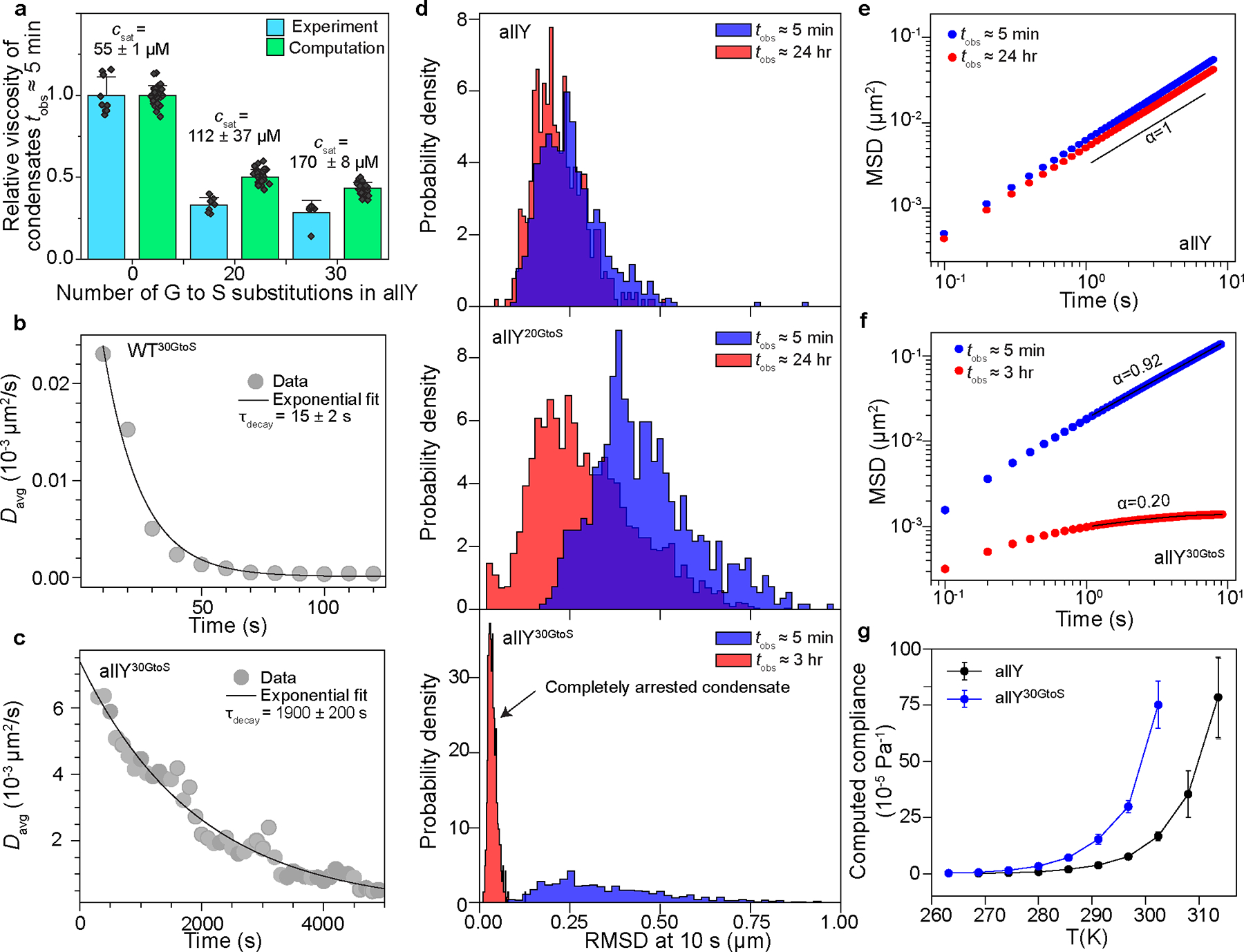
(a) Relative changes in viscosities within condensates at time of observation , calibrated against the allY system, and quantified as a function of different numbers of Gly to Ser substitutions. Data are shown for relative viscosities from measurements and computations, where the latter uses the collective model for the Zimm matrix. Error bars represent the standard deviation in the estimate of the mean relative viscosity. Experimental viscosities are obtained from at least 6 experiments ( for allY, for allY20GtoS, and for allY30GtoS) featuring at least 50 tracked particles in each measurement. Saturation concentration values shown for ≈ 20 °C. (b) Average diffusion coefficient () of 200 nm polystyrene beads within WT30GtoS condensates measured as a function of time following the start of sample imaging. The black line shows an exponential decay fit with the characteristic decay times as indicated. The time zero in the graph corresponds to time of observation, . (c) Same as (b) but for allY30GtoS condensates. (d) Histograms for the Root Mean Squared Displacement (RMSD) of 200 nm polystyrene beads measured at 10 s lag times within condensates at and . The top, middle, and bottom panels show histograms for condensates at different times of (ages of condensates are in the legends) formed by allY, allY20GtoS, allY30GtoS, respectively. (e) Ensemble-averaged Mean Squared Displacement (MSD) of 200 nm beads in allY condensates at (blue) and (red). The solid black line is the fit to the equation . The value of the exponent obtained from the fit shows diffusive motion. (f) Same as (e) but for allY30GtoS condensates. The values of the exponents show the onset of sub-diffusive motion. For panels (b)-(f), the experiments were repeated at least three times. (g) Temperature-dependent compliance computed from the simulations for condensates formed by allY and allY30GtoS. T is temperature in Kelvin (K). We use the collective model for computing the Zimm matrix. Error bars are standard deviations of the mean compliance values computed using 3 replicates. Solid lines connect the data points.
In the absence of spacer mutations, the ensemble-averaged MSDs of probe particles within allY condensates did not show any significant alterations even after 24 hrs (Fig. 3e). In contrast, the MSD measurements showed age-dependent dynamics for condensates formed by the allY20GtoS and allY30GtoS variants (Extended Data Fig. 4c, d, and Fig. 3f). After , the observed MSD curves show sub-diffusive motion of the probe particles (Fig. 3f). The translational diffusion of probe particles likely becomes caged due to the onset of stable elastic networks 20,45–47 in condensates formed by allY30GtoS (Fig. 3d, bottom).
The zero-shear compliance quantifies the maximal network reconfiguration achievable at a given stress. The compliance was found to be higher for variants with increased numbers of Gly-to-Ser substitutions (Fig. 3g). Increased compliance enables facile network rearrangements. These network rearrangements appear to engender a mismatch in timescales whereby rapid mobilities are hindered by the high density of crosslinks, thus leading to dynamical arrest 7. If this is valid, then the allY30GtoS condensates should become dominantly elastic as increases. We tested this prediction by calculating viscoelastic properties as a function of via analysis of MSDs of the probe particles (see Methods and Supplementary Fig. S2) 48,49. Upon converting the measured values of MSDs to complex moduli, we find that allY30GtoS condensates are primarily viscous at (Extended Data Fig. 5d–5f). The elastic modulus increases dramatically upon physical aging for condensates of allY30GtoS. The overall shapes of the frequency-dependent viscoelastic moduli resemble that of Kelvin-Voigt solids (Extended Data Fig. 5a–c; 5g–i) and confirm that allY30GtoS condensates are dominantly elastic at long observation times ().
Aged condensates are dominantly elastic Kelvin-Voigt solid.
To further investigate the nature of dynamical transitions that accompany condensate aging upon mutations of spacer residues, we employed active microrheology using an optical tweezer-based creep test 50 (Fig. 4a and Extended Data Fig. 6a). A polystyrene particle is trapped within the condensate and dragged through the condensate at a constant velocity (Fig. 4a). We recorded how the particle follows the traveling optical trap while simultaneously measuring forces exerted on the particle by the condensates. For a material with dominantly viscous behavior, the particle should follow the trap until it is stopped. It will remain at the new position once the trap is stopped 51 (Fig. 4b, top and Extended Data Fig. 6a, bottom). For a dominantly viscous Maxwell fluid, the bead will also follow the trap but with a lag time that is governed by the dominant relaxation time of the fluid 51 (Fig. 4b, middle and Extended Data Fig. 6a, middle). For a dominantly elastic material such as a Kelvin-Voigt viscoelastic solid, the particle will follow the trap before recoiling to its initial position 51 (Fig. 4b, bottom and Extended Data Fig. 6a, top).
Fig. 4: Dynamically arrested A1-LCD condensates are Kelvin-Voigt solids with dominantly elastic behavior.
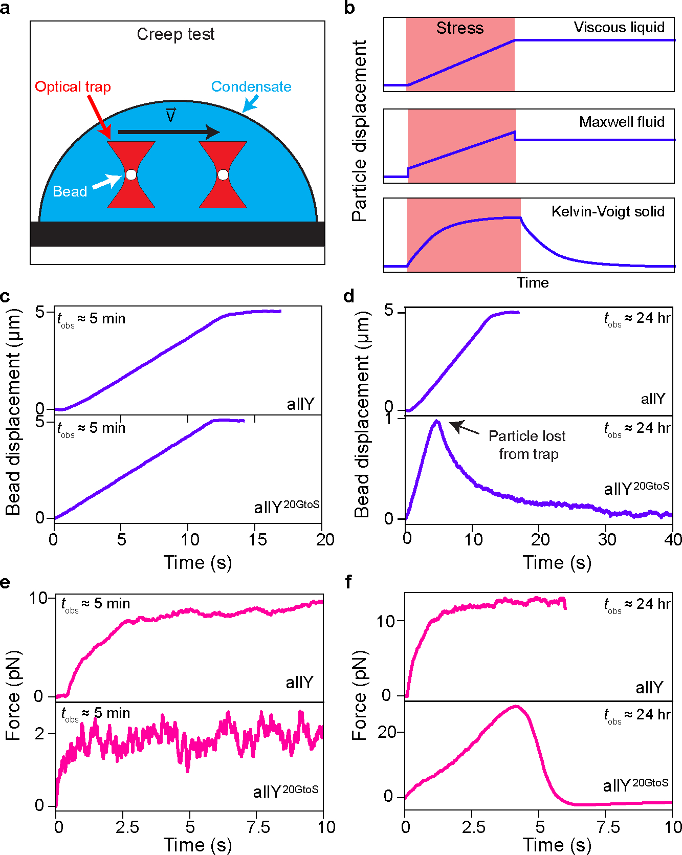
(a) Schematic of the optical tweezer-based creep test microrheology experiment. A bead (white circle) is trapped within a condensate (blue shading) using an optical trap (red hourglass shape). The trap is programmed to move a set distance (here 5 μm) at a constant velocity (0.5 μm/s). The bead position and the force exerted by the condensate on the bead are monitored via a camera and a quadrant photodetector, respectively. The black rectangle represents the slide surface. (b) Expected bead displacement in response to the trap movement during the creep test for a viscous liquid, a viscoelastic Maxwell fluid, and a Kelvin-Voigt solid. The red-shaded regions depict the period over which the stress is applied. (c) Bead displacement as a function of time in response to the programmed trap movement in allY and allY20GtoS condensates at the time of observation, . (d) Same as (c) but for aged allY and aged allY20GtoS condensates (). Note that the bead in the allY20GtoS condensate recoils back to its initial position after ~1 μm travel, indicating that the condensate is exerting an elastic force that overpowers the force exerted by the optical trap. As shown in panel (b), this response is characteristic of a viscoelastic solid. (e) Force exerted on the bead by the condensate network during the creep test experiment. Data are shown for allY and allY20GtoS condensates at . The saturation of the force is a characteristic of the viscous drag force, which depends on the velocity of the trap, the viscosity of the condensate, and the size of the bead. (f) Same as (e) but for condensates at . The data in the bottom of panel (f) indicate that aged condensates formed by allY20GtoS behave like Kelvin-Voigt solids. Comparison with the top panel highlights the fact that these condensates transition from being Maxwell fluids at early time points to dominantly elastic, Kelvin-Voigt solids as they age. The experiments were repeated at least three times.
We performed optical tweezer-based creep tests on allY and allY20GtoS condensates. At , both condensates showed dominantly viscous fluid behavior (Fig. 4c). At , the allY condensates still displayed dominantly viscous behaviors (Movie S2, Fig. 4d, top). However, the allY20GtoS condensates exhibited behaviors consistent with a Kelvin-Voigt viscoelastic solid (Movie S3, Fig. 4d, bottom). In dominantly viscous allY and allY20GtoS condensates, the saturation of the force is a characteristic of the viscous drag force 52, which depends on the velocity of the trap, and the viscosity of the condensate, but is independent of the distance (Fig. 4e, top). This behavior is preserved for the allY condensates investigated at (Fig. 4e, bottom), and is very different for the aged condensates formed by allY20GtoS (Fig. 4f, top versus bottom). We systematically increased the stiffness of the trap by increasing the trapping power and observed that the maximum displacements traversed (Extended Data Figs. 6b, 6c) and the force traces for the bead within allY condensates do not show changes over 24 hours (Extended Data Figs. 6f, 6g). In contrast, the maximum distance traveled by the particle decreased and the maximum force it experienced increased for allY20GtoS condensates over time (Extended Data Figs. 6d, 6h, 6e, 6i). This indicates that the restoring force responsible for the particle recoil in aged allY20GtoS condensates is predominantly elastic (Supplementary Note 5).
Elastic A1-LCD condensates are semi-crystalline materials.
Next, we asked if dynamical arrest induces changes to the mesoscale morphologies of condensates. Differential interference contrast (DIC) microscopy (Fig. 5a) shows that the micron-scale appearance of nascent and aged condensates formed by allY20GtoS remain essentially the same (Fig. 5a). Additionally, while the Thioflavin (ThT) dye shows positive staining for fibrils formed by a positive control, insulin, at , it does not show positive staining for any of the aged PLCD condensates studied in this work (Fig. 5b). Next, we used Fourier transform infrared (FTIR) spectroscopy to study condensates at different values of . Signals at different wave numbers in FTIR spectra can be referenced to extant basis sets to assign the contents of different types of secondary structures (Extended Data Fig. 7a). Condensates characterized at are disordered (Extended Data Figs. 7b, 7c, 7d and 7e). While the FTIR spectra change minimally for allY over a 24-hour period (Fig. 6a), the spectra for allY30GtoS show a clear change as a function of time (Fig. 6b). Specifically, we observed time-dependent increases in beta-sheet contents for allY30GtoS. This is concordant with a two-state transition 53 as evidenced by the presence of an isosbestic point (Fig. 6c). Insulin amyloid fibers show FTIR spectra that bear qualitative resemblance to the aged condensates of allY30GtoS (Fig. 6b versus Extended Data Fig. 7h). However, plotting the second derivative spectra, and contributions of different components of the basis sets show quantitative differences. The area under the peak corresponding to “aggregated beta sheets” increases with for allY30GtoS (Extended Data Figs. 7e, 7f, 7g). The beta-sheet-contents of insulin amyloid fibers (Extended Data Figs. 7h, 7i) are more than two-fold higher when compared to the condensates of allY30GtoS. The beta-sheet-contents increase with time, and this represents a disorder-to-order transition as a function of (Extended Data Fig. 7j).
Fig. 5: Aged A1-LCD condensates show identical mesoscale morphology and absence of amyloid fibrils.

(a) Representative images from no fewer than four DIC microscopy images of different condensates at time of observation and at . Insulin fibrils are shown as positive control. (b) ThT fluorescence ratios of the maximal / minimal intensities for freshly prepared condensates and condensates at for various A1-LCD variants. No changes were observed in ThT staining for condensates formed as a function of aging. As a positive control, we show data for amyloid fibrils formed by insulin after 24 hrs from sample preparation. At least four independent samples were prepared for each variant. Each diamond represents an individual data point, and the horizontal line indicates the mean.
Fig. 6: Aged A1-LCD condensates are beta-sheet-containing non-fibrillar, semi-crystalline solids.

(a) Fourier transform infrared (FTIR) spectra for allY condensates at time of observation and . (b) -dependent FTIR spectra for condensates of allY30GtoS. (c) Difference spectra referenced to , shown as change in absorbance units (ΔAU), show a decrease in signal for non-beta-sheeted regions and an increase in signal for beta-sheets, specifically aggregated beta-sheets (see Extended Data Fig. 7a). The difference spectra also reveal the presence of an isosbestic point, which is suggestive of a two-state disorder-to-order transition. (d) Freeze fracture deep-etch EM images of condensates of allY30GtoS imaged at . (e) Zoom-in image of a semi-crystalline material formed by allY30GtoS. The semi-crystalline morphology is annotated by the presence of three regions labeled I, II, and III, which refer to an amorphous core (I), a lamellar crystalline region (II), and a halo generated by the reorientation of the samples during imaging. This halo is caused by the softness of the materials. Panels (d) and (e) are representative of a single sample.
Next, we used freeze-fracture, deep-etch electron microscopy (EM) to probe the supramolecular organization of dominantly elastic condensates formed by allY30GtoS (Fig. 6d). The structures reveal a dense dark region that is consistent with an amorphous as opposed to crystalline organization (region I in Fig. 6e). However, the material is semi-crystalline, as evidenced by the lamellar ordering at the interface (region II in Fig. 6e). The materials are soft, and this causes a roll over that creates a halo as the sample is reoriented for deep etch EM imaging (region III in Fig. 6e). Overall, the picture that emerges is of beta-sheet-containing, non-fibrillar semi-crystalline materials that form as the condensates age.
Outlook
Our systematic assessments of sequence-specific and age-dependent material properties of condensates formed by A1-LCD and variants thereof reveal that these condensates are metastable viscoelastic fluids. The crossover timescale between dominantly elastic (short timescale) and dominantly viscous (long timescale) behaviors is governed by the strengths of sticker-mediated interactions. The storage and loss moduli increase by at least an order of magnitude as sticker strengths increase. Upon aging, we observe disorder-to-order transitions leading to semi-crystalline, non-fibrillar, beta-sheet-containing dominantly elastic materials that are congruent with being Kelvin-Voigt solids (Supplementary Note 5).
We propose that the condensation of A1-LCD-like systems is best described using a bistable model whereby the free energies of dense phases are written in terms of an order parameter (), which quantifies the extent of structural ordering on the manifold of fixed density () (Fig. 7). This proposal combines the Landau picture 54 of phase transitions along and the Zwanzig picture 55 of roughness within the disordered fluid phase. Dominantly viscous Maxwell fluids are metastable, disordered phases defined by low values of the order parameter . Fluid-to-solid transitions are disorder-to-order transitions and the likelihood of realizing this transition will be governed by the height of the barrier between the Maxwell fluid and Kelvin-Voigt solid (Fig. 6).
Fig. 7: Proposed free energy profile showing bistability and intra-well ruggedness.

The well corresponding to low values of the order parameter is a disordered, terminally viscous Maxwell fluid. The well on the right, corresponding to high values of the order parameter is the ordered, Kelvin-Voigt solid. The barrier for disorder-to-order transitions is expected to be high, , for condensates formed by naturally occurring PLCDs. This barrier is lowered, by destabilizing fluid-like states via mutations to spacers that increase their effective solvation volumes. Within the metastable and globally stable wells, we expect there to be ruggedness due to polymorphisms in the solid phase, and the contributions from conformational heterogeneity in the fluid phase. In a spring-dashpot representation, the spring (elastic element) is in series with the dashpot (viscous element) for a Maxwell fluid and in parallel for a Kelvin-Voigt solid. Conversion between material states can be depicted using a Zener model, which includes springs in series (E2) and in parallel (E1). The relative importance of E2 versus E1, depicted by pale versus bold coloring of the springs, is used to depict the conversion between states where E2 is dominant to states where E1 is dominant. The ruggedness we depict for the metastable fluid phase well is captured by the flow activation energy measurements. is the free energy of the condensate with fixed density , represented in terms of the order parameter .
Given the large barriers we estimate for network rearrangements (Fig. 2c, 2d), it appears that for many naturally occurring systems, including PLCDs, the barrier to conversion from metastable viscous fluids to globally stable elastic solids might be insurmountable on biologically relevant timescales, especially for those that are turned over rapidly. This might explain why “dynamicity” is often invoked as a key determinant of condensate functions in cells 16,18,19. In contrast to condensates that turn over, Balbiani bodies are long-lived condensates 56. Here, the sequence grammars appear to enable facile conversion to dominantly elastic solid phases 57.
Methods
Details of the protein construct design and purification, measurements to construct phase boundaries, glass slide and coverslip preparation, sample preparation and chamber assembly, differential interference contrast (DIC) microscopy and Thioflavin T (ThT) assay, Fourier Transform Infrared (FTIR) spectroscopy, insulin fibril preparation, deep etch electron microscopy, and calculation of the complex shear modulus from video particle tracking microrheology are provided in the Supplementary Materials and Methods.
Temperature-controlled video particle tracking (VPT)
We prepared the protein condensates in a buffer that contained 200 nm carboxylate-modified yellow-green beads (Invitrogen) as described in the sample preparation section above. The sample was allowed to equilibrate for a few minutes before loading it onto the microscope for imaging. Fluorescence imaging of the sample was performed using a Zeiss Primovert inverted microscope equipped with a 40× air objective and a Teledyne FLIR blackfly S USB3 CMOS camera. The microscope also contained a custom-designed thermal stage (INSTEC) with a heat insert to fix and measure the temperature of the sample through a thermocouple. The exposure time was set to 100 ms, which is also the frame time of the movies (the frame rate is 10 frames per second). Movies of the beads diffusing within the condensate were recorded for 2 to 5 minutes and saved for further analysis. For the room temperature viscosity measurements, all analyses were performed using at least six individual condensates through multiple sample preparations. For the condensate aging experiments, we used a 100× oil immersion objective. For the flow activation energy measurements, condensates were first equilibrated to the lowest experimental temperature for ~10 minutes. Movies of the diffusion of beads were then collected. The temperature was then increased to the next higher temperature and the sample was equilibrated at that temperature for ~10 minutes. This process was repeated until the upper-temperature limit was reached, which was checked to be significantly lower than the upper cloud point temperature of the variants. In some cases, droplets fused on the coverslip and formed a continuous condensed phase that is a few micrometers in height. In such cases, we imaged several fields of view and analyzed them individually to extract viscosity. The viscosity values were averaged and the error in the mean values was estimated as the standard deviation. For condensate samples where the crossover frequency is close to the upper limit of experimentally accessible frequencies in pMOT measurements, we performed high-speed VPT experiments. For these experiments (Extended Data Figs. 1d and 4c), the sample was prepared in an identical way to all other VPT samples and loaded on a Zeiss Axio Observer inverted microscope equipped with a 100× oil immersion objective. High-speed imaging (200–500 frames per second) was achieved using the back-illuminated Kinetix 22 sCMOS camera (Teledyne Photometrics).
Passive Microrheology with Optical Tweezers (pMOT)
All pMOT experiments, which yielded dynamical moduli across a frequency range that spans over two orders of magnitude, were conducted as described in detail by Alshareedah et al. 1 The theoretical basis of the method relies on the works of Preece et al., 2 Yao et al., 3 Tassieri et al., 4, as well as Mason and Weitz 5. pMOT experiments were conducted on a LUMICKS C-Trap microscope equipped with a 60× water immersion objective. Condensates were prepared in a buffer containing 1.0 μm beads. Condensates were allowed to settle on the surface of the coverslip for ~20 minutes. Individual beads within condensates were trapped using the optical tweezer at minimum power (<100 μW). The trapped bead was positioned at the center of the condensate in the xy plane and ~3 μm above the glass surface. The bead trajectory was tracked using a built-in tracking algorithm through the bright field camera of the microscope at a rate of 500 Hz. Bead trajectories were collected for 5 to 20 minutes and saved for further analysis.
Optical tweezer-based creep test
The laser tweezer-based creep test was performed similarly as pMOT experiments. In the creep tests, a polystyrene particle is trapped within the condensate and dragged through the condensate at a constant velocity (Fig. 4a). This ensures a constant strain rate within the condensate. Specifically, we programmed the optical tweezer to travel 5.0 μm at a speed of 0.5 μm/s. The optically trapped bead (2 μm in diameter) was imaged as it responded to the traveling trap and the bead trajectory within the field of view was tracked using the bright field camera. Simultaneously, we measured the forces exerted on the particle by the internal networks of condensates. For each system, we performed the creep test at five different trapping laser powers (1–5 % with an increment of 1%, 10–50 μW). Prior to each creep test measurement, the trajectory of a stationary bead was collected for 2 minutes at the respective tracking power. This trajectory was used for the optical trap calibration (see data analysis section). The force experienced by the bead was obtained by measuring the displacement of the bead from the center of the optical trap using a quadrant photodiode.
Graph-theoretic implementation of Rouse-Zimm theory
In both the single-chain and collective models, all rheological properties were calculated from the eigenvalues of the Zimm matrix and averaged over the ensemble. The first eigenvalue is zero 6. For the mode, each non-zero eigenvalue is inversely proportional to the relaxation time , given by 7:
| (1) |
In (1), the temperature is in simulation units with the Boltzmann constant set to unity. The Kuhn length and friction coefficient of the medium are also set to unity. To calculate the dynamical moduli, we first calculated the relaxation modulus from a linear superposition of the eigenmodes 8 as a function of time :
| (2) |
In (2), is the number of nodes (beads in the Rouse-Zimm theory). We set the weights and volume fraction to be unity. The latter choice reflects the fact the Rouse-Zimm theory was designed for polymer melts. This choice was also made to enable unbiased rescaling to put the computed moduli on the same footing as the experimental data.
The frequency-dependent complex shear modulus was calculated from the Fourier transform of equation 2 8. The computed frequency range is greater than the shortest and longest relaxation times to ensure that we capture all the relevant dynamics. The values of and at the single point corresponding to the crossover of the storage and loss moduli were rescaled by a multiplicative factor so the computed and measured crossover frequencies match one another. This represents a single-parameter-based rescaling that puts the computed and measured moduli on the same scale, thereby allowing us to quantitatively assess if the computed moduli match the measured moduli. Note that the computations only use information about the ensemble-averaged network structure within condensates. If information that is missing from the simulations ends up contributing to most of the measured moduli, then rescaling to match the crossover frequency, which uniformly shifts the computed frequency spectrum, will not lead to a matching of the computed and measured moduli. However, as shown in the main text, the simple rescaling operation is sufficient not only to bring the measured and computed moduli onto the same scale, but we also observe close correspondence across several orders of magnitudes of frequencies. We find that the agreement between computed and measured moduli is superior for the collective model, especially for computed storage moduli. This highlights the fact that storage moduli depend on the collective behavior of the condensate-spanning network. The use of the single, sequence-specific rescaling parameter is justified on the grounds that the weights in equation 2 are not known a priori. However, what we show is that we do not need to compute each of the weights separately. Instead, a single, uniform rescaling is sufficient for facilitating comparisons between experiments and computations.
Computations were carried out for all variants of A1-LCD reported in Farag et al 9, for FUS-LCD and for a homopolymer that was tuned to give rise to phase behavior closely matching that of A1-LCD WT-NLS 9 (Table S2).
Two other quantities, namely the zero-shear viscosity and the steady-state compliance, can be derived from the moments of the gyration tensor 10. Using the spectrum of relaxation times given by equation 1, we can express the zero-shear viscosity as:
| (3) |
The steady-state compliance is computed using:
| (4) |
where the volume fraction at a given temperature is computed using the volume fractions of the dense and dilute phases using: .
Data analysis
Temperature-controlled video particle tracking
Video particle tracking (VPT) measurements monitor the movement of beads inside the condensates and output movies which can be further analyzed to get the mean square displacement (MSD) of the beads 11. MSDs can be used to estimate other quantities of interest such as diffusion coefficients, diffusivity exponents, and viscosity. We first used the TrackMate plugin of ImageJ FIJI software to track the diffusion of beads and produce two-dimensional trajectories of each bead within the condensates 12. Next, we calculated the diffusion of the center of mass of beads by computing the center of mass vector at each time point. Calculation of the center of mass vector was performed using particle velocities according to the following equation:
| (5) |
Here, is the initial center of mass vector calculated by averaging the coordinates of all beads in the first frame (k=1), is the mean velocity of all particles in frame is the velocity of particle in frame in units of μm/frame and is the number of particles in frame . The quantity is the frame difference which is included in the equation to have correct units but is set to 1 since we are analyzing consecutive frames. This method of center-of-mass (COM) calculation from particle velocity is insensitive to the appearance or disappearance of particles from the field of view, which can lead to false COM shifts if calculated using the conventional definition. Once the COM is calculated, we subtract it from the individual bead trajectories to ensure the absence of any sample drift in the data. Following that, we calculate the ensemble and time averaged mean squared displacement (MSD) using:
| (6) |
In (6), is the lag time. Next, we extracted the diffusion coefficient of the beads by fitting the MSD to the following equation:
| (7) |
Here, is the diffusion coefficient, is the diffusivity exponent, and is a term to account for the tracking noise. For fluids with terminally viscous behavior, approaches 1 at long lag times which allows for the calculation of the terminal viscosity through the Stokes-Einstein equation:
| (8) |
Here, is the particle radius, is the Boltzmann coefficient, and is the temperature in Kelvin. The averaged value was reported for the viscosity from several condensates. The error was estimated as the standard deviation.
For the probability density analysis reported in Fig. 3 of the main text, we computed the time averaged MSD of individual particles at a lag time of 10 seconds.
| (9) |
The values for the root-mean square displacement () were then plotted as normalized histograms using the matplotlib python library.
For the calculation of the average diffusion coefficient, we split the long movie that we collected into shorter movies consisting of 200 frames (20 seconds) starting at different time points from the start of the experiment. For each movie, the apparent instantaneous diffusion coefficient was calculated using:
| (10) |
We used this method of estimating since fitting the time-dependent MSD with equation (7) yielded diffusivity exponent values , which results in the parameter having units that are different from a canonical diffusion coefficient. Finally, we plotted the apparent average diffusion coefficients as a function of time.
Flow activation energy analysis 11
Viscosities of A1-LCD condensates were calculated at different temperatures as per the description of the temperature-controlled VPT section. The viscosities are expected to decay exponentially with increasing temperature according to the Arrhenius law of viscosity 13:
| (11) |
In (11), is the pre-exponential entropic factor, is the flow activation energy, is the universal gas constant, and is the temperature. Taking a natural logarithm of both sides of this equation yields
| (12) |
We plotted the natural log of viscosity against and fitted the data with a linear equation . The slope of the straight line is , from which we calculated the flow activation energy 11. These experiments were repeated three times, and the average value of the activation energy was reported. The error was taken as the standard deviation.
Passive microrheology with optical tweezers and the creep test
Trajectories of trapped beads were analyzed in two steps: (a) calibration of the optical trap, and (b) computation of the complex shear modulus also referred to as the viscoelastic modulus 14. For calibration, trajectories in and were corrected for drift using a cubic spline-fitting algorithm to remove the long-time drift of the particle. Next, the variance of the positional fluctuations in the and directions was computed. The trap stiffness was then computed using the equipartition theorem 15:
| (13) |
where is the Boltzmann constant and is the temperature in Kelvin.
To calculate the complex shear modulus, we first computed the normalized position autocorrelation function . This was done via the multipletau Python library. Next, the autocorrelation function was Fourier transformed into the frequency domain 4. We next calculated the complex shear modulus using the relation:
| (14) |
In (14), is the trap stiffness in or dimension and is the trapped particle radius. After the analysis of data from all tested condensates (~20 condensates and ~40 one-dimensional trajectories), the values of and were averaged at each frequency and the error was estimated as the standard deviation. The top and bottom 5% of the data were excluded as outliers. More details on this method can be found in our earlier work 14.
For the creep test, the optical trap was calibrated using the equipartition theorem as described above by monitoring the trajectory of a bead in a stationary optical trap. Then, forces were computed by multiplying the trap stiffness by the position of the bead from the center of the optical trap, which is measured using a quadrant photodiode (LUMICKS, C-trap). The absolute bead position within the field of view was measured using a camera, which was then normalized by the bead coordinates at the start of the experiment before the trap motion was initiated. Both bead positions and forces were calculated and plotted using custom Python codes (see Software section below).
Software
pMOT and VPT analysis were done using custom-made python scripts that are available on GitHub (see https://github.com/BanerjeeLab-repertoire/Material-properties). Fiji-ImageJ (version 1.53c) was used for image processing. Origin (2023) was used for Graphing. Adobe Illustrator CC (2019, v23.0) was used for the figure assembly and production. ZEN (blue, v2.3) and micromanager v2.0 were used for image collection on Zeiss Primovert microscopes. Bluelake (v1.6.11) was used for image recording and particle tracking using a Lumicks C-Trap microscope. FTIR spectra were processed and analyzed using OriginPro 2023. All details for reproducing the graph-theoretic analysis and custom-made scripts are available on GitHub (see: https://github.com/Pappulab/Material-properties).
Extended Data
Extended Data Fig. 1. Protein network structure governs condensate viscoelasticity.

(a) Representative positional trajectory, tracked along the horizontal axis, of a bead thermally fluctuating within the optical trap inside the condensate. (b) The normalized autocorrelation function (), where is the lag time, of positional fluctuations of a bead, confined by the optical trap, inside a condensate. The correlation functions measured along the horizontal and vertical axes are shown. (c) Ensemble-averaged mean square displacement (MSD) of 200 nm beads in condensates formed by WT+NLS. The solid line is a fit to the equation and reveals that at longer timescales (>10 ms) the beads are diffusive. However, at shorter timescales (<10 ms), the beads are sub-diffusive, indicating that the condensates are dominated by an elastic response. The MSD shown in black represents the average noise floor of the measurements. (d) Residuals between computed and measured storage moduli () for WT+NLS condensates. These residuals are shown for the single-chain model (red) and collective model (magenta). The residuals were computed as the absolute values of differences between the logarithms of the computed and measured moduli. Values of zero imply exact matches, values of one imply a discrepancy of an order of magnitude, and so on. At low frequencies, the sharp increase in residuals for the collective model is due to increased noise in the experimentally derived storage moduli. (e) Residuals between computed and measured loss moduli () using the single chain (blue) or collective chain models (black). The residuals were computed as in panel (d). (f) Comparison of computed and measured dynamical moduli for WT+NLS condensates. The computations use the single-chain model with weighted Zimm matrices. The computed crossover frequency was rescaled to match the experimental value. No other adjustments or fitting of the data was performed. The inadequacy of the single-chain model is made clear by the fact that this model overestimates the storage modulus by almost two orders of magnitude. Similar overestimates were found for other systems, and they stand in contrast to the results obtained using the collective model shown in Fig. 1b. The error band for the computed data represents the standard deviation from 3 replicates. (g) Comparison of computed and measured dynamical moduli for WT+NLS condensates with computations that use the single-chain model with unweighted Zimm matrices. The computed dynamical moduli were rescaled as in panel (f). In (f)-(g), the standard deviation from 3 replicates is smaller than the line width used to plot the computed moduli. The error bars for measured data in (f)-(g) represent standard deviations about the mean (± S.D.M.) that were computed using data for 20 separate beads over 3 independent experiments. (h) A schematic diagram of the constructs deployed in the various measurements in this work is summarized. Grey represents non-aromatic spacer residues, whereas colored stripes represent the locations of the indicated aromatic residues.
Extended Data Fig. 2. Viscoelastic moduli of condensates formed by A1-LCD mutants.

(a) Computed dynamical moduli (elastic () and viscous ()), calculated using the collective model, for condensates formed by allF. The error band for the computed data represents the standard deviation from 3 replicates. (b) Measured and for condensates formed by the YtoW variant. The error bars for measured data represent standard deviations about the mean (± S.D.M.) that were computed using data for 20 separate beads over 3 independent experiments. (c, d) Measured and for condensates formed by W- and FtoW variants, respectively. The error bars for measured data in (f)-(g) represent standard deviations about the mean (± S.D.M.) that were computed using data for 20 separate beads over 3 independent experiments.
Extended Data Fig. 3. Temperature-dependent viscosities report on the flow activation energies of the condensates.

(a) Schematic for the temperature-dependent video particle tracking (VPT) measurements. The 200 nm beads (yellow circles) are embedded inside the condensate (blue region) sitting on a substrate (black rectangle). Diffusion of multiple 200 nm polystyrene beads is recorded using 100x objective (grey box) at distinct temperatures (depicted with blue and red symbols for cold and hot). (b) Room-temperature bulk dynamical viscosity of condensates formed by different sequence variants as measured by VPT compared to passive microrheology with optical tweezers (pMOT). Data for viscosities from VPT were collected from at least six trials (n=7 for allF, n=9 for allY, n=6 for WT+NLS, n=7 for W-, n=13 for YtoW, n=6 for FtoW, and n=6 for allW) featuring at least ~50 tracked particles per trial. Error bars represent standard deviations about the mean (± S.D.M.). Although the viscosity values obtained from these two independent experimental measurements are in good agreement with one another, we note that the terminal zero-shear viscosity, obtained from the slope of the frequency-dependent loss modulus in pMOT measurements, is an asymptotic property, which means that this quantity is difficult to estimate for viscoelastic materials when the elastic and viscous moduli become similar, even below the crossover frequency. The low-frequency limit of the measurement (about 0.1 Hz which corresponds to ~10 s) may not be low enough to estimate the zero-shear viscosity, especially for condensates with high viscoelasticity, such as for variants with Trp residues as stickers. This explains the minor discrepancy in the viscosity values obtained from VPT and pMOT measurements. (c) Representative plots of the ensemble-averaged mean squared displacement (MSD) of 200 nm polystyrene beads within condensates formed by allF. Measurements were performed using VPT-based microrheology at different temperatures as set by a custom-made thermal stage attached to the microscope. (d) Measured temperature-dependent viscosities for the condensates formed by different sequence variants of A1-LCD. The solid lines connect the data points but do not represent fits. Temperature-dependent viscosities were collected from at least five trials (n≥5) for each temperature, featuring at least ~50 tracked particles per trial. Error bars represent standard deviations about the mean (± S.D.M.). (e) Arrhenius plots of measured viscosities for condensates formed by allW, WT+NLS, allY, and allF. (f) Arrhenius plots using temperature-dependent viscosities from simulations analyzed using the collective model. Data are shown for condensates of allF, WT+NLS, and allY. (g) Flow activation energies are estimated from computations. These energies are shown in units of RT, where temperature, T = 25 °C, and R is the ideal gas constant in units of kcal / mol-K. The variant names were taken from the work of Bremer et al., (ref. 32) and Farag et al., (ref. 8). The diamonds represent the activation energy, and the whiskers represent the standard deviation in the flow activation energy calculated from the fit, pink diamonds are the hnRNP A1 variants, black diamonds highlight the homopolymer and FUS-LCD values.
Extended Data Fig. 4. Interplay between sticker strength and spacer solvation determines the timescale of the dynamical arrest of A1-LCD condensates.

(a) Schematic denoting the position of glycine to serine substitution in the WT+NLS and allY sequence backgrounds. Grey shading represents unmutated or tyrosine residues that were not mutated to serine (b) Trajectories of a 200 nm bead within condensates of WT30GtoS. Two different trajectories are shown, one at the time of observation (blue), and the other for (red). These data show that WT30GtoS condensates undergo rapid dynamical arrest within a short time. (c) Ensemble-averaged mean square displacements (MSD) of 200 nm beads diffusing within allY20GtoS condensates tracked at a high acquisition rate of 500 fps. The solid blue line is a fit to the equation . Also plotted is the average noise floor (black). These data show that allY20GtoS condensates are viscoelastic Maxwell fluids at small , with a terminal behavior of a viscous fluid (α = 1). (d) Ensemble-averaged MSD of 200 nm beads (tracked at an acquisition rate of 10 fps) in condensates formed by allY20GtoS. The MSDs were measured at different values of . Solid lines are the fits to the equation . Also indicated are the values of the exponents obtained from the fits, which show a clear deviation from the linear behavior for the aged condensates, and the onset of sub-diffusive motions.
Extended Data Fig. 5. A1-LCD condensates undergo an age-dependent transition from Maxwell fluid to Kelvin-Voigt solid.

Schematic representation of the linear viscoelastic response of (a) an elastic solid, (b) a viscous liquid, and (c) a Kelvin-Voigt viscoelastic solid. (d-f) Storage () and loss () moduli of allY30GtoS condensates at the time of observation as calculated from the measured mean squared displacements (MSDs) of embedded 200 nm probe particles (Fig. 3f in the main text). The calculations were performed following the Evans method (d) and the Mason method (e, see Supplementary Methods). A comparison between the results obtained from the two methods is shown in (f). (g-i) Same as (d-f) but for allY30GtoS condensates at .
Extended Data Fig. 6. Dynamically arrested A1-LCD condensates are dominantly elastic.

(a) Schematic showing the expected outcomes of a particle embedded within a viscoelastic Kelvin-Voigt solid (top), viscoelastic Maxwell fluid (middle), and viscous liquid (bottom) upon creep deformation by an optical trap. and represent the spring constants for the condensate and the trap, respectively, and is the viscosity of the condensate. As the optical trap exerts a force to drag a particle embedded within the material, the dashpot element applies a dissipative drag force while the spring element applies a restoring force. Except for the viscoelastic solid, the creep deformation is irreversible (the final bead position is distinct from the initial bead position X0 indicated by the red vertical line). In the case of a viscoelastic solid, the bead recoils back to its initial position due to the stored energy within the elastic element. In both viscoelastic fluids and viscous liquids, the deformation energy is eventually dissipated through the dashpot or the viscous element, giving rise to a terminally viscous behavior. (b) Bead position, with respect to the initial position, as a function of time in response to the programmed trap movement in allY condensates at the time of observation at increasing power levels of the trapping laser. (c) Same as (b) but for the allY condensates at . (d) Bead position, with respect to the initial position, as a function of time in response to the programmed trap movement in allY20GtoS condensates at increasing power levels of the trapping laser. (e) Same as (d) but for the allY20GtoS condensates at . (f) The force exerted on the bead by the allY condensate network in (b). (g) The force exerted on the bead by the allY condensate network in (c). (h) The force exerted on the bead by the allY20GtoS condensate network in (d). (i) The force exerted on the bead by the allY20GtoS condensate network in (e). The percentage values in (b-i) refer to the absolute laser powers used for each measurement.
Extended Data Fig. 7. Disorder-to-order transitions accompany the dynamical arrest of A-LCD condensates.
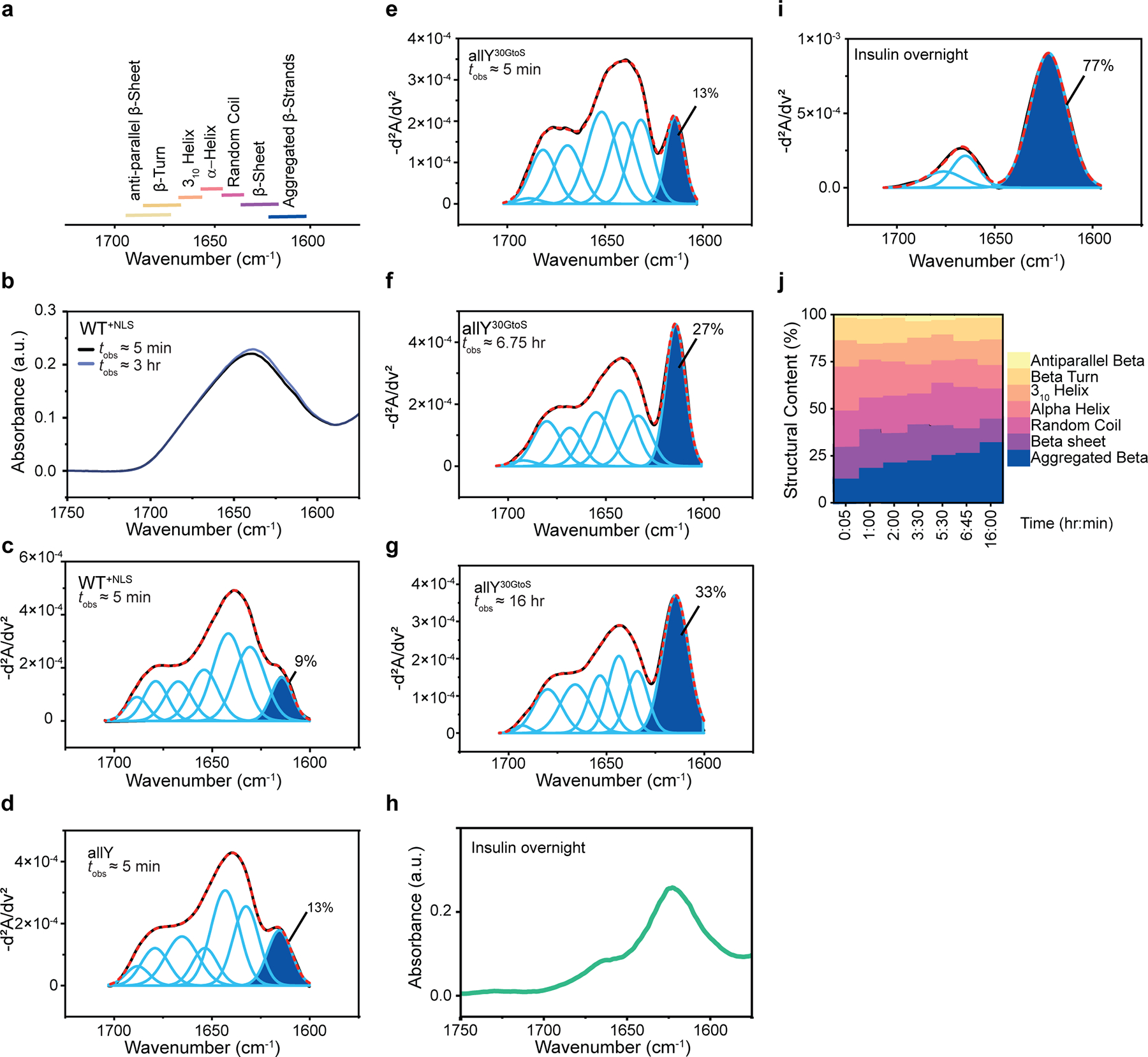
(a) Peaks in FTIR spectra correspond to the presence of specific types of secondary structures. (b) FTIR spectra for condensates formed by WT+NLS. The spectra are shown for time of observation and . (c-g and i) Inverse second derivatives (-d2A/dv2) (black line) of the measured FTIR spectra and contributions from different members of the basis set seen in (a) (light blue lines). A = absorbance; v = wave number. The dashed red line is the sum of these underlying contributions. The dark blue shading quantifies the area under the peak that corresponds to aggregated beta sheets and the estimated contribution is indicated in %. (c) Data are shown here for WT+NLS condensates for . (d) The inverse second derivative of FTIR spectra and contributions from different members of the basis set to data obtained for allY condensates at . (e) – (g) Second derivative of FTIR spectra obtained at different values of for condensates formed by allY30GtoS. (h) FTIR spectra for amyloid fibers of insulin collected at . (i) Second derivative of the measured FTIR spectra for insulin fibers and contributions from different members of the basis set. (j) Stacked plots of secondary structure contents for allY30GtoS condensates plotted as a function of time, where the abscissa refers to different values of .
Supplementary Material
Acknowledgments
This work was supported by the US National Institutes of Health through grants R01NS121114 (T.M. and R.V.P), R35 GM138186 (P.R.B), and the St. Jude Children’s Research Collaborative on the Biology and Biophysics of RNP Granules (P.R.B., T.M., and R.V.P). S.R.C. acknowledges support from the National Institutes of Health (T32 EB028092). We thank George Campbell from the Cell and Tissue Imaging Center at SJCRH, which is supported by SJCRH and NCI (grant P30 CA021765) for assistance with the DIC and confocal microscopy. We acknowledge the Washington University Center for Cellular Imaging (WUCCI), which is supported by the Washington University School of Medicine, The Children’s Discovery Institute of University and St. Louis Children’s Hospital (CDI-CORE-2015-505 and CDI-CORE-2019-813) and the Foundation for Barnes-Jewish Hospital (3770 and 4642).
Footnotes
Competing interests
RVP is a member of the scientific advisory board and shareholder in Dewpoint Therapeutics. These affiliations did not influence the work reported here. PRB is a member of the Biophysics Reviews (AIP Publishing) editorial board. This affiliation did not influence the work reported here. All other authors have no conflicts to report.
Code availability
Codes for microrheology data analysis are available on GitHub (see https://github.com/BanerjeeLab-repertoire/Material-properties). All simulation results and the code for the computation of moduli are available via the Pappu Lab GitHub (see https://github.com/Pappulab/material_properties).
Data availability
All data are available in the manuscript or the supplementary materials. All expression plasmids are available from Addgene.
References
- 1.Banani SF, Lee HO, Hyman AA & Rosen MK Biomolecular condensates: organizers of cellular biochemistry. Nature Reviews in Molecular and Cell Biology 18, 285–298, doi: 10.1038/nrm.2017.7 (2017). [DOI] [PMC free article] [PubMed] [Google Scholar]
- 2.Berry J, Brangwynne CP & Haataja M Physical principles of intracellular organization via active and passive phase transitions. Reports on Progress in Physics 81, 046601, doi: 10.1088/1361-6633/aaa61e (2018). [DOI] [PubMed] [Google Scholar]
- 3.Brangwynne CP et al. Germline P granules are liquid droplets that localize by controlled dissolution/condensation. Science 324, 1729–1732, doi: 10.1126/science.1172046 (2009). [DOI] [PubMed] [Google Scholar]
- 4.Pappu RV, Cohen SR, Dar F, Farag M & Kar M Phase Transitions of Associative Biomacromolecules. Chemical Reviews 123, 8945–8987, doi: 10.1021/acs.chemrev.2c00814 (2023). [DOI] [PMC free article] [PubMed] [Google Scholar]
- 5.Choi J-M, Dar F & Pappu RV LASSI: A lattice model for simulating phase transitions of multivalent proteins. PLOS Computational Biology 15, e1007028, doi: 10.1371/journal.pcbi.1007028 (2019). [DOI] [PMC free article] [PubMed] [Google Scholar]
- 6.Choi J-M, Holehouse AS & Pappu RV Physical principles underlying the complex biology of intracellular phase transitions. Annual Review of Biophysics 49, 107–133 (2020). [DOI] [PMC free article] [PubMed] [Google Scholar]
- 7.Ranganathan S & Shakhnovich EI Dynamic metastable long-living droplets formed by sticker-spacer proteins. eLife 9, e56159, doi: 10.7554/eLife.56159 (2020). [DOI] [PMC free article] [PubMed] [Google Scholar]
- 8.Farag M et al. Condensates formed by prion-like low-complexity domains have small-world network structures and interfaces defined by expanded conformations. Nature Communications 13, 7722 (2022). [DOI] [PMC free article] [PubMed] [Google Scholar]
- 9.Farag M, Borcherds WM, Bremer A, Mittag T & Pappu RV Phase separation of protein mixtures is driven by the interplay of homotypic and heterotypic interactions. Nature Communications 14, 5527, doi: 10.1101/2023.03.15.532828 (2023). [DOI] [PMC free article] [PubMed] [Google Scholar]
- 10.Alshareedah I, Moosa MM, Pham M, Potoyan DA & Banerjee PR Programmable viscoelasticity in protein-RNA condensates with disordered sticker-spacer polypeptides. Nature Communications 12, 6620, doi: 10.1038/s41467-021-26733-7 (2021). [DOI] [PMC free article] [PubMed] [Google Scholar]
- 11.Kota D & Zhou H-X Macromolecular Regulation of the Material Properties of Biomolecular Condensates. The Journal of Physical Chemistry Letters 13, 5285–5290, doi: 10.1021/acs.jpclett.2c00824 (2022). [DOI] [PMC free article] [PubMed] [Google Scholar]
- 12.Jawerth L et al. Protein condensates as aging Maxwell fluids. Science 370, 1317–1323 (2020). [DOI] [PubMed] [Google Scholar]
- 13.Feric M et al. Coexisting Liquid Phases Underlie Nucleolar Subcompartments. Cell 165, 1686–1697, doi: 10.1016/j.cell.2016.04.047 (2016). [DOI] [PMC free article] [PubMed] [Google Scholar]
- 14.Bergeron-Sandoval LP et al. Endocytic proteins with prion-like domains form viscoelastic condensates that enable membrane remodeling. Proc Natl Acad Sci U S A 118, e2113789118, doi: 10.1073/pnas.2113789118 (2021). [DOI] [PMC free article] [PubMed] [Google Scholar]
- 15.Wróbel JK, Cortez R & Fauci L Modeling viscoelastic networks in Stokes flow. Physics of Fluids 26, 113102, doi: 10.1063/1.4900941 (2014). [DOI] [Google Scholar]
- 16.Alberti S & Hyman AA Biomolecular condensates at the nexus of cellular stress, protein aggregation disease and ageing. Nature Reviews Molecular Cell Biology 22, 196–213, doi: 10.1038/s41580-020-00326-6 (2021). [DOI] [PubMed] [Google Scholar]
- 17.Putnam A, Cassani M, Smith J & Seydoux G A gel phase promotes condensation of liquid P granules in Caenorhabditis elegans embryos. Nature Structural & Molecular Biology 26, 220–226, doi: 10.1038/s41594-019-0193-2 (2019). [DOI] [PMC free article] [PubMed] [Google Scholar]
- 18.Li W et al. Biophysical properties of AKAP95 protein condensates regulate splicing and tumorigenesis. Nature cell biology 22, 960–972 (2020). [DOI] [PMC free article] [PubMed] [Google Scholar]
- 19.Shi B et al. UTX condensation underlies its tumour-suppressive activity. Nature 597, 726–731, doi: 10.1038/s41586-021-03903-7 (2021). [DOI] [PMC free article] [PubMed] [Google Scholar]
- 20.Shen Y et al. The liquid-to-solid transition of FUS is promoted by the condensate surface. Proc Natl Acad Sci U S A 120, e2301366120, doi: 10.1073/pnas.2301366120 (2023). [DOI] [PMC free article] [PubMed] [Google Scholar]
- 21.Wang J et al. A Molecular Grammar Governing the Driving Forces for Phase Separation of Prion-like RNA Binding Proteins. Cell 174, 688–699.e616, doi: 10.1016/j.cell.2018.06.006 (2018). [DOI] [PMC free article] [PubMed] [Google Scholar]
- 22.Boeynaems S et al. Spontaneous driving forces give rise to protein−RNA condensates with coexisting phases and complex material properties. Proc Natl Acad Sci U S A 116, 7889–7898, doi: 10.1073/pnas.1821038116 (2019). [DOI] [PMC free article] [PubMed] [Google Scholar]
- 23.Lin AZ et al. Dynamical control enables the formation of demixed biomolecular condensates. Nature Communications 14, 7678, doi: 10.1038/s41467-023-43489-4 (2023). [DOI] [PMC free article] [PubMed] [Google Scholar]
- 24.Sciortino F, Bansil R, Stanley HE & Alstrom P Interference of Phase-Separation and Gelation - a Zeroth-Order Kinetic-Model. Phys Rev E 47, 4615–4618, doi:DOI 10.1103/PhysRevE.47.4615 (1993). [DOI] [PubMed] [Google Scholar]
- 25.Zaccarelli E, Lu PJ, Ciulla F, Weitz DA & Sciortino F Gelation as arrested phase separation in short-ranged attractive colloid-polymer mixtures. J Phys-Condens Mat 20, 494242, doi:Artn 494242 10.1088/0953-8984/20/49/494242 (2008). [DOI] [Google Scholar]
- 26.Lu S et al. Heat-shock chaperone HSPB1 regulates cytoplasmic TDP-43 phase separation and liquid-to-gel transition. Nature Cell Biology 24, 1378–1393, doi: 10.1038/s41556-022-00988-8 (2022). [DOI] [PMC free article] [PubMed] [Google Scholar]
- 27.Wadsworth GM et al. RNAs undergo phase transitions with lower critical solution temperatures. Nature Chemistry 15, 1693–1704, doi: 10.1038/s41557-023-01353-4 (2023). [DOI] [PMC free article] [PubMed] [Google Scholar]
- 28.Patel A et al. A liquid-to-solid phase transition of the ALS protein FUS accelerated by disease mutation. Cell 162, 1066–1077 (2015). [DOI] [PubMed] [Google Scholar]
- 29.Molliex A et al. Phase separation by low complexity domains promotes stress granule assembly and drives pathological fibrillization. Cell 163, 123–133 (2015). [DOI] [PMC free article] [PubMed] [Google Scholar]
- 30.Mathieu C, Pappu RV & Taylor JP Beyond aggregation: Pathological phase transitions in neurodegenerative disease. Science 370, 56–60, doi:doi: 10.1126/science.abb8032 (2020). [DOI] [PMC free article] [PubMed] [Google Scholar]
- 31.Martin EW et al. Valence and patterning of aromatic residues determine the phase behavior of prion-like domains. Science 367, 694–699 (2020). [DOI] [PMC free article] [PubMed] [Google Scholar]
- 32.Bremer A et al. Deciphering how naturally occurring sequence features impact the phase behaviours of disordered prion-like domains. Nature Chemistry 14, 196–207, doi: 10.1038/s41557-021-00840-w (2022). [DOI] [PMC free article] [PubMed] [Google Scholar]
- 33.Ghosh A, Kota D & Zhou H-X Shear relaxation governs fusion dynamics of biomolecular condensates. Nature Communications 12, 5995, doi: 10.1038/s41467-021-26274-z (2021). [DOI] [PMC free article] [PubMed] [Google Scholar]
- 34.Michieletto D & Marenda M Rheology and Viscoelasticity of Proteins and Nucleic Acids Condensates. JACS Au 2, 1506–1521, doi: 10.1021/jacsau.2c00055 (2022). [DOI] [PMC free article] [PubMed] [Google Scholar]
- 35.Eichinger BE Configuration Statistics of Gaussian Molecules. Macromolecules 13, 1–11, doi: 10.1021/ma60073a001 (1980). [DOI] [Google Scholar]
- 36.Yang Y & Yu T Graph theory of viscoelasticities for polymers with starshaped, multiple-ring and cyclic multiple-ring molecules. Die Makromolekulare Chemie 186, 609–631, doi:doi: 10.1002/macp.1985.021860315 (1985). [DOI] [Google Scholar]
- 37.Rouse PE A Theory of the Linear Viscoelastic Properties of Dilute Solutions of Coiling Polymers. The Journal of Chemical Physics 21, 1272–1280, doi: 10.1063/1.1699180 (1953). [DOI] [Google Scholar]
- 38.Zimm BH Dynamics of Polymer Molecules in Dilute Solution: Viscoelasticity, Flow Birefringence and Dielectric Loss. The Journal of Chemical Physics 24, 269–278, doi: 10.1063/1.1742462 (1956). [DOI] [Google Scholar]
- 39.Peticolas WL Introduction to the Molecular Viscoelastic Theory of Polymers and Its Applications. Rubber Chemistry and Technology 36, 1422–1458, doi: 10.5254/1.3539650 (1963). [DOI] [Google Scholar]
- 40.Tesei G, Schulze TK, Crehuet R & Lindorff-Larsen K Accurate model of liquid-liquid phase behavior of intrinsically disordered proteins from optimization of single-chain properties. Proc Natl Acad Sci U S A 118 (44):e2111696118, doi: 10.1073/pnas.2111696118 (2021). [DOI] [PMC free article] [PubMed] [Google Scholar]
- 41.Joseph JA et al. Physics-driven coarse-grained model for biomolecular phase separation with near-quantitative accuracy. Nature Computational Science 1, 732–743, doi: 10.1038/s43588-021-00155-3 (2021). [DOI] [PMC free article] [PubMed] [Google Scholar]
- 42.Schlenoff JB & Akkaoui K Dissecting dynamics near the glass transition using polyelectrolyte complexes. Macromolecules 54, 3413–3422 (2021). [Google Scholar]
- 43.Alshareedah I et al. Determinants of Viscoelasticity and Flow Activation Energy in Biomolecular Condensates. Science Advances 10, eadi6539, doi: 10.1126/sciadv.adi6539 (2024). [DOI] [PMC free article] [PubMed] [Google Scholar]
- 44.Messaâdi A et al. A New Equation Relating the Viscosity Arrhenius Temperature and the Activation Energy for Some Newtonian Classical Solvents. Journal of Chemistry 2015, 163262, doi: 10.1155/2015/163262 (2015). [DOI] [Google Scholar]
- 45.Steigmann DJ & Pipkin AC Equilibrium of elastic nets. Philosophical Transactions of the Royal Society of London. Series A: Physical and Engineering Sciences 335, 419–454, doi:doi: 10.1098/rsta.1991.0056 (1991). [DOI] [Google Scholar]
- 46.Mason TG & Weitz DA Optical measurements of frequency-dependent linear viscoelastic moduli of complex fluids. Phys Rev Lett 74, 1250 (1995). [DOI] [PubMed] [Google Scholar]
- 47.Weeks ER & Weitz DA Subdiffusion and the cage effect studied near the colloidal glass transition. Chemical Physics 284, 361–367, doi: 10.1016/S0301-0104(02)00667-5 (2002). [DOI] [Google Scholar]
- 48.Evans RML, Tassieri M, Auhl D & Waigh TA Direct conversion of rheological compliance measurements into storage and loss moduli. Phys Rev E 80, 012501, doi: 10.1103/PhysRevE.80.012501 (2009). [DOI] [PubMed] [Google Scholar]
- 49.Mason TG, Ganesan K, van Zanten JH, Wirtz D & Kuo SC Particle Tracking Microrheology of Complex Fluids. Physical Review Letters 79, 3282–3285, doi: 10.1103/PhysRevLett.79.3282 (1997). [DOI] [Google Scholar]
- 50.Robertson-Anderson RM Optical Tweezers Microrheology: From the Basics to Advanced Techniques and Applications. ACS Macro Letters 7, 968–975, doi: 10.1021/acsmacrolett.8b00498 (2018). [DOI] [PMC free article] [PubMed] [Google Scholar]
- 51.Roeder RK in Characterization of Biomaterials (eds Bandyopadhyay Amit& Bose Susmita) Ch. 3, 49–104 (Academic Press, 2013). [Google Scholar]
- 52.Hu J et al. Size- and speed-dependent mechanical behavior in living mammalian cytoplasm. Proc Natl Acad Sci U S A 114, 9529–9534, doi:doi: 10.1073/pnas.1702488114 (2017). [DOI] [PMC free article] [PubMed] [Google Scholar]
- 53.Ranganathan S & Shakhnovich E The physics of liquid-to-solid transitions in multi-domain protein condensates. Biophysical Journal 121, 2751–2766, doi: 10.1016/j.bpj.2022.06.013 (2022). [DOI] [PMC free article] [PubMed] [Google Scholar]
- 54.Landau L The Theory of Phase Transitions. Nature 138, 840–841, doi: 10.1038/138840a0 (1936). [DOI] [Google Scholar]
- 55.Zwanzig R Diffusion in a rough potential. Proc Natl Acad Sci U S A 85, 2029–2030, doi:doi: 10.1073/pnas.85.7.2029 (1988). [DOI] [PMC free article] [PubMed] [Google Scholar]
- 56.Boke E et al. Amyloid-like Self-Assembly of a Cellular Compartment. Cell 166, 637–650, doi: 10.1016/j.cell.2016.06.051 (2016). [DOI] [PMC free article] [PubMed] [Google Scholar]
- 57.Holehouse AS, Ginell GM, Griffith D & Böke E Clustering of Aromatic Residues in Prion-like Domains Can Tune the Formation, State, and Organization of Biomolecular Condensates. Biochemistry 60, 3566–3581, doi: 10.1021/acs.biochem.1c00465 (2021). [DOI] [PMC free article] [PubMed] [Google Scholar]
Methods-only References
- 1.Alshareedah I, Moosa MM, Pham M, Potoyan DA & Banerjee PR Programmable viscoelasticity in protein-RNA condensates with disordered sticker-spacer polypeptides. Nature communications 12, 1–14 (2021). [DOI] [PMC free article] [PubMed] [Google Scholar]
- 2.Preece D et al. Optical tweezers: wideband microrheology. Journal of Optics 13, 044022, doi: 10.1088/2040-8978/13/4/044022 (2011). [DOI] [Google Scholar]
- 3.Yao A, Tassieri M, Padgett M & Cooper J Microrheology with optical tweezers. Lab on a Chip 9, 2568–2575, doi: 10.1039/B907992K (2009). [DOI] [PubMed] [Google Scholar]
- 4.Tassieri M, Evans RML, Warren RL, Bailey NJ & Cooper JM Microrheology with optical tweezers: data analysis. New Journal of Physics 14, 115032, doi: 10.1088/1367-2630/14/11/115032 (2012). [DOI] [Google Scholar]
- 5.Mason TG & Weitz DA Optical measurements of frequency-dependent linear viscoelastic moduli of complex fluids. Phys Rev Lett 74, 1250 (1995). [DOI] [PubMed] [Google Scholar]
- 6.Eichinger BE Configuration Statistics of Gaussian Molecules. Macromolecules 13, 1–11, doi: 10.1021/ma60073a001 (1980). [DOI] [Google Scholar]
- 7.Zimm BH Dynamics of Polymer Molecules in Dilute Solution: Viscoelasticity, Flow Birefringence and Dielectric Loss. The Journal of Chemical Physics 24, 269–278, doi: 10.1063/1.1742462 (1956). [DOI] [Google Scholar]
- 8.Rubinstein M & Colby RH Polymer Physics. (Oxford University Press, 2003). [Google Scholar]
- 9.Farag M et al. Condensates formed by prion-like low-complexity domains have small-world network structures and interfaces defined by expanded conformations. Nature Communications 13, 7722 (2022). [DOI] [PMC free article] [PubMed] [Google Scholar]
- 10.Yang Y & Yu T Graph theory of viscoelasticities for polymers with starshaped, multiple-ring and cyclic multiple-ring molecules. Die Makromolekulare Chemie 186, 609–631, doi:doi: 10.1002/macp.1985.021860315 (1985). [DOI] [Google Scholar]
- 11.Alshareedah I et al. Determinants of Viscoelasticity and Flow Activation Energy in Biomolecular Condensates. Science Advances 10, eadi6539, doi: 10.1126/sciadv.adi6539 (2024). [DOI] [PMC free article] [PubMed] [Google Scholar]
- 12.Tinevez J-Y et al. TrackMate: An open and extensible platform for single-particle tracking. Methods 115, 80–90, doi: 10.1016/j.ymeth.2016.09.016 (2017). [DOI] [PubMed] [Google Scholar]
- 13.Messaâdi A et al. A New Equation Relating the Viscosity Arrhenius Temperature and the Activation Energy for Some Newtonian Classical Solvents. Journal of Chemistry 2015, 163262, doi: 10.1155/2015/163262 (2015). [DOI] [Google Scholar]
- 14.Alshareedah I, Moosa MM, Pham M, Potoyan DA & Banerjee PR Programmable viscoelasticity in protein-RNA condensates with disordered sticker-spacer polypeptides. Nature Communications 12, 6620, doi: 10.1038/s41467-021-26733-7 (2021). [DOI] [PMC free article] [PubMed] [Google Scholar]
- 15.Neuman KC & Block SM Optical trapping. Review of Scientific Instruments 75, 2787–2809, doi: 10.1063/1.1785844 (2004). [DOI] [PMC free article] [PubMed] [Google Scholar]
Associated Data
This section collects any data citations, data availability statements, or supplementary materials included in this article.
Supplementary Materials
Data Availability Statement
All data are available in the manuscript or the supplementary materials. All expression plasmids are available from Addgene.