A Method for Treating Significant Conformational Changes in Alchemical Free Energy Simulations of Protein-Ligand Binding

Abstract

Relative binding free energy (RBFE) simulation is a rigorous approach to the calculation of quantitatively accurate binding free energy values for protein-ligand binding, in which a reference binder is gradually converted to a target binder through alchemical transformation during the simulation. The success of such simulations relies on being able to accurately sample the correct conformational phase space for each alchemical state, however this becomes a challenge when a significant conformation change occurs between the reference and target binder-receptor complexes. Increasing the simulation time and using enhanced sampling methods can be helpful, but effects can be limited especially when the free energy barrier between conformations is high or when the correct target complex conformation is difficult to find and maintain. Current RBFE protocols seed the reference complex structure into every alchemical window of the simulation. In our study we describe an improved protocol in which the reference structure is seeded into the first half of the alchemical windows, and the target structure is seeded into the second half of the alchemical windows. By applying information about the relevant correct end point conformations to different simulation windows from the beginning, the need for large barrier crossings or simulation prediction of the correct structures during an alchemical simulation is in many cases obviated. In the diverse cases we examine below, the simulations yielded free energy predictions that are satisfactory as compared to experiment, and superior to running the simulations utilizing the conventional protocol. The method is straightforward to implement for publicly available FEP workflows.

Graphical Abstract

Introduction

Accurate calculation of the binding free energy of a drug molecule to its target is one of the ultimate goals of computer-aided drug design (CADD). Of the many methods that have been deployed for this purpose,^1–4 explicit solvent based free energy simulations are the most rigorous and are so far the only method capable of reliably achieving quantitative accuracy compared to experiment. The most common algorithms used for free energy simulation include relative binding free energy perturbation (FEP), thermodynamic integration (TI) and lambda dynamics,⁵ all which currently require that the conformation of the protein-ligand complex in the initial and final states are sufficiently similar, in order to obtain accurate results. The main reason for this requirement in practical computations, when it is not explicitly required in theory, is that when the simulation starts in the initial state and the conformation difference with the final state is significant, it can be very difficult to find and converge on the correct final state. Such difficulty can in principle be overcome by arbitrarily extending the length of the simulations; however, if the barrier between the initial and final states is large compared to the ambient temperature, the computational expense will grow exponentially if such a strategy is adopted. Enhanced sampling methods have been used in FEP simulations to reduce the computational cost,^{6, 7} but have generally been limited to systems that do not display a substantial receptor conformation change. Other studies exist that successfully overcame a receptor conformation change using replica exchange molecular dynamics (REMD), but were limited to changes involving only one residue.^8–10

Often, however, the correct final state or conformation is known from experiment or can be independently predicted via many approaches other than ordinary molecular dynamics simulation, e.g. conformational search algorithms, steered molecular dynamics, etc. We demonstrate in this work that one can make significant progress in computing free energy differences in this case, by supplying as an input to the simulation the correct conformation of both the initial and final states. Alchemical relative binding free energy perturbation (FEP) is the simulation methodology we utilize in this work, although the idea of supplying correct, known end point conformers will work for other free energy simulation methods, such as thermodynamic integration (TI), as well.

Consider a hypothetical fully equilibrated FEP simulation in which we are alchemically transforming one binding ligand (lig0) to another (lig1) through many intermediate windows, and which involves large conformation changes between the receptor and/or ligands of the two native states A and B for lig0 and lig1, respectively. The equilibrium structure near the midpoint of the alchemical transformation can be complicated (and in principle different from both the initial and final state), but in the great majority of cases one certainly expects the equilibrium structure to have resemblance to structure A for most windows in the first half of the simulation, and a resemblance to structure B in the second half of the simulation.

In typical currently used protocols, an FEP simulation would start with all windows identically in either state A or state B. Some approaches apply a molecular dynamics simulation (e.g. on the order of 10s of nanoseconds) for relaxation before starting to collect energies.¹¹ However, when state B is very different from state A, it is very unlikely that such a short MD simulation would successfully relax A into B, even in the later windows when the Hamiltonian becomes predominantly or entirely B, and vice versa if starting from B. In the present paper, we investigate a simple alternative: start the first half of the windows in state A, and the second half in state B. After all, even if the simulation eventually did find the correct state of B from A, energies should not be collected during this relaxation process, as such energies would only introduce extra noise and error. This strategy of seeding different lambda windows with different initial conformations has not to the best of our knowledge been systematically explored in previous work. There is one example in literature by Wang et. al. where different pyridine ring conformations of the ligand were seeded into the first and last 50% of FEP windows.¹² However, the purpose of doing so was to illustrate that their newly implemented replica exchange with solute tempering (REST2)/FEP method could provide interconversion of conformers, and accurate binding free energy results matching experiment, regardless of where the simulation started, and not to demonstrate that having the correct starting states is in itself sufficient. In their discussion they did briefly suggest that by using known end states, REST2/FEP accuracy should be expected to improve, but no demonstration of this hypothesis has been reported subsequently.

In our study, we shall refer to the general proposal of seeding different lambda windows of the FEP simulation with different receptor-ligand conformers as multiconformational FEP (MCFEP). The specific proposed algorithm, in which half of the windows are seeded with the equilibrium conformation of receptor-ligand complex A, and half with that of receptor-ligand complex B, we shall call “half and half MCFEP” (HH MCFEP).

To allow the proposed protocol to run properly, details of the technical implementation need to be taken care of. For example, for MCFEP to work in conjunction with the well-established lambda exchange FEP simulation protocol, it is necessary that the replicas in each window have the same composition of matter, including the same number of water molecules. If the conformations associated with states A and B are derived from different experimental sources (e.g. different crystal structures), that may not be the case. It would also be tricky to solvate two solute conformers with identical number of water molecules for differences larger than the one example reported involving a ligand ring flip. Therefore, we have developed a generalized algorithm that starts with the conformation A structure and morphs that into alternative structures (e.g. the B conformation) as needed by carrying out simulations starting from the A state in which restraints to the B conformation solute structure are imposed. This methodology and other details are discussed below in the Methods section.

Assuming an effective technical implementation, the fundamental question is how the specific approximation we propose above - seeding the first half of the windows with conformation A, and the second half with conformation B - will perform for interesting binding affinity calculation problems. We examine a variety of systems below and in all cases tested, the “half and half” (HH) protocol does very well, generally yielding results that interpolate effectively between the results of using conformation A to start all windows, and the results of using conformation B to start all windows, and thus yielding good agreement with experiment or with accurate but much more expensive theory.

In what follows, we consider four different systems of increasing size and complexity. Three systems have known crystal structures which can be used for both the initial and final states in the FEP transformation, while one system utilizes a simulation-predicted structure not known from experiment for the final state. In all cases, when corrected for other errors such as those attributable to the force field, the half and half protocol yields a result within the normal error range of FEP calculations (~1.1 kcal/mol RMS error¹³), giving an overall root mean square error (RMSE) of 0.62 kcal/mol. By comparison, the standard FEP runs with enhanced sampling on known conformation change residues give an RMSE of 1.61 kcal/mol. We analyze the results in detail and discuss the implications for future applications.

Results

In what follows, we discuss four receptor systems in which conformational change upon ligand binding has been identified in previous work as an important determinant of the difference in binding free energy to the receptor between these ligands. The results are presented in order of increasing complexity of the conformation change. The first system, T4 lysozyme, manifests an extremely simple conformation change (predominately of a single side chain rotamer state), which serves as an illustrative, physically transparent example of the behavior of the HH methodology as compared to conventional FEP simulations starting from either endpoint. The Hsp90 system involves a much more complicated (but localized) receptor conformational change (in which a loop region becomes helical), but the ligand modifications are relatively simple. The remaining two systems involve substantial protein conformational changes, coupled with a protein residue mutation in the third system, and a very substantial modification of the ligand in the fourth system (the common substructure between the initial and final ligand is a relatively small core region). The ability of the HH methodology to obtain quite accurate results for these last two cases demonstrates the considerable power and range of the approach, at a rather modest computational cost considering the apparent difficulty of describing such transformations.

T4 Lysozyme Ligands

The L99A mutant of T4 lysozyme has been studied previously, as a straightforward example of a readily understood conformation change of the receptor between different bound ligands.^{8, 9, 14} When a smaller ligand like benzene is bound, the apo receptor conformer is stable and accommodates the benzene properly. When a larger ligand like p-xylene is bound, a conformation change in the receptor occurs such that the Val111 N-CA-CB-CG1 (χ1) dihedral rotates from ~−175° to ~−35°, creating more space in the pocket to enable the ligand to fit into the cavity (Figure 1). If we allow the free energy simulation to evolve the receptor conformation during the course of the alchemical transformation in the usual way, this change is not sufficiently captured and the calculated binding affinity is underpredicted for the large ligand if starting from the small ligand receptor conformation. In contrast, when the HH method is used to calculate the ΔΔG from benzene to p-xylene binding for this system, the results show considerably improved agreement with the experimental values.

Figure 1.

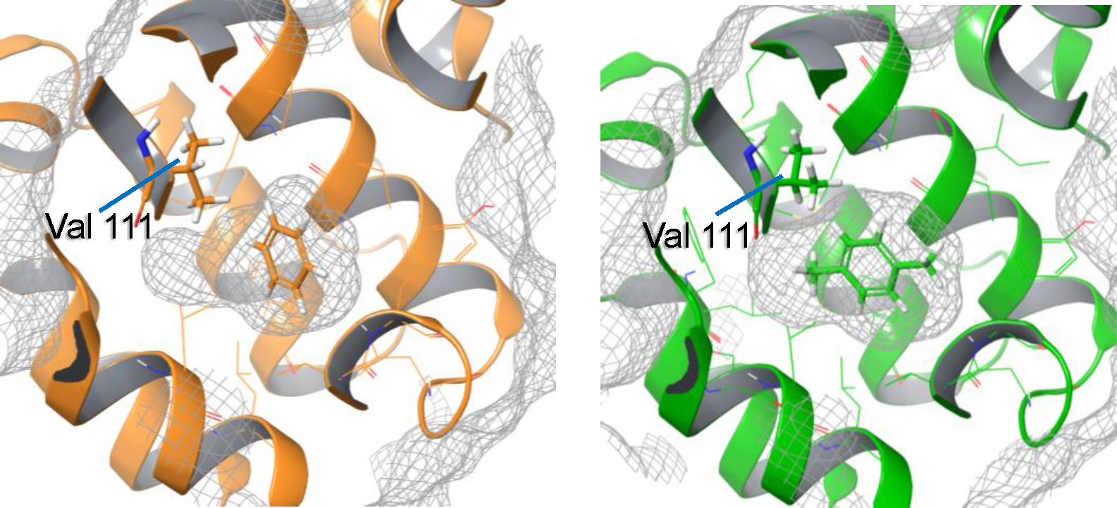
Two receptor conformations for benzene (PDBID 181L) and p-xylene (PDBID 187L) differing at Val111.¹⁵

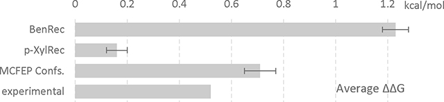
In Table 1, we summarize the results obtained if we run a conventional FEP simulation starting respectively from the benzene receptor complex (BenRec), the p-xylene receptor complex (p-XylRec), and using the HH MCFEP method in which each receptor conformation is seeded into half of the windows (with the seeded p-xylene receptor conformation created by the morphing algorithm described in Methods). Starting from the benzene receptor conformation leads to a predicted ΔΔG that is too large compared to experiment, as the penalty for forcing the p-xylene into a cavity suitable for benzene overestimates the actual penalty which arises from the reorganization energy associated with the conformational change. Starting from the p-xylene receptor, in contrast, results in a free energy difference that is too small, as the gain associated with accommodating the benzene in a smaller (and more favorable from the standpoint of protein energetics) cavity is not realized. The HH MCFEP algorithm in essence interpolates between these two values, and achieves a result that is very close to experiment.

Table 1.

Using different receptor conformers to start FEP simulations of benzene to p-xylene mutation. All units in kcal/mol and error in SEM. Experimental binding value obtained from ref¹⁶. An accompanying bar graph shown below table to visualize the ΔΔG data.

	Exp. ΔΔG	Average ΔΔG	Complex	Solvent
BenRec	0.52	1.23 ± 0.05	−10.74 ± 0.05	−11.91 ± 0.00
p-XylRec		0.16 ± 0.04	−11.75 ± 0.03	−11.91 ± 0.01
MCFEP Confs.		0.71 ± 0.06	−11.20 ± 0.06	−11.91

Figure 2 displays the distribution of dihedral values for the Val111 dihedral angle discussed above for the various simulation protocols across the FEP simulation trajectory. The key point to note is that the conventional protocols are not capable of describing the transition of the dihedral angle as the alchemical transformation parameter lambda goes from zero to one. The HH MCFEP protocol achieves the correct distribution at the endpoints by construction. While there is of course no guarantee of the precise accuracy of the distribution at intermediate lambda values, the quality of the ΔΔG prediction suggests that the HH distribution in this region is quite reasonable.

Figure 2.

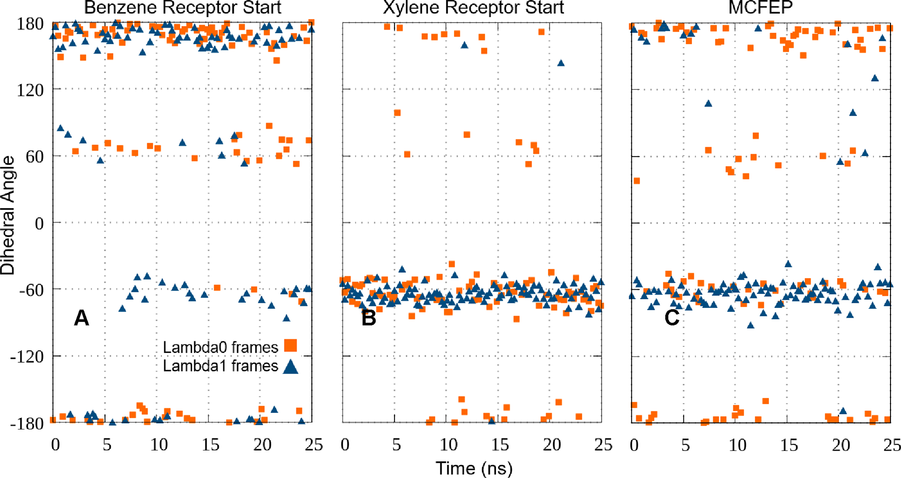
Plots of the N-CA-CB-CG1 dihedral angle at Val111 in FEP runs, first and last lambda window, various conformer setups. A. Using benzene receptor conformation to start FEP. Both windows show the angle maintaining near the −175° start. Conversion to match p-xylene crystal is insufficient. B. Using p-xylene receptor conformation to start FEP. Conversion to match benzene crystal is insufficient. C. Using benzene receptor conformation to build FEP, but applying p-xylene receptor and ligand conformation to the second half of the lambda windows to start simulation via MCFEP. Lambda0 is mainly around −175° matching the crystal conformation, and lambda1 is mostly around −60°, locally relaxed from the −35° crystal conformation. Note that due to lambda hopping, for all runs, both window ends have some mix of conformation from all the other windows, therefore the conformation from the other end also shows up.

Hsp90 Ligands

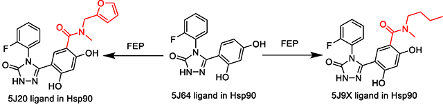
Residues 104–113 (PDBID 5J64), adjacent to the binding site of the Hsp90 chaperone protein, exhibit considerable conformation variation, indicative of the near degeneracy of the free energies of the various alternative structures. The apo Hsp90 in this region is a plastic loop-in or loop-out structure;¹⁷ furthermore, some ligands induce the formation of a helical structure. The co-crystal structures of a variety of such ligands bound to Hsp90 have been solved in a study by Amaral et. al.,¹⁸ making available systems for testing our HH method for calculating ΔΔG between a natively loop-in ligand and several natively helical ligands. This system has also been previously studied by protein reorganization FEP, although only one pair of loop-in vs helical ligands was investigated.¹⁹

In our study, for the loop-in receptor smaller ligand, PDBID 5J64 was used as a representative example (Figure 3A). For the helical receptor conformation, which accommodates larger ligands, 4 out of the 5 available such ligands in the experimental study were chosen (PDB codes 5J20, 5J9X, 5J27 and 5J82),¹⁸ all of which shared a nearly identical helical receptor conformation (Figure 3B). The remaining unchosen complex differs somewhat in the conformation of the helix. When using either the loop-in receptor (also referred to as small ligand receptor, from PDBID 5J64) or helical receptor (receptor from PDBID 5J20) to build and start a conventional FEP simulation in which a small ligand is transformed to a large ligand, the calculated ΔΔGs were either underpredicted or overpredicted, respectively (Table 2, 4 small ligand receptor and helical receptor runs). This is expected since a single receptor conformation cannot optimally accommodate both the small and large ligand types.

Figure 3.

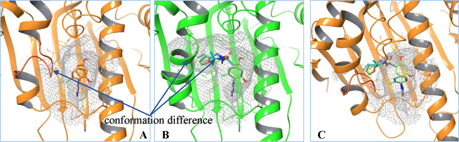
A.small ligand binding in an apo-like loop-in conformer. B.large ligands inducing and binding in a helical shape receptor. C.if superimposing or attempting to fit the large ligands into the loop-in receptor, it will protrude into the molecular surface of the protein.

Table 2.

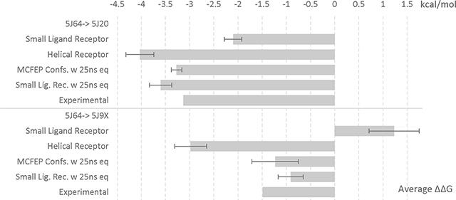
5J64 ligand to 5J20 and 5J9X ligands FEP. All units in kcal/mol and error in SEM. An accompanying bar graph shown below table to visualize the ΔΔG data.

5J64-> 5J20	Exp. ΔΔG	Average ΔΔG	Complex	Solvent
Small Ligand Receptor	−3.13	−2.10 ± 0.18	31.14 ± 0.20	33.23 ± 0.03
Helical Receptor		−4.03 ± 0.29	30.04 ± 0.29	34.07 ± 0.02
MCFEP Confs. w 25ns eq		−3.27 ± 0.11	29.97 ± 0.12	33.23
Small Lig. Rec. w 25ns eq		−3.6 ± 0.23	29.63 ± 0.21	33.23 ± 0.03
5J64-> 5J9X
Small Ligand Receptor	−1.49	1.23 ± 0.52	35.41± 0.49	34.19 ± 0.04
Helical Receptor		−2.98 ± 0.33	32.96 ± 0.32	35.94 ± 0.02
MCFEP Confs. w 25ns eq		−1.23 ± 0.48	32.96 ± 0.48	34.19
Small Lig. Rec. w 25ns eq		−0.91 ± 0.26	33.28 ± 0.24	34.19 ± 0.04

Table 4.

5J64 ligand to 5J27 and 5J82 ligands FEP. All units in kcal/mol and error in SEM. Modified small molecule dihedral parameters. An accompanying bar graph shown below table to visualize the ΔΔG data.

5J64 ->5J27	Exp. ΔΔG	FF offset corr. avg. ΔΔG	Average ΔΔG	Complex	Solvent
Small Ligand Receptor	0.12	2.16	2.95 ± 0.28	43.00 ± 0.26	40.05 ± 0.02
Helical Receptor		-0.9	-0.11 ± 0.17	49.89 ± 0.18	50.00 ± 0.01
MCFEP Confs. with 25ns eq.		0.75	1.54 ± 0.45	41.60 ± 0.45	40.05
Small Lig. Rec. with 25ns eq.		0.97	1.76 ± 0.32	41.81 ± 0.33	40.05 ± 0.02
5J64 ->5J82
Small Ligand Receptor	1.17	3.11	4.16 ± 0.23	34.43± 0.21	30.28 ± 0.02
Helical Receptor		-0.36	0.69 ± 0.02	30.97 ± 0.02	30.29 ± 0.01
MCFEP Confs. with 25ns eq.		2.03	3.08 ± 0.42	33.35± 0.42	30.28
Small Lig. Rec. with 25ns eq.		2.9	3.95 ± 0.50	34.23 ± 0.51	30.28 ± 0.02

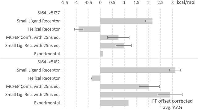
A challenging feature of the present problem is that an attempt to place the large ligands in the smaller cavity loop-in receptor conformation inevitably results in steric clashes (see Figure 3C). Ordinarily, if a small fraction of the Hamiltonian of ligand B replaces the same fraction of the ligand A Hamiltonian during the alchemical transformation, the system will adopt a conformation close to that of ligand A conformation, accepting an inferior environment for the ligand B component of the mixed Hamiltonian because it is small, and avoiding clashes with ligand B via minor adaptations of atomic positions. Indeed, this reasoning is a principal rationalization for using the HH multiconformational protocol. In the present case, the exceptionally poor fit of the large ligands into the small cavity makes such minor adaptations much more difficult to achieve than is usual. We found that for the most part this problem can be effectively addressed by utilizing an extended equilibration period before the FEP production calculation starts, which enables in windows 2–6 the more substantial adaptations of the small cavity starting point to the larger ligand to be achieved. Windows 7–12 already have the large helical cavity to begin with as mandated by the HH MCFEP protocol. An important point to note is that the requirement for this extended equilibration could be inferred without knowing the experimental binding affinities, simply by detecting the significant and unavoidable clashes that are manifested upon initial placement of the large ligand in the small ligand cavity.

We note that the extended equilibration period could also be used during a conventional FEP simulation starting from the small ligand conformational state. We carried out such an experiment and the binding free energy prediction was in fact improved, however the results were not as good as that of MCFEP, and for 5J64->5J20 (Table 2 row 5) the binding free energy was overcorrected as compared to experiment. Examining the energy of this overcorrected calculation over time, we found that the initial 25ns relaxed the system into a metastable state, such that the 25ns period afterwards for collecting energies was very unstable in terms of ΔG. Additionally, the helical conformer was not found by the FEP simulation. In contrast, the 25ns of FEP production using the HH MCFEP protocol was very stable in energy and clearly in the correct conformational state for each lambda end point. See SI Figure S1 for the energy plots.

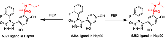
The 5J27 and 5J82 ligands both contain a sulfonamide group that form an intramolecular H-bond with an ortho OH when free in solution (SI Figure S4). When bound in the receptor pocket, this OH group is rotated 180°, where it is observed to interact with one of two buried waters in the region and at an energy cost of approximately 3 kcal/mol based on implicit solvent QM calculations. Using the original OPLS4 parameters however, it is estimated that there is no energy cost of this rotation in aqueous solution (SI Table S1). Conventional FEP test runs between pairs of amide and sulfonamide containing ligands, both of which are native to the same helical receptor (and therefore a conformation change is not relevant), show the binding affinities being significantly overpredicted by approximately 3–4 kcal/mol (SI Table S2). Consequently, force field dihedral parameters for this motif were modified to apply an additional penalty of approximately 3 kcal/mol to this rotation.

To test the dihedral correction, the same FEP tests were run again with the modified dihedral parameters (Table 3). Results were significantly improved even though not perfect, yielding average residual errors of respectively 0.79 and 1.05 kcal/mol for each ligand versus experiment, which we attribute to remaining imperfections in the force field.

Table 3.

5J20 and 5J9X ligands to 5J27 and 5J82 ligands FEP runs with modified small molecule dihedral parameters. Runs involving both sulfonamide ligands of 5J27 and 5J82 are now slightly underpredicted of the binding by 0.79 and 1.05 kcal/mol, respectively. All units in kcal/mol and error in SEM.

	Exp. ΔΔG	Average ΔΔG	Complex	Solvent	Residual error
5J20 ->5J27	3.25	4.01 ± 0.30	19.05± 0.26	15.05 ± 0.05	0.76
5J9X ->5J27	1.61	2.44 ± 0.24	14.28 ± 0.28	11.84 ± 0.04	0.83
5J20 ->5J82	4.30	5.10 ± 0.11	0.62 ± 0.12	−4.48 ± 0.07	0.80
5J9X ->5J82	2.66	3.95 ± 0.07	−3.8 ± 0.04	−7.75 ± 0.04	1.29
Average Residual Error	5J27				0.79
	5J82				1.05

Running the MCFEP protocol using the modified force field parameters, and further offsetting the remaining force field level errors via empirical correction based on the residual errors of 0.79 and 1.05 kcal/mol, the differences to experiment are 0.63 and 0.86 kcal/mol, within the normal error margin of FEP, and substantially improved compared to results using a single conformer conventional FEP simulation (Table 4).

Mutation in the ACE2/RBD protein-protein complex

In a previous study, we used FEP to evaluate the effect of mutations on binding between a receptor binding domain (RBD) of SARS-CoV-2 spike protein and a human angiotensin converting enzyme 2 (ACE2).²⁰ While the overall prediction accuracy across various mutations was good (RMSE=0.8), a single outlier, the Q498R mutation of RBD, had the destabilizing effect overpredicted by more than 2 kcal/mol compared to the near neutral experimental ΔΔG value (0.2 kcal/mol).²⁰ Table 5 (top) shows a gradual decrease in the predicted change in binding affinity upon mutation as the length of the simulation increases, yet, even at 300ns the result is not fundamentally different, and the mutation is still predicted as largely destabilizing (ΔΔG=1.9 kcal/mol). Of note, running a 300ns FEP simulation for such a large complex is computationally intensive requiring ~20 days of wall time on 4 A4000 NVIDIA GPUs; hence, not commonly done.

Table 5.

RBD/ACE2 Q498R mutation binding ΔΔG, experimental ΔΔG=0.2, all units in kcal/mol.

Q498R (Forward run)	ΔΔG	Complex	Solvent
50ns	2.77	−85.83	−88.60
100ns	2.34	−86.35	−88.69
200ns	1.93	−86.83	−88.76
300ns	1.86	−86.88	−88.74
R498Q (Reverse run)
50ns	0.40	−44.82	−45.22
100ns	−0.02	−45.23	−45.21

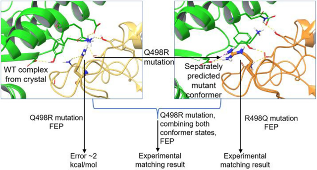
Analysis of the forward FEP trajectories of the Q498R mutant revealed that the most prevalent state had unfavorable polar-hydrophobic interactions (Figure 4, state A) likely contributing to the destabilizing ΔΔG value predicted by FEP (Table 5). A single alternative conformation found in the 100% mutant window FEP trajectory, while not being dominant in population, arguably had more stabilizing interactions (Figure 4, state B). Therefore, we hypothesized that state B was the energetically favored state of the mutant antibody-protein complex. From the 100% mutant window, the first occurrence of state B was visually picked out to start a reverse FEP simulation (R498Q), and the results matched experiment within 0.2 kcal/mol (Table 5 bottom).

Figure 4.

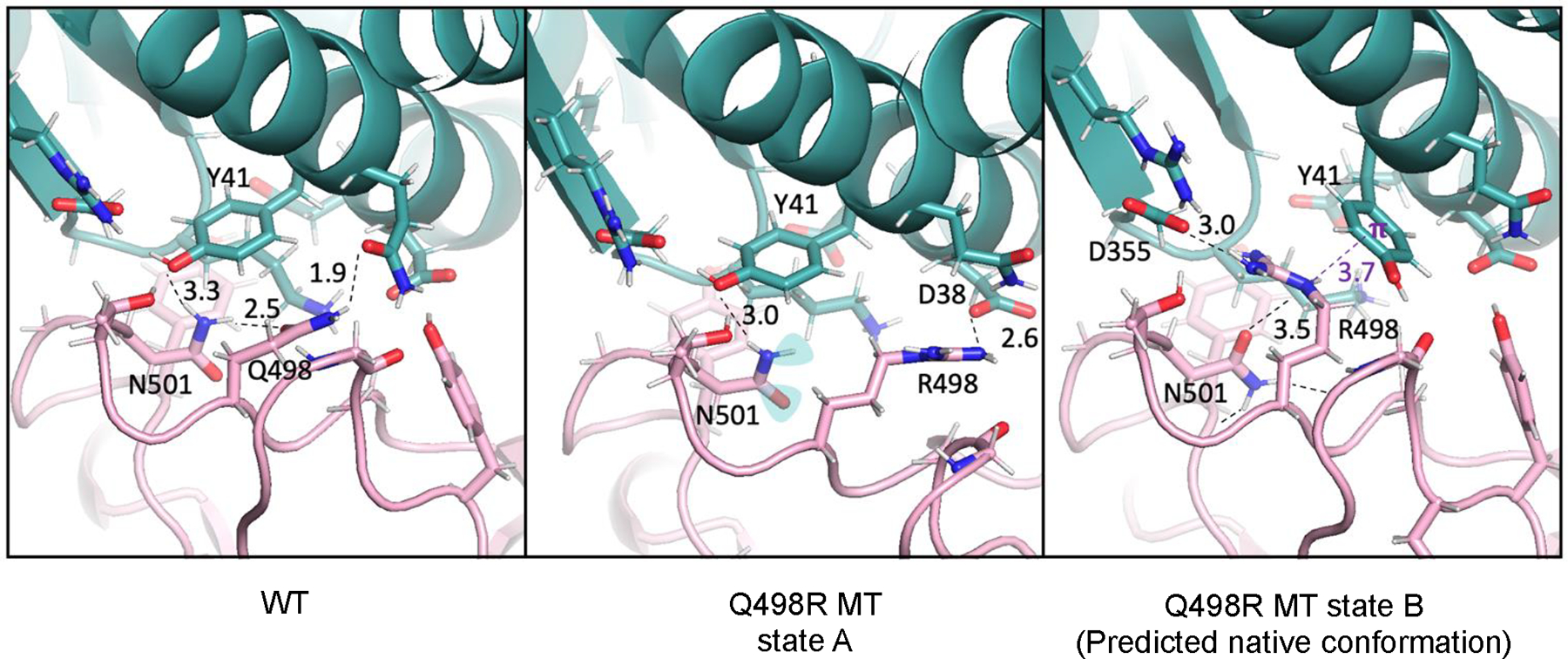
RBD(pink)/ACE2(cyan) interactions involving RBD residues in the native Q498 state (left panel, PDBID 6M0J), the Q498R mutant state prevalent in a forward run FEP trajectory (middle panel) and the alternative mutant Q498R state prevalent in the REST2 REMD trajectory (right panel). State A, which is structurally similar to the starting WT conformation, contains destabilizing interactions, N501 with unsatisfied polar groups. State B contains stabilizing interactions, R498 head group and the Y41 aromatic ring involved in cation-pi-stacking (purple) and a hydrogen bond between N501 carbonyl and R498 (black dashed line). Distances in Å.

We further conducted independent REMD simulations with enhanced sampling via REST2 with hot atoms on and around R498, and used either state A or state B as a starting geometry. The results of three independent runs reproducibly indicated that state B has a better occupancy than state A, regardless of the starting point (Table 6); thus, confirming our conjecture that state B is the lowest free energy conformer for the Q498R mutant. If state B were properly sampled as the dominant pose in FEP, the Q498R mutation should yield the binding free energy change for the mutation in better agreement with the experiment. Of note, sampling using independent REST2 REMD runs is more effective than REST2 sampling in FEP, even when the REST2 hot atoms are the same. This is because REST2 REMD implemented in FEP exchanges between different alchemical states, whereas independent REMD exchanges in the 100% mutant state only.

Table 6.

REMD simulations for state stability analysis. 50ns x3 runs each, 10–50ns portion of frames collected for population analysis. D38–498R or D355–498R contact (3Å cutoff) as identifier for A or B.

	State A start		State B start
	Fraction of A	Fraction of B	Fraction of A	Fraction of B
Run1	0.14	0.10	0.21	0.63
Run2	0.04	0.43	0.35	0.36
Run3	0.07	0.20	0.27	0.54

In the forward FEP simulation the sidechains in the vicinity of the Q498R mutation are trapped in the conformation reminiscent of WT (Figure 4, state A). To reach state B from state A, the arginine sidechain generated by the protein mutation builder needs to cross over and partially displace Y41 while a sidechain of N501 gets flipped. These events happened rarely in the FEP trajectory, resulting in underrepresentation of state B. In contrast, in the reverse simulation starting from state B, once a larger sidechain (Arg) got mutated into a smaller one (Gln), both Q498 and Y41 relaxed to WT-like state with ease, suggesting a smaller barrier due to less steric hindrance. As a result, the reverse simulation achieved correct end states for both Q498 and R498, and, thus, good agreement with the experiment.

To test whether the forward simulation can possibly achieve the correct answer, our HH MCFEP method was applied. Building the FEP simulation from the crystal complex, the second half of the windows were morphed into the state B conformer. By 25ns, the same simulation time we used for our other systems, the error reduced to ~0.4 kcal/mol (Table 7), thus, markedly improving agreement with the experiment compared to the conventional forward FEP simulation starting from the crystal complex (Table 5). The cumulative energy plot over time for the complex leg shows that the MCFEP simulation is stable and converged (SI Figure S2).

Table 7.

MCFEP calculation of the Q498R mutation in the RBD/ACE2 complex using separately predicted state B conformer for the Q498R mutant. All units in kcal/mol and error in SEM.

	Exp. ΔΔG	Average ΔΔG	ΔΔG	Complex	Solvent
Run 1			−0.37	−89.04	−88.67
Run 2			0.00	−88.67
Run 3			−0.32	−88.99
	0.2	−0.23 ± 0.09		−88.90 ± 0.09

It is noteworthy that this is a case where a computationally predicted structure, rather than an experimentally derived structure, is used as a representation of the final state. This is a situation that arises frequently in ongoing drug discovery projects, where obtaining crystal structures can be time consuming and expensive. The success of this approach is encouraging with regard to deployment of the MCFEP using computational structure prediction, although many more test cases will need to be examined in order to determine the robustness of such a methodology.

Abl kinase ligands

Like many kinases, Abl kinase exhibits significant conformational plasticity. A key region where substantive conformational change can be observed as a function of ligand binding is the P-loop, which is proximate to the kinase ATP binding pocket region. Depending upon the ligand, the P-loop can either adapt a fully extended beta strand conformation (Figure 5, green) or become collapsed and loop-like (Figure 5, orange). Here we study the relative binding free energy difference between ligands dasatinib and tozasertib. Dasatinib binds to the extended beta-strand conformation,^{19, 21, 22} while tozasertib induces a collapse to the loop-like conformer.^{23, 24} In the absence of a ligand, the extended P-loop is suggested to be the more energetically favored conformer from an analysis of various apo structures of kinases,^{25, 26} and from calculation.¹⁹

Figure 5.

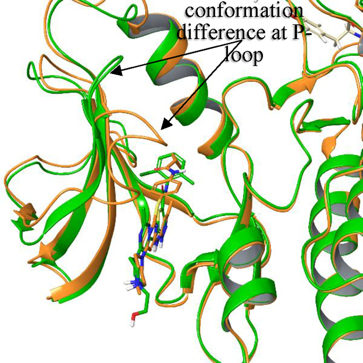
Superimposed structures of dasatinib-Abl complex (PDBID 2GQG, green) and tozasertib-Abl complex (PDBID 2F4J, orange). 2GQG is re-refined at the P-loop from the raw diffraction data, as the original deposit had no electron density in the tip residues of 250–254, but the difference density suggested an extension of the beta strand, i.e. extended P-loop. Also, mouse Abl2 with the same ligand bound had an extended P-loop (PDBID 4XLI), and was used as a homology model in a prior study for dasatinib FEP calculations,¹⁹ instead of the original 2GQG deposited structure.

Dasatinib, a second generation Abl kinase inhibitor, has substantially enhanced binding affinity as compared to first generation and other second generation molecules.²⁷ This enhanced binding affinity of dasatinib is suggested to be achieved primarily because the apo P-loop is essentially unchanged after dasatinib binding, avoiding a significant reorganization free energy cost, unlike other molecules that do cause a change, including tozasertib.¹⁹ Tozasertib, while active against T315I mutant Abl when dasatinib is not, binds to WT Abl significantly more weakly than does dasatinib, consistent with the fact that the P loop conformation observed in the tozasertib complex structure is quite different from the conformations observed in both the dasatinib-bound and apo structures. In ref. ¹⁹, an FEP algorithm specialized to the calculation of protein reorganization energy was used, in conjunction with absolute binding free energy FEP methods (ABFEP),²⁸ to compute the total binding affinities of dasatinib and tozasertib. This approach is likely reasonably accurate and produces values of the total binding free energies for dasatinib and tozasertib, comprised of the absolute binding free energy of each ligand from their native receptor conformer, and an additional protein reorganization free energy from the apo state, applicable to tozasertib. However, it is also quite expensive computationally. In the present section, we explore the use of both single conformation and multiconformation FEP calculations to determine the relative binding affinity of the two complexes. Due to the nature of relative binding FEP, the apo protein is not required or involved in the calculation.

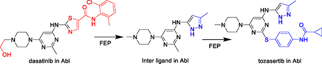
The ligands tozasertib and dasatinib, shown in Table 8, are chemically quite different from each other, to the point where a direct FEP transformation between them would present technical difficulties. In order to facilitate the alchemical modeling, we define an intermediate molecule resembling the common substructure of dasatinib and tozasertib, denoted “Inter” below, and break up the FEP calculation into two steps, first transforming from dasatinib to Inter, and then from Inter to tozasertib. The identity of Inter and its assumed binding conformation are irrelevant in principle to the computed thermodynamics of dasatinib to tozasertib free energy changes, as the free energy is a path independent state function.

Table 8.

Dasatinib (das) to tozasertib (toz) ΔΔG FEP calculation (via an intermediate ligand) using either the dasatinib receptor or the tozasertib receptor, as well as applying the MCFEP conformers. All units in kcal/mol and error in SEM. IC50 value from refs ^{19, 29}, ABFEP+protein reorganization FEP value from ref ¹⁹. An accompanying bar graph shown below table to visualize the ΔΔG data.

	Average ΔΔG	Complex	Solvent
Das ->Inter (Das Rec)	10.68 ± 0.68	−12.73± 0.69	−23.41 ± 0.03
Das ->Inter (Toz Rec)	10.63 ± 0.52	−16.02 ± 0.49	−26.65 ± 0.03
Inter ->Toz (Das Rec)	−2.13 ± 0.20	−2.03± 0.23	0.10 ± 0.03
Inter ->Toz (Toz Rec)	−5.85 ± 0.17	−13.07 ± 0.17	−7.22 ± 0.01
DasRec Total	8.46 ± 0.36
TozRec Total	4.81 ± 0.26
MCFEP Confs. Inter ->Toz	−3.36 ± 0.18	−2.84 ± 0.20	0.10
MCFEP Confs. Total	7.32 ± 0.36
Reference ΔΔG	From IC50 (beyond assay limit) >3.9 From ABFEP + Protein Reorg. FEP 6.2 ± 0.8

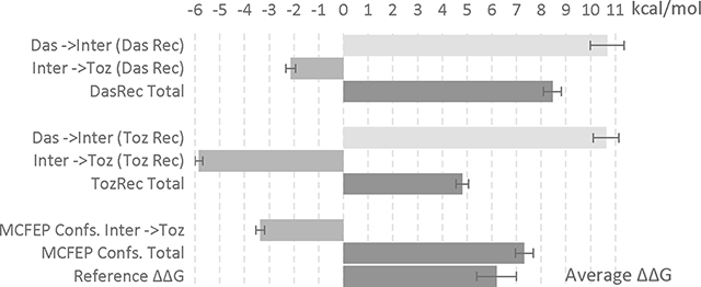
As we have chosen Inter to be a common substructure of dasatinib and tozasertib, we are able to place it in a suitable low energy conformation in both the tozasertib and dasatinib structures, simply by superimposing it on the original ligands. In order to compare the effect of the two different receptor conformers, we explore two thermodynamic pathways. In the first, we start from dasatinib in its native structure and receptor (DasRec) environment, transform the ligand to Inter in the DasRec environment, and then transform from Inter/DasRec to tozasertib in DasRec. In the second pathway, we start from dasatinib superimposed to the native complex structure of tozasertib, transform to Inter in the native tozasertib receptor (TozRec) environment, and finally transform from Inter/TozRec to tozasertib in TozRec (see SI Figure S3 for illustration of pathways).

The results of using single conformation FEP to evaluate these two pathways are shown in Table 8, first 6 rows. For the first pathway utilizing the DasRec environment, the total results are too positive as compared to the protein reorganization FEP/ABFEP calculation (which we use as a benchmark); for the second pathway utilizing the TozRec environment, the total results are not positive enough. The difference in the sign of the error arises because in the first pathway, tozasertib does not have the correct native receptor conformer, whereas in the second pathway dasatinib does not have the correct native receptor conformer.

In deploying our MCFEP approach, we need to correct the step in which either das is in the wrong state, or toz is in the wrong state. Since free energy is a state function, even if the Inter is also somewhat incorrect, going from the das(correct) -> Inter(wrong) -> toz(correct) does not change the overall das to toz ΔΔG. Nevertheless, described in SI Figure S3, we determined Inter(d) is lower than Inter(t), therefore we chose to correct the inter(d) to toz step because the other choice would have two unfavorable ends and may give extra noise.

Utilizing the HH MCFEP methodology to evaluate the inter(d) to tozasertib step in the first path, the overall ΔΔG is in between the overpredicted and underpredicted single conformer FEP results for the two paths, and within a normal FEP error margin of the ABFEP with protein reorganization energy result (Table 8). While the correction to single conformation FEP is not particularly large, the overall alchemical transformation and structural change are complex, so the validation of the HH MCFEP approach for this problem suggests that the domain of applicability of the methodology is substantial (although many more test cases will be needed to verify this hypothesis explicitly).

Final overall comparison of MCFEP with conventional FEP using enhanced sampling by extended hot atoms REST2

To address the long standing issues of conformation change, enhanced sampling by REST2 has already been commonly used in FEP simulations.^{4, 9, 12, 30, 31} Also the standard setup in FEP+, the REST2 hot atoms are by default limited to the alchemical ligand atoms only. As mentioned in the initial publication of implementing REST2 in FEP, the choice of hot atoms is a balance between more sampling but more noise against less noise.¹² All the results in Tables 1–8 have the default hot atoms of ligand alchemical atoms only. We noticed that in the initial publication, in the T4 lysozyme ligand pair of benzene to p-xylene, the hot atoms were expanded to Val111 in the protein, and FEP results matched experimental results precisely, as a successful demonstration of REST2 in FEP. To better evaluate MCFEP, we decided to compare MCFEP results to FEP with the hot atoms expanded to known conformation change regions as well, in all our systems and ligand pairs. We run this comparison in the belief that extended hot atoms REST2 is the best sampling within FEP currently available. Results are shown in Table 9. The ΔΔG avg. columns of Table 9 are visualized in Figure 6.

Table 9.

Comparing MCFEP with FEP extended REST2 hot atoms. FEP started from the smaller ligand receptor conformer for T4 lysozyme and Hsp90 systems, from the WT crystal for RBD/ACE2, and from the das rec conformer for the Abl system, respectively. Length of simulation is 25ns for all except the Q498R conventional FEP run being 100ns. In the four Hsp90 system runs, the same 25ns pre-lambda hopping equilibration was equally applied to both MCFEP and FEP with extended REST2 hot atoms.

System and mutation	Exp. ΔΔG	MCFEP				Conventional FEP with extended REST2 hot atoms on conformation change residues, single conformer start
		ΔΔG avg.	ΔΔG	Complex	Solvent	ΔΔG avg.	ΔΔG	Complex	Solvent
T4 lysozyme	0.52	0.71	0.57	−11.34	−11.91	0.56	0.58	−11.33	−11.91
benzene -> p-xylene		±0.06	0.78	−11.13		±0.01	0.56	−11.35
			0.78	−11.13			0.53	−11.38
Hsp90	−3.13	−3.27	−3.38	29.85	33.23	−3.20	−4.02	29.21	33.23
5J64 -> 5J20		±0.11	−2.99	30.25		±0.35	−3.02	30.21
			−3.43	29.8			−2.55	30.68
5J64 -> 5J9X	−1.49	−1.23	−2.2	31.99	34.19	−0.59	0.13	34.32	34.19
		±0.48	−1.32	32.87		±0.30	−0.86	33.33
			−0.16	34.03			−1.04	33.15
5J64 -> 5J27 (FF offset corrected)	0.12	0.75	1.84	41.89	40.05	1.23	0.92	40.94	40.05
		±0.45	0.04	40.09		±0.19	1.07	41.15
			0.39	40.44			1.69	41.74
5J64 -> 5J82 (FF offset corrected)	1.17	2.03	2.05	32.33	30.28	3.07	2.76	33.07	30.28
		±0.42	1.12	31.39		±0.36	3.94	34.18
			2.91	33.19			2.50	32.78
RBD/ACE2	0.2	−0.23	−0.37	−89.04	−88.67	2.38	2.48	−86.21	−88.69
Q498R		±0.09	0.00	−88.67		±0.16	2.01	−86.68
			−0.32	−88.99			2.65	−86.04
Abl		−3.36	−2.94	−2.84	0.1	−1.62	−1.82	−1.72	0.1
Inter -> Toz (DasRec Start)		± 0.18	−3.44	−3.34		± 0.10	−1.40	−1.30
			−3.7	−3.60			−1.63	−1.53
Das-Inter-Toz Total	>3.9a 6.2±0.8b	7.32 ±0.36				9.06 ±0.35
	MUE		0.52				1.28
	RMSE		0.62				1.61
	R2		0.99				0.96

^aBeyond assay limit.

^bFrom ABFEP with protein reorg. FEP included.

Figure 6.

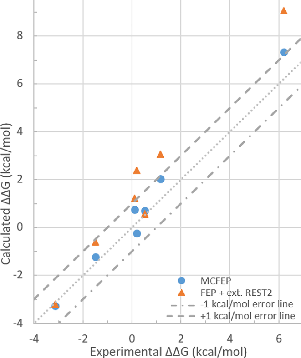
Experimental vs calculated average ΔΔG values from Table 9, with ±1 kcal/mol error margin shown within dashed lines.

The results indicate that REST2 extended hot atoms worked very well for the T4 lysozyme system, the one with the simplest conformer change, as we reproduced the same results as reported previously.¹² Val111 was properly rotating even though starting from one conformer only. However, for any of the more complicated conformation changes, extended hot atoms did not show any improvement compared to only hot atoms in the ligand alchemical part, as shown in the previous tables 1,2,4,5 and 8. For the 5J64 to 5J20 ligands REST2 with extended hot atoms runs, even though the results matched experiment, this was the result of alternative metastable states and the correct helical conformation was not found for the 5J20 ligand complex, similar to the result from Table 2. The calculated free energies over time were not stable or converged (see SI Figure S1 for plots).

Finally, the mean unsigned error (MUE) against experimental values across the 4 systems for MCFEP vs. conventional FEP simulation is 0.52 vs 1.28 kcal/mol, or in terms of RMSE, 0.62 vs 1.61 kcal/mol. This is a substantial and systematic reduction in the error across a range of different binding affinity calculations. As successful use of FEP calculations in practical drug discovery efforts is often contingent upon reduction of the prediction errors to less than ~1 kcal/mol,³² the improvements demonstrated here for MCFEP are likely to be highly relevant to such practical applications. The results of each individual run are reported in SI Tables S3–10.

Discussion

We have investigated above the application of the HH implementation of a novel multiconformational FEP methodology (MCFEP) to a diverse and challenging range of protein-ligand systems. Unlike conventional FEP where all lambda windows are seeded with the same complex conformation, different lambda windows are started with different protein and ligand conformations in MCFEP and the input conformations for the physical end points are guided by either experimental structures or computational prediction. We categorize the sampling under MCFEP into two types: 1) When continuous MD can sample the transition between different conformations; and 2) When continuous MD under a certain temperature and condition cannot sample the transition between different conformations. In scenario 1), by providing the preferred conformers to start, the effect of HH MCFEP is essentially speeding up the equilibrium process by starting at or close to equilibrium.¹² In scenario 2), even when continuous MD cannot sample the transition, HH MCFEP is making a simplified, but apparently often reasonable, approximation of the equilibrium windows ratios. Both types of scenarios are seen in our study here. Two of the four systems studied in this work have seen continuous MD transition between conformers, namely the T4 lysozyme and RBD/ACE2 Q498R mutation. When the T4 lysozyme simulation started from a single conformer, the other conformer was seen (Figure 2). The Q498R mutant state B (Figure 4), later determined as the native state, was initially found in a conventional FEP simulation starting from the WT conformer. Only side chain changes were involved in these two systems. The other two systems of Hsp90 and Abl did not show a transition between conformers in continuous MD. Backbone changes were involved in these two systems. HH MCFEP provided sufficient accuracy for all four systems and cases.

There will indeed be complicated cases where the transition barrier is too high for continuous MD to cross on a practical time scale, and which at the same time the equilibrium distribution ratio of windows for the two conformers is not 1:1. In these cases where a non 1:1 equilibrium ratio is needed, techniques like combining HH MCFEP with extended hot atoms REST2 to help the transition occur, or independently searching at around mid-point lambda values and determining the actual ratio of windows (or switching point) (i.e. non-HH MCFEP) are expected to improve accuracy.

Practically, our study results here seem to indicate that the 1:1 approximation is likely to be sufficient accuracy for many cases. Specifically, significant reductions in the error as compared to single conformation FEP were obtained, with an absolute error within the statistical norm for FEP calculations where conformational change is not an issue (on the order of 1.1 kcal/mol as per ref. ¹³). In two of the FEP calculations for the Hsp90 system, a significant portion (0.79 and 1.05 kcal/mol) of the residual error arises from unresolved problems with the force field description of the sulfonamide and adjacent OH torsion. If the results are corrected for this force field error, then the HH/MCFEP results for both of the problematic Hsp90 cases are within the 1.1 kcal/mol error range, and the performance of the MCFEP is superior to that of the single conformation FEP.

The MCFEP approach requires that conformational endpoints for the alchemical ligand target and/or protein mutation target be determined. If high resolution experimental structures are available for both endpoints, there is no problem in satisfying this requirement. However, in practical drug discovery applications, many important use cases will be ones where the conformational end point in the context of the target ligand or protein mutation is not known. In these cases, structural models must be obtained computationally. The great strength of the MCFEP approach presented here is that, rather than having to rely on the FEP simulation itself to converge to the correct endpoint structure as the FEP window approaches lambda=1, alternative algorithms with a superior ability to rapidly search phase space and overcome energy barriers can be deployed. These include conformational search methods employing continuum solvation models (e.g. the Prime loop prediction algorithm³³), induced fit docking (e.g. the Schrodinger IFD-MD methodology³⁴), replica exchange MD as was used above for the RBD Q498R mutation, informatics based structure prediction algorithms such as are used in Alphafold2³⁵ and related programs, and machine learning-based algorithms to accelerate conformational sampling. Multiple methods enumerated above may also be combined to form workflows as is already done in IFD-MD.

An illustrative application where we believe that MCFEP will be particularly useful is in antibody optimization of antibody-receptor binding affinity. We have recently shown that FEP methods can be quite accurate in predicting the effects of mutation on the antibody receptor binding free energy.^36–38 However, current technology assumes minimal changes in protein conformation upon mutation. This assumption is not always valid as we have seen above for the RBD Q498R mutation. Assuming that a reliable approach to predicting the structure of the mutated antibody (in both the antibody receptor complex and in the isolated antibody) can be developed using the tools cited above, computational antibody engineering could be brought to a new level of robustness and accuracy.

Conclusions

We have described a novel approach to free energy perturbation simulations, MCFEP, in macromolecular systems which is capable of achieving accurate results when there are significant conformational changes between the two alchemical endpoint states A and B. A simple implementation, which half of the windows are seeded with conformation A and half with conformation B, has been shown to produce high quality results for free energy changes for systems involving both protein-ligand binding and the effects of mutation on protein-protein binding. One of the most important advantages of MCFEP is that it allows any method of structure determination to directly help the FEP simulation, as we have demonstrated use of both experimental and predicted structures. One can easily test and compare as many conformers as a project needs, especially if prediction provides multiple candidates for the target end conformer. The computational cost of the methodology is comparable to that of a conventional, single conformation FEP simulation. MCFEP was tested on a diverse set of four increasingly complex systems, containing seven binding pairs in all. Compared to the best current FEP technology of using extended REST2 sampling on regions of known conformation change, MCFEP performed better in 6 of the 7 pairs, with only the simplest conformation change case yielding a similar result. Compared to FEP using REST2 hot atoms on only the ligand alchemical atoms, as is the standard FEP setup in many cases like FEP+, MCFEP performed better in all pairs. Compared to experiment, after removing FF errors for 2 of the 7 pairs, MCFEP matched experimental results within 1 kcal/mol for all pairs. The RMSE to experiment was 0.62. The same measurements using conventional FEP with extended hot atoms gave an RMSE of 1.61.

As has been discussed above, there are a number of directions in which technical improvements can be made, including the mechanics of the MCFEP protocol, the algorithms used to generate end point states if an experimental structure is not available, and as well as exploring non-HH MCFEP. We believe that progress in both of these areas will result in a robust platform for applying FEP in a wide range of use cases which are difficult or intractable with currently available methods. In conjunction with scaling up the number of retrospective test cases and validation via prospective predictions, MCFEP can evolve into a powerful tool that is routinely used in drug discovery projects and more generally to explore free energy changes in complex biological and materials science systems.

Methods

Preparing custom conformer lambda windows for MCFEP

The custom conformers were seeded through the multisim workflow of the Schrodinger Suite and FEP+ without need of any internal modifications to the public release. Version 2022–3 was used, while other versions will work as well. A flowchart of the process is provided in Figure 7. The idea was starting an FEP simulation 1 from the known conformer of the WT, use the stop{} keyword to stop the multisim workflow after the first 100 ps of equilibration, and then replace the second half of the lambda windows with the known mutant conformer.

Figure 7.

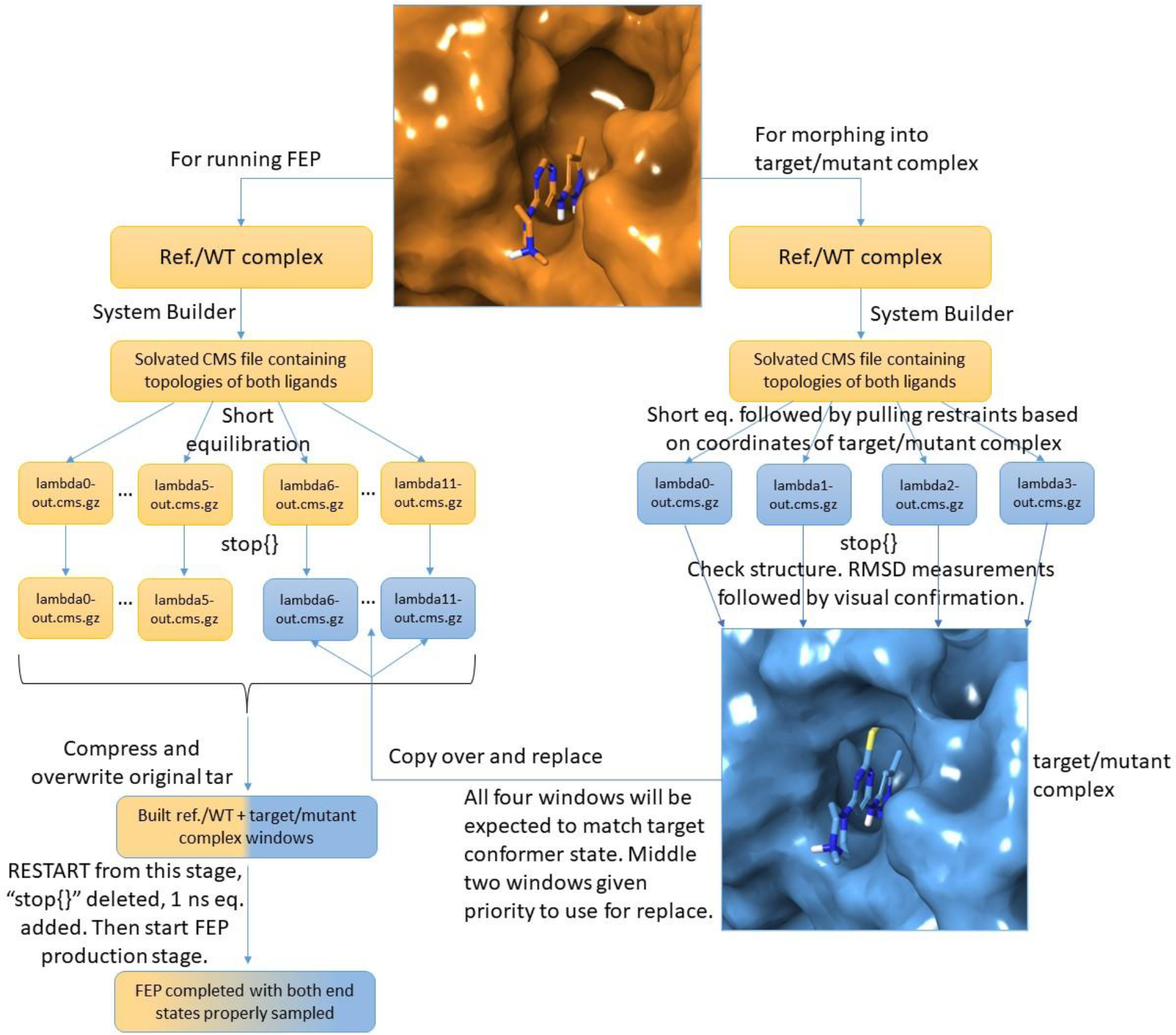
Schematic workflow for starting MCFEP with the current public releases of the Schrodinger Suite. The “Ref.” refers to the ligand which is alchemically changed away from and which the ΔG is compared against in small molecule FEP. The “WT” refers to the same reference but in the context of protein FEP.

The mutant conformer itself was prepared in the following way: starting another FEP simulation 2 from the same WT input structure file, after the first equilibration stage, a pulling stage was inserted such that positional restraints on all solute atoms except hydrogens would pull the WT atom coordinates to match that of the desired mutant conformer. As the pulling target, coordinates of the mutant conformer were extracted from a PDB version of the mutant structure, written into multisim harmonic restraints format with a force constant of 5 kcal/mol/Ų, and inserted into the new pulling stage of the workflow. This target PDB file was saved after alignment to the WT conformer, so that regions other than the conformational change region will have very little movement. The rezero option in the system builder stage was turned off. To minimize the time of this pulling stage, the minimum number of lambda windows, 4, was used, and pulling time was set to a nominal 90 ps, even though the solute movement was complete within 24 ps. After this stage is complete, the stop{} command is used again. To confirm the precise match of the morphed conformer with the target, visual inspection was performed. For convenience, before the visual inspection, RMSD measurements to the target PDB for the conformational change region residues were performed on all 4 windows using cpptraj.³⁹ The smallest RMSD window was chosen with windows 2 or 3 given priority so both alchemical molecules exist (avoiding clashes including with water when later applying the coordinates to other lambda values). In this way, visual inspection was only needed on one or two windows.

Once the precisely matching window to the target is determined, the output .cms file of this stage is copied over to FEP simulation 1, replacing the .cms files of the second half of the windows in the last stage before the workflow was stopped. In this way, we have achieved identical topologies and water molecules between the first and second half of the windows in simulation 1. The multisim workflow was restarted from this stage. Due to the fact that the conformer was established through pulling, an unrestrained 1 ns additional relaxation was supplied in the next stage of GCMC solvation. For the Hsp90 ligands, considering the clashing size of the small molecule pocket compared to the large ligand, a longer 25 ns relaxation (NVT, 310K, Langevin thermostat tau=100) was used, with the 5J64 ligand and protein residues 48, 54, 93 held restrained on heavy atoms. After the relaxation stage, the lambda hopping stage was run as usual by default setups including lambda exchange.

A general scheme for describing the complex and solvent leg calculations in FEP and MCFEP is provided in Figure 8. For more detailed descriptions of the lambda hopping stage and all the other stages, including preparing the ligands and proteins, see SI. Two examples runs, one for small molecule FEP, one for protein FEP, are provided on the Github repository github.com/JL2021MD/MCFEP for users to follow.

Figure 8.

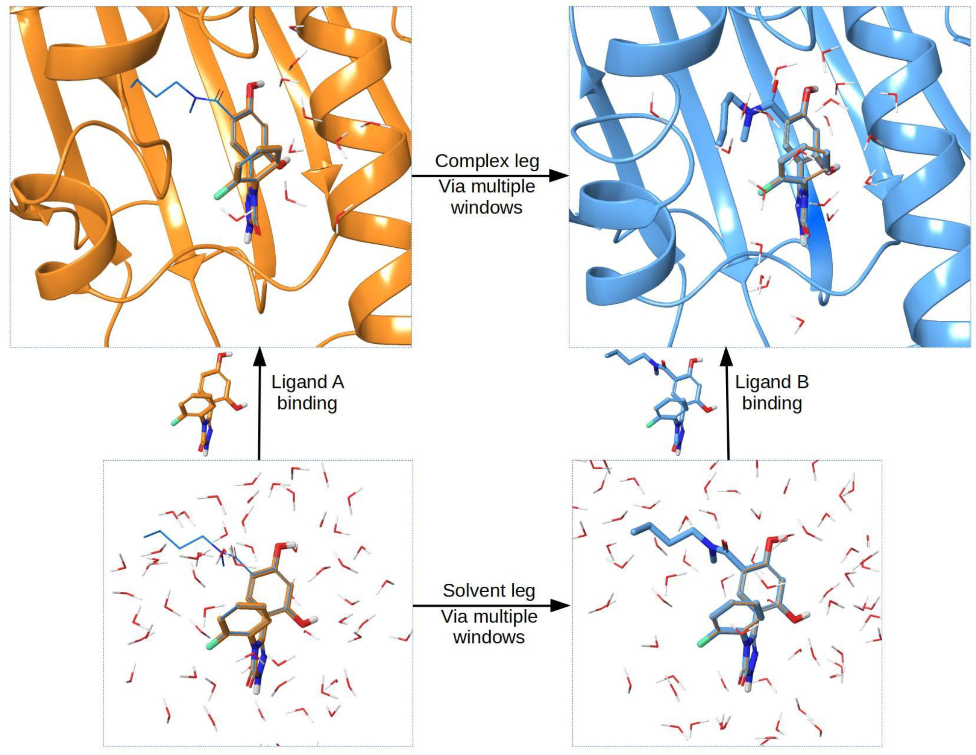
The thermodynamic cycle for FEP and MCFEP calculations. For relative binding FEP, the value of interest is calculating ΔΔG=ΔG_bindB - ΔG_bindA. Direct calculation of each vertical binding leg is impractical, instead FEP calculates an alchemical transformation from ligand A into ligand B. Based on the cycle, ΔΔG=ΔG_complex - ΔG_solvent, therefore the alchemical transformation is done for the two horizonal legs of ligand in complex and ligand in solvent, through multiple windows, known as complex and solvent legs in our tables. Ligand A is shown in orange, and ligand B is shown in blue, of which the orange region is also where the ligands have a structural core overlap. In our MCFEP, since the conformations of both the receptor and ligand are allowed to be different between the 2 ends, this is reflected in the figure. In actual simulation, even at both end windows, both ligands A and B exist, only that one ligand is 100% turned off in terms of interactions with all other molecules, but nonetheless exists and moves around for the purpose of calculating the ΔG of that window. Both ligands are shown in every window in figure to more accurately represent the FEP simulation.

Data Availability

Example tutorial runs, as well as the input files and output results for all cases presented in the paper are provided on the Github repository github.com/JL2021MD/MCFEP.

References

- 1.King E; Aitchison E; Li H; Luo R, Recent Developments in Free Energy Calculations for Drug Discovery. Front. Mol. Biosci 2021, 8. [DOI] [PMC free article] [PubMed] [Google Scholar]
- 2.Wang E; Sun H; Wang J; Wang Z; Liu H; Zhang JZH; Hou T, End-Point Binding Free Energy Calculation with MM/PBSA and MM/GBSA: Strategies and Applications in Drug Design. Chem. Rev. 2019, 119 (16), 9478–9508. [DOI] [PubMed] [Google Scholar]
- 3.Kuhn M; Firth-Clark S; Tosco P; Mey ASJS; Mackey M; Michel J, Assessment of Binding Affinity Via Alchemical Free-Energy Calculations. J. Chem. Inf. Model. 2020, 60 (6), 3120–3130. [DOI] [PubMed] [Google Scholar]
- 4.Abel R; Wang L; Harder ED; Berne BJ; Friesner RA, Advancing Drug Discovery through Enhanced Free Energy Calculations. Acc. Chem. Res. 2017, 50 (7), 1625–1632. [DOI] [PubMed] [Google Scholar]
- 5.Knight JL; Brooks CL III, Multisite Λ Dynamics for Simulated Structure–Activity Relationship Studies. J. Chem. Theory Comput. 2011, 7 (9), 2728–2739. [DOI] [PMC free article] [PubMed] [Google Scholar]
- 6.Jiang W, Accelerating Convergence of Free Energy Computations with Hamiltonian Simulated Annealing of Solvent (HSAS). J. Chem. Theory Comput 2019, 15 (4), 2179–2186. [DOI] [PubMed] [Google Scholar]
- 7.Ngo ST; Nguyen TH; Tung NT; Nam PC; Vu KB; Vu VV, Oversampling Free Energy Perturbation Simulation in Determination of the Ligand‐Binding Free Energy. J. Comput. Chem. 2020, 41 (7), 611–618. [DOI] [PubMed] [Google Scholar]
- 8.Jiang W; Roux B, Free Energy Perturbation Hamiltonian Replica-Exchange Molecular Dynamics (FEP/H-REMD) for Absolute Ligand Binding Free Energy Calculations. J. Chem. Theory Comput 2010, 6 (9), 2559–2565. [DOI] [PMC free article] [PubMed] [Google Scholar]
- 9.Jo S; Jiang W, A Generic Implementation of Replica Exchange with Solute Tempering (REST2) Algorithm in NAMD for Complex Biophysical Simulations. Comput. Phys. Commun. 2015, 197, 304–311. [Google Scholar]
- 10.Jiang W; Thirman J; Jo S; Roux B, Reduced Free Energy Perturbation/Hamiltonian Replica Exchange Molecular Dynamics Method with Unbiased Alchemical Thermodynamic Axis. J. Phys. Chem. 2018, 122 (41), 9435–9442. [DOI] [PMC free article] [PubMed] [Google Scholar]
- 11.Fratev F; Sirimulla S, An Improved Free Energy Perturbation FEP+ Sampling Protocol for Flexible Ligand-Binding Domains. Sci. Rep. 2019, 9 (1), 16829. [DOI] [PMC free article] [PubMed] [Google Scholar]
- 12.Wang L; Berne BJ; Friesner RA, On Achieving High Accuracy and Reliability in the Calculation of Relative Protein–Ligand Binding Affinities. Proc. Natl. Acad. Sci. 2012, 109 (6), 1937–1942. [DOI] [PMC free article] [PubMed] [Google Scholar]
- 13.Wang L; Wu Y; Deng Y; Kim B; Pierce L; Krilov G; Lupyan D; Robinson S; Dahlgren MK; Greenwood J; Romero DL; Masse C; Knight JL; Steinbrecher T; Beuming T; Damm W; Harder E; Sherman W; Brewer M; Wester R; Murcko M; Frye L; Farid R; Lin T; Mobley DL; Jorgensen WL; Berne BJ; Friesner RA; Abel R, Accurate and Reliable Prediction of Relative Ligand Binding Potency in Prospective Drug Discovery by Way of a Modern Free-Energy Calculation Protocol and Force Field. J. Am. Chem. Soc. 2015, 137 (7), 2695–2703. [DOI] [PubMed] [Google Scholar]
- 14.Deng Y; Roux B, Calculation of Standard Binding Free Energies: Aromatic Molecules in the T4 Lysozyme L99A Mutant. J. Chem. Theory Comput. 2006, 2 (5), 1255–1273. [DOI] [PubMed] [Google Scholar]
- 15.Morton A; Matthews BW, Specificity of Ligand Binding in a Buried Nonpolar Cavity of T4 Lysozyme: Linkage of Dynamics and Structural Plasticity. Biochemistry 1995, 34 (27), 8576–8588. [DOI] [PubMed] [Google Scholar]
- 16.Morton A; Baase WA; Matthews BW, Energetic Origins of Specificity of Ligand Binding in an Interior Nonpolar Cavity of T4 Lysozyme. Biochemistry 1995, 34 (27), 8564–8575. [DOI] [PubMed] [Google Scholar]
- 17.Stebbins CE; Russo AA; Schneider C; Rosen N; Hartl FU; Pavletich NP, Crystal Structure of an Hsp90–Geldanamycin Complex: Targeting of a Protein Chaperone by an Antitumor Agent. Cell 1997, 89 (2), 239–250. [DOI] [PubMed] [Google Scholar]
- 18.Amaral M; Kokh DB; Bomke J; Wegener A; Buchstaller HP; Eggenweiler HM; Matias P; Sirrenberg C; Wade RC; Frech M, Protein Conformational Flexibility Modulates Kinetics and Thermodynamics of Drug Binding. Nat. Commun. 2017, 8 (1), 2276. [DOI] [PMC free article] [PubMed] [Google Scholar]
- 19.Fajer M; Borrelli K; Abel R; Wang L, Quantitatively Accounting for Protein Reorganization in Computer-Aided Drug Design. J. Chem. Theory Comput. 2023, 19 (11), 3080–3090. [DOI] [PubMed] [Google Scholar]
- 20.Sergeeva AP; Katsamba PS; Liao J; Sampson JM; Bahna F; Mannepalli S; Morano NC; Shapiro L; Friesner RA; Honig B, Free Energy Perturbation Calculations of Mutation Effects on SARS-CoV-2 Rbd::Ace2 Binding Affinity. J. Mol. Biol. 2023, 435 (15), 168187. [DOI] [PMC free article] [PubMed] [Google Scholar]
- 21.Ha BH; Simpson MA; Koleske AJ; Boggon TJ, Structure of the ABL2/ARG Kinase in Complex with Dasatinib. Acta Crystallogr. Sect. F Struct. Biol. Cryst. Commun. 2015, 71 (4), 443–448. [DOI] [PMC free article] [PubMed] [Google Scholar]
- 22.Tokarski JS; Newitt JA; Chang CYJ; Cheng JD; Wittekind M; Kiefer SE; Kish K; Lee FYF; Borzillerri R; Lombardo LJ; Xie D; Zhang Y; Klei HE, The Structure of Dasatinib (BMS-354825) Bound to Activated ABL Kinase Domain Elucidates Its Inhibitory Activity against Imatinib-Resistant ABL Mutants. Cancer Res. 2006, 66 (11), 5790–5797. [DOI] [PubMed] [Google Scholar]
- 23.Salah E; Ugochukwu E; Barr AJ; von Delft F; Knapp S; Elkins JM, Crystal Structures of ABL-Related Gene (ABL2) in Complex with Imatinib, Tozasertib (VX-680), and a Type I Inhibitor of the Triazole Carbothioamide Class. J. Med. Chem. 2011, 54 (7), 2359–2367. [DOI] [PMC free article] [PubMed] [Google Scholar]
- 24.Young MA; Shah NP; Chao LH; Seeliger M; Milanov ZV; Biggs WH III; Treiber DK; Patel HK; Zarrinkar PP; Lockhart DJ; Sawyers CL; Kuriyan J, Structure of the Kinase Domain of an Imatinib-Resistant Abl Mutant in Complex with the Aurora Kinase Inhibitor VX-680. Cancer Res. 2006, 66 (2), 1007–1014. [DOI] [PubMed] [Google Scholar]
- 25.Xu W; Harrison SC; Eck MJ, Three-Dimensional Structure of the Tyrosine Kinase c-Src. Nature 1997, 385 (6617), 595–602. [DOI] [PubMed] [Google Scholar]
- 26.Hubbard SR; Wei L; Hendrickson WA, Crystal Structure of the Tyrosine Kinase Domain of the Human Insulin Receptor. Nature 1994, 372 (6508), 746–754. [DOI] [PubMed] [Google Scholar]
- 27.Rossari F; Minutolo F; Orciuolo E, Past, Present, and Future of Bcr-Abl Inhibitors: From Chemical Development to Clinical Efficacy. Journal of Hematology & Oncology 2018, 11 (1), 84. [DOI] [PMC free article] [PubMed] [Google Scholar]
- 28.Chen W; Cui D; Jerome SV; Michino M; Lenselink EB; Huggins DJ; Beautrait A; Vendome J; Abel R; Friesner RA; Wang L, Enhancing Hit Discovery in Virtual Screening through Absolute Protein–Ligand Binding Free-Energy Calculations. J. Chem. Inf. Model 2023, 63 (10), 3171–3185. [DOI] [PubMed] [Google Scholar]
- 29.Zhou T; Parillon L; Li F; Wang Y; Keats J; Lamore S; Xu Q; Shakespeare W; Dalgarno D; Zhu X, Crystal Structure of the T315I Mutant of Abl Kinase. Chem. Biol. Drug Des. 2007, 70 (3), 171–181. [DOI] [PubMed] [Google Scholar]
- 30.Wang L; Friesner RA; Berne BJ, Replica Exchange with Solute Scaling: A More Efficient Version of Replica Exchange with Solute Tempering (REST2). J. Phys. Chem. 2011, 115 (30), 9431–9438. [DOI] [PMC free article] [PubMed] [Google Scholar]
- 31.Carvalho Martins L; Cino EA; Ferreira RS, Pyautofep: An Automated Free Energy Perturbation Workflow for Gromacs Integrating Enhanced Sampling Methods. J. Chem. Theory Comput. 2021, 17 (7), 4262–4273. [DOI] [PubMed] [Google Scholar]
- 32.Cournia Z; Allen B; Sherman W, Relative Binding Free Energy Calculations in Drug Discovery: Recent Advances and Practical Considerations. J. Chem. Inf. Model. 2017, 57 (12), 2911–2937. [DOI] [PubMed] [Google Scholar]
- 33.Jacobson MP; Pincus DL; Rapp CS; Day TJF; Honig B; Shaw DE; Friesner RA, A Hierarchical Approach to All-Atom Protein Loop Prediction. Proteins: Struct., Funct., Bioinf 2004, 55 (2), 351–367. [DOI] [PubMed] [Google Scholar]
- 34.Sherman W; Day T; Jacobson MP; Friesner RA; Farid R, Novel Procedure for Modeling Ligand/Receptor Induced Fit Effects. J. Med. Chem. 2006, 49 (2), 534–553. [DOI] [PubMed] [Google Scholar]
- 35.Jumper J; Evans R; Pritzel A; Green T; Figurnov M; Ronneberger O; Tunyasuvunakool K; Bates R; Žídek A; Potapenko A; Bridgland A; Meyer C; Kohl SAA; Ballard AJ; Cowie A; Romera-Paredes B; Nikolov S; Jain R; Adler J; Back T; Petersen S; Reiman D; Clancy E; Zielinski M; Steinegger M; Pacholska M; Berghammer T; Bodenstein S; Silver D; Vinyals O; Senior AW; Kavukcuoglu K; Kohli P; Hassabis D, Highly Accurate Protein Structure Prediction with AlphaFold. Nature 2021, 596 (7873), 583–589. [DOI] [PMC free article] [PubMed] [Google Scholar]
- 36.Clark AJ; Gindin T; Zhang B; Wang L; Abel R; Murret CS; Xu F; Bao A; Lu NJ; Zhou T; Kwong PD; Shapiro L; Honig B; Friesner RA, Free Energy Perturbation Calculation of Relative Binding Free Energy between Broadly Neutralizing Antibodies and the Gp120 Glycoprotein of HIV-1. J. Mol. Biol. 2017, 429 (7), 930–947. [DOI] [PMC free article] [PubMed] [Google Scholar]
- 37.Clark AJ; Negron C; Hauser K; Sun M; Wang L; Abel R; Friesner RA, Relative Binding Affinity Prediction of Charge-Changing Sequence Mutations with FEP in Protein–Protein Interfaces. J. Mol. Biol. 2019, 431 (7), 1481–1493. [DOI] [PMC free article] [PubMed] [Google Scholar]
- 38.Steinbrecher T; Abel R; Clark A; Friesner R, Free Energy Perturbation Calculations of the Thermodynamics of Protein Side-Chain Mutations. J. Mol. Biol. 2017, 429 (7), 923–929. [DOI] [PubMed] [Google Scholar]
- 39.Roe DR; Cheatham TE III, PTRAJ and CPPTRAJ: Software for Processing and Analysis of Molecular Dynamics Trajectory Data. J. Chem. Theory Comput. 2013, 9 (7), 3084–3095. [DOI] [PubMed] [Google Scholar]
Associated Data
This section collects any data citations, data availability statements, or supplementary materials included in this article.
Supplementary Materials
Data Availability Statement