Cluster formation tracking of networked perturbed robotic systems via hierarchical fixed-time neural adaptive approach

Abstract

This paper investigates the fixed-time cluster formation tracking (CFT) problem for networked perturbed robotic systems (NPRSs) under directed graph information interaction, considering parametric uncertainties, external perturbations, and actuator input deadzone. To address this complex problem, a novel hierarchical fixed-time neural adaptive control algorithm is proposed based on a hierarchical fixed-time framework and a neural adaptive control strategy. The objective of this study is to achieve accurate CFT of NPRSs within a fixed time. Specifically, we design a distributed observer algorithm to estimate the states of the virtual leader within a fixed time accurately. By using these observers, a neural adaptive fixed-time controller is developed in the local control layer to ensure rapid and reliable system performance. Through the use of the Lyapunov argument, we derive sufficient conditions on the control parameters to guarantee the fixed-time stability of NPRSs. The theoretical results are eventually validated through numerical simulations, demonstrating the effectiveness and robustness of the proposed approach.

Introduction

Recently, there has been a growing interest in distributed cooperative control of multi-agent systems due to its various advantages over traditional centralized approaches. These advantages include increased flexibility, decentralization, and stronger robustness¹. As a result, this field has given rise to numerous research topics, such as consensus^2,3, tracking^4,5, distributed formation control^6,7, containment⁸, and flocking⁹. However, most existing literature in this area focuses on systems with single- or double-integrator dynamics and Lipschitz-type dynamics. Although these dynamics are suitable for many applications, the use of such models may not be sufficiently rigorous for networked robotic systems, which are typical examples of multi-agent systems. Instead, employing Euler–Lagrange dynamics provides a more accurate representation of real-world robotic systems and their interactions. This distinction highlights the need for more specialized and precise control strategies of networked robotic systems.

Therefore, many researchers have been directing their effort toward the collaborative control of networked robotic systems with Euler–Lagrange dynamics^10–12. However, the existence of actuator input deadzone, parametric uncertainties, and external perturbations is inevitable in networked perturbed robotic systems (NPRSs). These deadzone characteristics often arise in practical robotic systems due to factors such as friction, backlash, and mechanical wear, which introduce nonlinearities and can significantly impair system performance^13,14. In addition, NPRSs exhibit inherent characteristics, such as nonlinearity, susceptibility to uncertainties, and inter-joint couplings, further complicating their analysis and control. To address these difficulties, several control algorithms have been developed, including adaptive control¹⁵, fuzzy control¹⁶, robust control¹⁷, and sliding mode control¹⁸. In particular, sliding mode control has gained significant attention due to its potential for achieving finite convergence^19–21/fixed-time convergence^22–27and robustness in the presence of uncertainties. While finite-time stability ensures convergence within a time frame that depends on the system’s initial conditions, fixed-time stability guarantees convergence regardless of these initial conditions. This key difference enhances system predictability and performance reliability, making fixed-time stability particularly useful in time-critical applications. Significantly, under the framework of finite-time control for switched nonlinear systems with multiple objective constraints, an adaptive finite-time controller based on a multi-dimensional Taylor network is proposed, ensuring constraint compliance and avoiding singularity²¹. Polyakov et al. have utilized theorems on Lyapunov functions for fixed-time stability analysis to design nonlinear control laws for the robust stabilization of a chain of integrators²⁴. Based on the framework of input-output linearization, the challenge of fixed-time stabilization for nonlinear systems with a full relative degree has been addressed by developing homogeneous feedback laws²⁷. However, achieving fixed-time stability for NPRSs remains an open problem.

Moreover, constructing appropriate equivalent terms to approximate the lumped uncertainty terms of a system is particularly challenging. These uncertainty terms include actuator input deadzone, external perturbations, and parametric uncertainties. Recently, interest in utilizing radial basis function (RBF) neural networks for approximating unknown nonlinear functions has been increasing^28,29. In the context of multi-agent systems, the neural network approach presumes that the uncertainties within the system can be accurately approximated by a neural network with adequate capacity and training data. It also presupposes that the dynamics of the multi-agent system can be accurately represented by the neural network to capture the nonlinear characteristics of these uncertainties. Under the neural network-based control strategy, the challenge of fixed-time formation control in nonlinear multi-agent systems has been addressed³⁰. Within the framework of backstepping and utilizing predefined-time stability, the predefined-time adaptive neural tracking control problem for nonlinear multi-agent systems is investigated in³¹. Hierarchical control strategies, in particular, offer considerable advantages for managing multi-agent systems by enhancing robustness and scalability^32,33. By breaking down a global problem into smaller sub-problems, hierarchical framework reduce computational complexity and enhance overall system stability and coordination. Building on this interest, we propose a novel hierarchical fixed-time neural adaptive (HFNA) control algorithm that combines the fixed-time algorithm that uses a hierarchical framework with an RBF neural network. This innovative approach aims to enhance steady-state performance compared with that of conventional methods.

Meanwhile, existing research on cooperative control has focused on cooperative tracking²⁵ and formation tracking^34–38, where all robots converge to a single stable state or formation. Specifically, Cheng et al. have investigated single time-varying formation control for heterogeneous multi-agent systems, addressing actuator faults, uncertainties, and perturbations³⁴. Under an adaptive fuzzy control approach combined with a periodic adaptive event-triggered control scheme, single fixed-time formation control for multi-agent systems facing actuator failures is achieved³⁵. Based on a low-complexity control framework ensuring prescribed performance, single formation tracking for networked underactuated surface vessels in a fully quantized environment has been addressed in³⁸. However, these results are not directly applicable to scenarios wherein networked robotic systems are required to perform multiple tasks simultaneously. This motivation has led to research on group consensus³⁹ and multi-tracking⁴⁰. However, most of the aforementioned studies primarily address state coordination problems in networked robotic systems. By contrast, the current study focuses on the cluster formation tracking (CFT) problem, which involves coordinating the output of subnetworks in an NPRS to form multiple desired formations in local coordinates. Each chosen reference point follows a predefined trajectory in global coordinates while maintaining the formation. In the CFT control task scenario of NPRSs, as shown in Fig. 1, it becomes indispensable to study the fixed-time problem in CFT of NPRSs. This is particularly important when considering actuator input deadzone, external perturbations, and parametric uncertainties, as it addresses a fundamental challenge in the control of networked robotic systems.

Fig. 1.

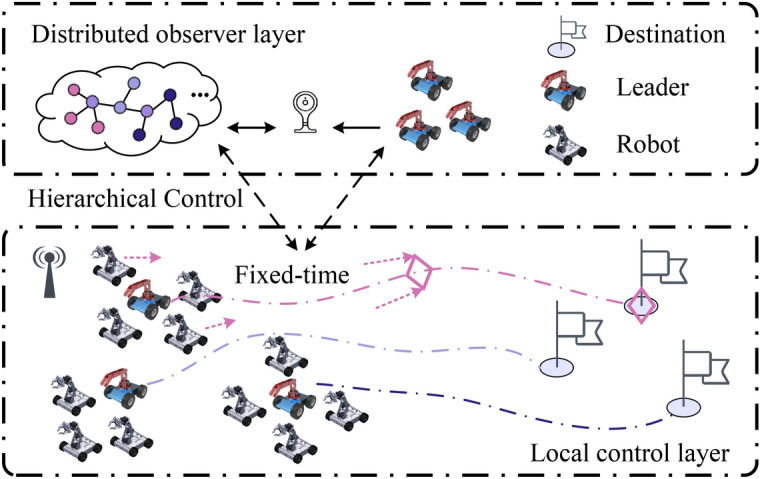
Cluster formation tracking control scenario of NPRS.

Motivated by the aforementioned discussions, this paper introduces the HFNA control algorithm, specifically crafted to address the intricate challenges of fixed-time CFT in NPRSs. By focusing on key issues such as parametric uncertainties, external perturbations, and actuator input deadzone, the HFNA algorithm aims to enhance the robustness and effectiveness of multi-robot coordination. The following are the main contributions of this paper.

• In contrast with prior research on the finite-time stability of NPRSs, where error states typically reach the origin within a finite time that is dependent on the initial condition^19–21, we propose a novel HFNA control algorithm that achieves fixed-time stability independent of the initial condition, ensuring a controllable convergence time, which enhances the predictability and reliability of the system’s performance.

• The proposed HFNA control algorithm provides a comprehensive framework for fixed-time CFT under directed graphs, addressing key challenges in existing studies^34,36,38,41 by systematically managing parametric uncertainties, external perturbations, and actuator input deadzone.

• Different from the conventional fixed-time control algorithms for networked robotic systems^26,27, the HFNA control algorithm effectively addresses lumped uncertainty terms while exhibiting minimal chattering by utilizing RBF neural networks to approximate the lumped uncertainty.

The remaining sections are organized in the following sequence. Section Preliminaries provides preliminaries on graph theory, stability theory, neural networks, function approximation, systems, and problems. Section Major results describes the designed HFNA control algorithm with the corresponding convergence analysis. Section Simulations presents the simulation results. Eventually, a concise summary of conclusions is provided in Section Conclusion.

Notations: Let ${\mathbb{R}}^d$ be the d-dimensional Euclidean space. ${\mathbb{R}}^{d\times d}$ represents a $d\times d$ real matrix. $\otimes$ denotes the Kronecker product. ${\mathbf{1}}_d$ refers to a d-dimensional vector with elements equal to 1. The symbols $max\{·\}$ and $min\{·\}$ denote maximum and minimum magnitudes, respectively. ${∥·∥}_p$ represents the p-norm. Moreover, the column vectors $a·b=\mathrm{col}(a_1{b}_1,a_1{b}_1,\dots ,a_1{b}_1)$, $\forall a=\mathrm{col}(a_1,a_1,\dots ,a_d)\in {\mathbb{R}}^d$, and $b=\mathrm{col}(b_1,b_2,\dots ,b_n)\in {\mathbb{R}}^d$. For the provided $\varsigma =\text{col}({\varsigma }_1,{\varsigma }_2,\dots ,{\varsigma }_N)$ and $\rho >0$, it follows that $\text{sig}{(\varsigma )}^{\rho }=\text{col}(\text{sgn}({\varsigma }_1)|{\varsigma }_1{|}^{\rho },\text{sgn}({\varsigma }_2)|{\varsigma }_2{|}^{\rho },\dots ,\text{sgn}({\varsigma }_N)|{\varsigma }_N{|}^{\rho })$ and $\text{diag}(\varsigma )=\text{diag}({\varsigma }_1,{\varsigma }_2,\dots ,{\varsigma }_N)$.

Preliminaries

Graph theory

In this paper, we consider a NPRS comprising N robots. The communication topology in NPRS is crucial, as it defines how robots exchange information. This topology forms the foundation for both the formulation of the control problem and the control design. To represent these interactions, we introduce a directed graph $\mathcal{G}=\left\{\mathcal{V},\mathcal{E},\mathcal{A}\right\}$, where $\mathcal{V}$ denotes the set of vertices representing the robots, $\mathcal{E}\subset \mathcal{V}\times \mathcal{V}$ is the edge set, and $\mathcal{A}=\left[a_{\mathit{ij}}\right]\in {\mathbb{R}}^{N\times N}$ is the adjacency matrix. $e_{\mathit{ij}}\in \mathcal{E}$ represents the direct information flow from robot j to robot i. More precisely, we establish $a_{\mathit{ij}}>0$ to represent cooperation between robot i and robot j; $a_{\mathit{ij}}<0$ to indicate competition; otherwise, $a_{\mathit{ij}}=0$ signifies no interaction. In addition, the directed graph $\mathcal{G}$ is acyclic, i.e., $a_{\mathit{ii}}=0$. ${\mathcal{N}}_i=\left\{j\in \mathcal{V}\left|,e_{\mathit{ij}}\in \mathcal{E}\right)\right\}$ denotes the neighbor set of robot i. The Laplacian matrix $\mathcal{L}=\left[l_{\mathit{ij}}\right]\in {\mathbb{R}}^{N\times N}$ of $\mathcal{G}$ is defined such that $l_{\mathit{ij}}=-a_{\mathit{ij}}$ and $l_{\mathit{ii}}={\sum }_{j\in {\mathcal{N}}_i}{a}_{\mathit{ij}}$ for $i\ne j\in \mathcal{V}$. Moreover, $\mathcal{G}$ can be partitioned into $\mathcal{K}$ subnetworks denoted by ${\mathcal{G}}_k=\left\{{\mathcal{V}}_k,{\mathcal{E}}_k,{\mathcal{A}}_k\right\}$ with each comprising $n_k$ robots, where $k\in \{1,2,\dots ,\mathcal{K}\}$, ${\mathcal{V}}_k\cap {\mathcal{V}}_m=\mathrm{\varnothing }$ for all $k\ne m\in \{1,2,\dots ,\mathcal{K}\}$, ${\sum }_{k=1}^{\mathcal{K}}{\mathcal{V}}_k=\mathcal{V}$ and ${\sum }_{k=1}^{\mathcal{K}}{n}_k=N$. Specifically, ${\mathcal{V}}_k=\{1+{\sum }_{i=1}^k{n}_{i-1},\dots ,{\sum }_{i=1}^k{n}_i\}$ is utilized to describe the nodes of the kth subnetwork with $n_0=0$. Besides, each subnetwork has $\mathcal{K}$ corresponding virtual leaders. The interactions among robots and virtual leaders are captured by the diagonal weighted matrix $\mathcal{B}=\text{diag}\left(b_1,b_2,\dots ,b_N\right)$. When the ith robot is able to receive information from its virtual leader, we have $b_i>0$; otherwise, $b_i=0$. Let ${\mathcal{B}}_k$ represent the diagonal weighted matrix associated with ${\mathcal{G}}_k$. Then, $\mathcal{B}=\text{diag}\left({\mathcal{B}}_1,{\mathcal{B}}_2,\dots ,{\mathcal{B}}_{\mathcal{K}}\right)$.

Assumption 1

The directed graph $\mathcal{G}$ can be partitioned into a sequence $\{{\mathcal{V}}_1,{\mathcal{V}}_2,\dots ,{\mathcal{V}}_{\mathcal{K}}\}$ such that no cycles occur within this partition. Within each subnetwork, the information of the virtual leader is accessible to all individuals globally.

Assumption 2

For any given $i\in {\mathcal{V}}_k$ and $k\ne m\in \{1,2,\dots ,\mathcal{K}\}$, the sum of the connection weights between robot i and the robots in subnetwork m is equal to zero to ensure that the interaction in subnetwork m is balanced in terms of its influence on NPRS, i.e., ${\sum }_{j={\varsigma }_k}^k{l}_{\mathit{ij}}=0$, where ${\varsigma }_k=1+{\sum }_{i=1}^k{n}_{i-1}$ and ${\tilde{\varsigma }}_k={\sum }_{i=1}^k{n}_i$.

Remark 1

Unlike previous work on single formation^34,36–38, which may not explicitly enforce an acyclic structure within a partition, Assumption 1 ensures that information from the virtual leader is accessible to all individuals globally within each subnetwork. Assumption 2 means that the sum of connection weights between robot i and robots in subnetwork m equals zero, not requiring the sum of weights within each subnetwork to be zero. Negative edge weights represent inhibitory constraints on interactions among robots. They are included to illustrate scenarios where interactions within a subnetwork offset each other, resulting in a neutral effect on a specific robot’s behavior.

Finite- and fixed-time stability

Imagine a differential system in the following manner:

$$\begin{array}{c}\hfill \dot{z}=f(z,t),z(0)=z_0,\end{array}$$ 1

where $z\in {\mathbb{R}}^d$ represents the system state, $f(·)$ denotes a nonlinear function, and $z_0\in {\mathbb{R}}^d$ is the initial state.

Definition 1

¹⁰ System (1) is considered to exhibit finite-time stability if it satisfies the conditions of Lyapunov stability and there exists a settling time function $\mathcal{T}(z_0)$ such that $\left|{\mathrm{\Phi }}_z(t,z_0)\right|=0$ for $t\in [\mathcal{T}(z_0),+\infty ]$. Unlike autonomous systems, the Lyapunov function V(z, t) and the stability conditions explicitly depend on time, incorporating additional terms to reflect this time dependency.

Definition 2

²² System (1) is characterized as fixed-time stability if it satisfies the conditions of finite-time stability and a settling time function $\mathcal{T}(z_0)$ that is bounded by a constant exists. In simpler terms, there exists a maximum settling time $\mathcal{T}max>0$ such that $f(z(t))=0$, $\forall t\ge \mathcal{T}max$ and $\forall \mathcal{T}(z_0)\le \mathcal{T}max$, $z_0\in {\mathbb{R}}^d$.

Lemma 1

²² Given a system described as system (1), if a continuous positive-definite function V(z) satisfies the condition

$$\begin{array}{c}\hfill \frac{\partial V}{\partial z}f(z,t)\le -\sigma V^{\frac{{\ell }_1}{{\gamma }_1}}(z)-\eta V^{\frac{{\ell }_2}{{\gamma }_2}}(z),\end{array}$$

where $\sigma >0$, $\eta >0$, ${\ell }_1$, ${\gamma }_1$, ${\ell }_2$, and ${\gamma }_2$ are positive odd integers that satisfy ${\ell }_1>{\gamma }_1$ and ${\ell }_2<{\gamma }_2$. In such case, the origin of the system is a globally fixed-time stable equilibrium, with the settling time function $\mathcal{T}$ limited by

$$\begin{array}{c}\hfill \mathcal{T}\le {\mathcal{T}}_{max}=\frac{1}{\sigma }\frac{{\gamma }_1}{{\ell }_1-{\gamma }_1}+\frac{1}{\eta }\frac{{\gamma }_2}{{\gamma }_2-{\ell }_2}.\end{array}$$

Furthermore, if $\theta \stackrel{\mathrm{\Delta }}{=}[{\gamma }_2({\ell }_1-{\gamma }_1)]/[{\gamma }_1({\gamma }_2-{\ell }_2)]\le 1$, we can obtain a less conservative estimate of the time function$\mathcal{T}$as

$$\begin{array}{c}\hfill \mathcal{T}\le {\mathcal{T}}_{max}=\frac{{\gamma }_2}{{\gamma }_2-{\ell }_2}\left(\frac{1}{\sqrt{\sigma \eta }}{tan}^{-1}\sqrt{\frac{\sigma }{\eta }}+\frac{1}{\sigma \theta }\right).\end{array}$$

Neural network principle

As depicted in Fig. 2, the RBF neural network is typically characterized by the neural structure that consists of an input layer, a hidden layer, and an output layer. The primary purposes of these layers are as follows: the input layer is responsible for receiving external information, the hidden layer performs nonlinear transformations, and the output layer provides the final output information. RBF neural networks are a suitable choice in this scenario due to their capability to estimate unknown nonlinear functions effectively²³. Therefore, we employ RBF neural networks to estimate a nonlinear function $g(·):{\mathbb{R}}^b\to {\mathbb{R}}^d$.

Fig. 2.

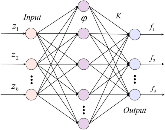
RBF neural network.

The RBF neural network approximates the function g(z) as follows:

$$\begin{array}{c}\hfill g(z)\approx \widehat{g}(z)=K^T\phi (z)+\epsilon ,\end{array}$$

where the weight matrix $K\in {\mathbb{R}}^{m\times d}$ consists of the weights of m neurons, and the input data vector is denoted as $z\in {\mathbb{R}}^b$. The approximation error of a RBF neural network is represented by $\epsilon \in {\mathbb{R}}^d$. To derive this, consider the basis function $\phi ={\left[{\phi }_j(z)\right]}_{m\times 1}\in {\mathbb{R}}^m$, defined as:

$$\begin{array}{c}\hfill {\phi }_j(z)=exp\left[-\frac{1}{2{\iota }_j}∥z-{\rho }_j∥\right],\forall j\in \{1,2,\dots ,m\},\end{array}$$

where ${\rho }_j\in {\mathbb{R}}^b$ is the center of the jth neuron and ${\iota }_j$ represents the width of this neuron. A practical rule for choosing the width ${\iota }_j$ for each neuron based on the distance between the centers can be expressed as:

$$\begin{array}{c}\hfill {\iota }_j=\frac{1}{m}\sum _{k=1}^m\Vert {\rho }_j-{\rho }_k\Vert .\end{array}$$

The width of a neuron remains a positive constant when the neuron is a hidden neuron. This ensures that each neuron’s receptive field overlaps with its neighbors, providing smooth transitions and improved approximation capabilities.

The RBF network’s output is a linear combination of these basis functions weighted by the matrix K. This can be expressed as:

$$\begin{array}{c}\hfill \widehat{g}(z)=\sum _{j=1}^m{K}_j{\phi }_j(z),\end{array}$$

where $K_j\in {\mathbb{R}}^b$ is the weight vector associated with the jth neuron.

By minimizing the approximation error $\epsilon$ between the actual function g(z) and the observed function $\widehat{g}(z)$, the weights K are adjusted to ensure that the RBF neural network can approximate g(z) as accurately as possible. This is typically done through a learning algorithm such as gradient descent.

System statement

In this scenario, we examine an example that involves a NPRS that consists of N robots. The dynamics and kinematics of the ith robot can be represented by

$$\begin{array}{c}\hfill H_i(q_i){\ddot{q}}_i+C_i(q_i,{\dot{q}}_i){\dot{q}}_i+G_i(q_i)+d_i(t)=\psi ({\tau }_i),\end{array}$$ 2

where the position, velocity, and acceleration vectors of the robot are denoted as $q_i,{\dot{q}}_i$, and ${\ddot{q}}_i\in {\mathbb{R}}^d$, respectively. $H_i(q_i)\in {\mathbb{R}}^{d\times d}$ represents the robotic inertia matrix. $C_i(q_i,{\dot{q}}_i)\in {\mathbb{R}}^{d\times d}$ denotes the Coriolis centrifugal matrix. $G_i(q_i)$ represents the gravitational torque. $d_i(t)$ represents external perturbations that affect the robot. ${\tau }_i\in {\mathbb{R}}^d$ includes the calculated control signals. $\psi ({\tau }_i)\in {\mathbb{R}}^d$ is the deadzone function of the input torque, i.e.,

$$\begin{array}{c}\hfill \psi ({\tau }_i)=\left\{\begin{array}{c}{u}_h({\tau }_i-{\delta }_h{\mathbf{1}}_d),∥{\tau }_i∥\ge {\delta }_h,\hfill \\ 0,{\delta }_l<∥{\tau }_i∥<{\delta }_h,\hfill \\ u_l({\tau }_i-{\delta }_l{\mathbf{1}}_d),∥{\tau }_i∥\le {\delta }_l,\hfill \end{array}\right)\end{array}$$

where the constants ${\delta }_l$ and ${\delta }_h$ represent the bounds of the deadzone. In addition, $u_l(·)$ and $u_h(·)$ refer to the uncertain deadzone functions. Furthermore, to account for parametric uncertainties, the unknown $\psi ({\tau }_i)$ can be decomposed into two components: $\psi ({\tau }_i)\stackrel{\mathrm{\Delta }}{=}{\tau }_i-\mathrm{\Delta }{\tau }_i$, where $\mathrm{\Delta }{\tau }_i$ denotes an unknown continuous error function. Accounting for the presence of parametric uncertainties, the dynamical terms take the form of

$$\begin{array}{cc}& H_i(q_i)=H_{i0}(q_i)+\mathrm{\Delta }{H}_i(q_i),\hfill \\ \hfill & C_i(q_i,{\dot{q}}_i)=C_{i0}(q_i,{\dot{q}}_i)+\mathrm{\Delta }{C}_i(q_i,{\dot{q}}_i),\hfill \\ \hfill & G_i(q_i)=G_{i0}(q_i)+\mathrm{\Delta }{G}_i(q_i),\hfill \end{array}$$

where the terms $H_{i0}(q_i)$, $C_{i0}(q_i,{\dot{q}}_i)$, and $G_{i0}(q_i)$ are known and provided by the user, directly usable for control design. By contrast, $\mathrm{\Delta }{H}_i(q_i)$, $\mathrm{\Delta }{C}_i(q_i,{\dot{q}}_i)$, and $\mathrm{\Delta }{G}_i(q_i)$ are uncertain terms that arise due to inevitable measurement errors in practical applications. Consequently, System (2) can be reformulated as follows:

$$\begin{array}{c}\hfill H_{i0}(q_i){\ddot{q}}_i+C_{i0}(q_i,{\dot{q}}_i){\dot{q}}_i+G_{i0}(q_i)={\tau }_i+F_i(t),\end{array}$$ 3

where the consideration of lumped uncertainty terms $F_i(t)=-\mathrm{\Delta }{H}_i(q_i){\ddot{q}}_i-\mathrm{\Delta }{C}_i(q_i,{\dot{q}}_i){\dot{q}}_i-\mathrm{\Delta }{G}_i(q_i)-d_i(t)-\mathrm{\Delta }{\tau }_i$$F_i(t)=-\mathrm{\Delta }{H}_i(q_i){\ddot{q}}_i-\mathrm{\Delta }{C}_i(q_i,{\dot{q}}_i){\dot{q}}_i-\mathrm{\Delta }{G}_i(q_i)-d_i(t)-\mathrm{\Delta }{\tau }_i$ encompasses the effects of parametric perturbations $\mathrm{\Delta }{H}_i(q_i)$, $\mathrm{\Delta }{C}_i(q_i,{\dot{q}}_i)$, and $\mathrm{\Delta }{G}_i(q_i)$, as well as external disturbances $d_i(t)$, and actuator input deadzone $\mathrm{\Delta }{\tau }_i$. Utilizing RBF neural networks, $F_i(t)$ can be represented as follows:

$$\begin{array}{c}\hfill F_i(t)=K_i^T{\phi }_i(z_i)+{\epsilon }_i,\end{array}$$ 4

where $K_i\in {\mathbb{R}}^{m\times d}$ represents the weight matrix associated with m neurons. The input vector is denoted as $z_i\in {\mathbb{R}}^b$. Furthermore, ${\epsilon }_i\in {\mathbb{R}}^d$ represents the neural network approximation error, assumed to be bounded, i.e., $∥{\epsilon }_i∥\le {\varpi }_i$, ${\varpi }_i$ is a positive constant. In this case, ${\phi }_i(z_i)={\left[{\phi }_{\mathit{ij}}(z_i)\right]}_{m\times 1}$ represents the Gaussian function associated with the RBF neural network, and

$$\begin{array}{c}\hfill {\phi }_{\mathit{ij}}(z_i)=exp\left[-\frac{1}{2{\iota }_j}∥z_i-{\rho }_j∥\right],\forall j\in \{1,2,\dots ,m\}.\end{array}$$

${\rho }_j\in {\mathbb{R}}^b$ represents the center of the jth neuron, while ${\iota }_j$ denotes the width of the same neuron.

Subsequently, NPRS (3) can be reformulated as follows:

$$\begin{array}{c}\hfill H_{i0}(q_i){\ddot{q}}_i+C_{i0}(q_i,{\dot{q}}_i){\dot{q}}_i+G_{i0}(q_i)={\tau }_i+K_i^T{\phi }_i(z_i)+{\epsilon }_i.\end{array}$$ 5

Notably, the following salient properties distinctly characterize the model of NPRS (2).

Property 1

The inertia matrix $H_i(q_i)$ is known to possess the properties of symmetry and positive definiteness.

Property 2

The matrix ${\dot{H}}_i(q_i)-2C_i(q_i,{\dot{q}}_i)$ exhibits the property of skew-symmetry.

Furthermore, with regard to the kth subnetwork, the dynamics of the virtual leader’s trajectory are given by

$$\begin{array}{c}\hfill \left\{\begin{array}{c}{\dot{x}}_{0,k}=v_{0,k},\hfill \\ {\dot{v}}_{0,k}=a_{0,k},\hfill \end{array}\right)\end{array}$$

where $x_{0,k},v_{0,k}$, and $a_{0,k}\in {\mathbb{R}}^d$ represent the position, velocity, and acceleration vectors of the kth virtual leader, respectively, $\forall k\in \mathcal{K}$. Here, we present a justifiable assumption that concerns the virtual leaders.

Assumption 3

Acceleration $a_{0,k}$ is bounded by a nonnegative constant ${\delta }_{0,k}$, such that $∥a_{0,k}∥\le {\delta }_{0,k}$.

Remark 2

RBF networks are particularly advantageous for our application due to their universal approximation capabilities, enabling accurate approximation of continuous functions with sufficient neurons in the hidden layer. This makes them effective for modeling and compensating for system nonlinearities and uncertainties. Additionally, RBF networks are well-suited for capturing complex, nonlinear disturbances that are challenging for observer techniques. Their effectiveness in similar applications has been demonstrated in previous studies^23,28,29, further supporting our choice.

Remark 3

The NPRS (2) can be extended to form a mobile manipulator when integrated with a mobile platform. This system comprises a nonholonomic mobile base and a holonomic manipulator. Specifically, consider a two-wheel-driven mobile platform operating under non-slip conditions. When factoring in parametric uncertainties, the system’s dynamics can be written as:

$$\begin{array}{c}\hfill \left\{\begin{array}{c}{H}_{i022}{\ddot{q}}_{\mathit{ia}}+C_{i022}{\dot{q}}_{\mathit{ia}}+G_{i0a}+f_{\mathit{ia}}={\tau }_{\mathit{ia}},\hfill \\ H_{i011}{\ddot{q}}_{\mathit{ib}}+C_{i011}{\dot{q}}_{\mathit{ib}}+G_{i0b}+U_{\mathit{ib}}=B_{\mathit{ib}}{\tau }_{\mathit{ib}}-A_{\mathit{ib}}^{\mathrm{T}}{\vartheta }_i,\hfill \end{array}\right)\end{array}$$

where $q_i=\text{col}(q_{\mathit{ia}},q_{\mathit{ib}})$, ${\tau }_i=\text{col}({\tau }_{\mathit{ia}},{\tau }_{\mathit{ib}})$, $d_i=\text{col}(d_{\mathit{ia}},d_{\mathit{ib}})$, $C_i=[C_{i11},C_{i12};C_{i21},C_{i22}]$, $f_{\mathit{ia}}=\mathrm{\Delta }{H}_{i22}{\ddot{q}}_{\mathit{ia}}+\mathrm{\Delta }{C}_{i22}{\dot{q}}_{\mathit{ia}}+\mathrm{\Delta }{G}_{\mathit{ia}}+d_{\mathit{ia}}+H_{i21}{\ddot{q}}_{\mathit{ib}}+C_{i21}{\dot{q}}_{\mathit{ib}}$, $U_{\mathit{ib}}=\mathrm{\Delta }{H}_{i11}{\ddot{q}}_{\mathit{ib}}+\mathrm{\Delta }{C}_{i11}{\dot{q}}_{\mathit{ib}}+\mathrm{\Delta }{G}_{\mathit{ib}}+d_{\mathit{ib}}+H_{i12}{\ddot{q}}_{\mathit{ia}}+C_{i12}{\dot{q}}_{\mathit{ia}}$ with $A_{\mathit{ib}}$ denoting the constraint matrix, $B_{\mathit{ib}}$ as the transformation matrix, and ${\vartheta }_i$ representing the Lagrange multiplier.

Problem formulation

The primary focus is to investigate the fixed-time CFT problem of NPRSs described below. The following form of problem definition is provided using the principle of fixed-time stability.

Definition 3

The achievement of the fixed-time CFT problem of NPRSs is determined by the existence of a settling time ${\mathcal{T}}_{max}$, which remains independent of the initial condition, such that

$$\begin{array}{c}\hfill \left\{\begin{array}{c}{lim}_{t\to {\mathcal{T}}_{max}}∥q_i(t)-r_i-x_{0,k}(t)∥=0,\hfill \\ {lim}_{t\to {\mathcal{T}}_{max}}∥{\dot{q}}_i(t)-v_{0,k}(t)∥=0,\hfill \\ ∥q_i(t)-r_i-x_{0,k}(t)∥=0,\forall t\in [{\mathcal{T}}_{max},\infty ),\hfill \\ ∥{\dot{q}}_i(t)-v_{0,k}(t)∥=0,\forall t\in [{\mathcal{T}}_{max},\infty ),\hfill \end{array}\right)\end{array}$$

where $q_i(t)$ and ${\dot{q}}_i(t)\in {\mathbb{R}}^d$ are the robot’s position and velocity defined in formula (2), and $r_i\in {\mathbb{R}}^d$ denotes the ith robot’s formation offset.

Remark 4

In the practical application of CFT for the NPRS, uncertain factors, such as device precision, actuator limitations, and variations in operating conditions, inevitably result in negative effects, such as reduced control accuracy and difficulties in determining the time when the system becomes stable. Consequently, considering actuator input deadzone, parametric uncertainties, and external perturbations, becomes of paramount importance.

Major results

This section introduces a new HFNA control algorithm tailored to address the CFT problem for NPRSs while ensuring fixed-time convergence capability. Additionally, the effectiveness of the algorithm is verified by the following stability analysis.

HFNA control algorithm

In this subsection, we present the HFNA control algorithm for NPRSs. Before proceeding further, we define ${\widehat{e}}_i=q_i-r_i-{\widehat{x}}_i$, ${\dot{\widehat{e}}}_i={\dot{q}}_i-{\widehat{v}}_i$, and ${\ddot{\widehat{e}}}_i={\ddot{q}}_i-{\widehat{a}}_i$, where ${\widehat{x}}_i$, ${\widehat{v}}_i$, and ${\widehat{a}}_i$ are the observations of $q_i$, ${\dot{q}}_i$, and ${\ddot{q}}_i$, respectively. Moreover, we design a fixed-time sliding vector as follows:

$$\begin{array}{c}\hfill {\widehat{s}}_i={\widehat{e}}_i+{\left({ħ}_i^{-1}·{\dot{\widehat{e}}}_i\right)}^{n_4/m_4},{ħ}_i={\sigma }_0{\widehat{e}}_i^{m_3/n_3-m_4/n_4}+{\eta }_0{\mathbf{1}}_d,\end{array}$$

where ${\widehat{s}}_i\in {\mathbb{R}}^d$, $m_3$, $n_3$, $m_4$, and $n_4$ are positive odd integers that satisfy $m_3>n_3$, $m_4<n_4<2m_4$, and $m_3/n_3-m_4/n_4>0$. ${\sigma }_0$ and ${\eta }_0$ are positive constants.

In this manner, let ${\widehat{\xi }}_i=\mathrm{col}({\widehat{x}}_i,{\widehat{v}}_i,{\widehat{a}}_i)\in {\mathbb{R}}^{3d}$ and ${\gamma }_{0,k}=\mathrm{col}(x_{0,k},v_{0,k},a_{0,k})\in {\mathbb{R}}^{3d}$. In the presence of actuator input deadzone, parametric uncertainties and external perturbations, the HFNA control algorithm is formulated in the following manner:

$$\begin{array}{c}\hfill \left\{\begin{array}{c}\begin{array}{cc}\hfill {\tau }_i& ={\tau }_{i,1}+{\tau }_{i,2}\hfill \\ \hfill {\tau }_{i,1}& =C_{i0}{\dot{q}}_i+G_{i0}-{\widehat{K}}_i^T{\phi }_i-{\widehat{\varpi }}_i-{\beta }_i\mathrm{sig}({\widehat{s}}_i)\hfill \\ \hfill {\tau }_{i,2}& =H_{i0}{\widehat{a}}_i-H_{i0}{\dot{q}}_i-H_{i0}({\mathrm{\Gamma }}_i·{\dot{\widehat{e}}}_i^2·{ħ}_i^{-1})\hfill \\ \hfill & -\frac{m_4}{n_4}{H}_{i0}{ħ}_i·{({ħ}_i^{-1}·{\dot{\widehat{e}}}_i)}^{\frac{m_4-n_4}{m_4}}·({\dot{\widehat{e}}}_i+{\delta }_i)\hfill \\ \hfill {\dot{\widehat{K}}}_i& ={\alpha }_1{\phi }_i{\widehat{s}}_i^T,{\dot{\widehat{\varpi }}}_i={\alpha }_2∥{\widehat{s}}_i∥,\hfill \end{array}\hfill \end{array}\right)\end{array}$$ 6

$$\begin{array}{c}\hfill \left\{\begin{array}{c}\begin{array}{cc}\hfill {\dot{\widehat{\xi }}}_i=& {\left(\sum _{j\in {\mathcal{N}}_i}{a}_{\mathit{ij}}+b_i\right)}^{-1}\left[\sum _{j\in {\mathcal{N}}_i},a_{\mathit{ij}}{\dot{\widehat{\xi }}}_j,+,b_i,{\dot{\gamma }}_{0,k}\right)\hfill \\ \hfill & -\left(P\otimes I_d\right)\text{sig}{(\sum _{j\in {\mathcal{N}}_i}{a}_{\mathit{ij}}({\widehat{\xi }}_i-{\widehat{\xi }}_j)+b_i({\widehat{\xi }}_i-{\gamma }_{0,k}))}^{\frac{m_1}{n_1}}\hfill \\ \hfill & \left(-,\left(Q\otimes I_d\right),\text{sig},{(\sum _{j\in {\mathcal{N}}_i}{a}_{\mathit{ij}}({\widehat{\xi }}_i-{\widehat{\xi }}_j)+b_i({\widehat{\xi }}_i-{\gamma }_{0,k}))}^{\frac{m_2}{n_2}}\right]\hfill \\ \hfill P=& diag({\sigma }_1,{\sigma }_2,{\sigma }_3),Q=diag({\eta }_1,{\eta }_2,{\eta }_3),\hfill \end{array}\hfill \end{array}\right)\end{array}$$ 7

where ${\delta }_i={\sigma }_4{\widehat{s}}_i^{m_3/n_3}+{\eta }_4{\widehat{s}}_i^{m_4/n_4}$, ${\mathrm{\Gamma }}_i=-{\sigma }_0[(m_3/n_3)-(m_4/n_4)]{\widehat{e}}_i^{(m_3/n_3)-(m_4/n_4)-1}$, ${\sigma }_4$, and ${\eta }_4$ are positive constants, and ${\beta }_i$ is given as a scalar gain. ${\alpha }_1$, and ${\alpha }_2>0$, ${\phi }_i$ is given by the expression in (4). The hierarchical framework of the proposed HFNA control algorithm is illustrated in Fig. 3, providing a clear depiction of its structure.

Fig. 3.

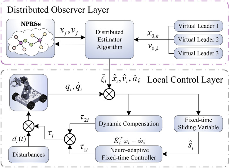
Hierarchical control framework for NPRSs.

Remark 5

The control algorithm given in (6) demonstrates considerable physical significance. To elaborate further, ${\tau }_{i,1}$ represents the robust control term for addressing the challenges posed by actuator input deadzone, parametric uncertainties, and external perturbations. ${\tau }_{i,2}$ corresponds to an equivalent control designed for NPRSs to process known information. Additionally, the update laws ${\dot{\widehat{K}}}_i={\alpha }_1{\phi }_i{\widehat{s}}_i^T$ and ${\dot{\widehat{\varpi }}}_i={\alpha }_2|{\widehat{s}}_i|$ in the neural adaptive control serve as effective approximations for dealing with the complexities introduced by the actuator input deadzone, parametric uncertainties, and external perturbations.

Remark 6

The proposed HFNA control algorithm consists of a local control layer (i.e., (6)) and a distributed observer layer (i.e., (7)). Its hierarchical architecture decomposes the control task into multiple levels, allowing each layer to handle specific aspects of the control problem. This structured decomposition enables smoother transitions between control actions, minimizing abrupt control signal changes, which helps reduce the high-frequency switching that typically leads to chattering in conventional sliding mode control. Furthermore, the adaptive neural network components continuously adjust control parameters in response to real-time system dynamics. This adaptability enables more precise and gradual modifications, mitigating the need for aggressive switching and further reducing chattering. Together, the hierarchical design and adaptive neural network enhance the robustness of the control strategy against parametric uncertainty and external perturbations, ensuring stable and reliable performance.

Analysis for the distributed observer

In this subsection, we validate the performance of the proposed distributed observer algorithm in addressing the fixed-time CFT problem.

Theorem 1

Under the assumptions of Assumption 1-3, and with the proposed distributed observer algorithm (7), if the conditions are satisfied as

$$\begin{array}{cc}& {\sigma }_{min}>0,{\eta }_{min}>0,\hfill \end{array}$$ 8

$$\begin{array}{cc}& m_1>n_1,m_2<n_2,\hfill \end{array}$$ 9

where ${\sigma }_{min}=min\{{\sigma }_1,{\sigma }_2,{\sigma }_3\}$, and ${\eta }_{min}=min\{{\eta }_1,{\eta }_2,{\eta }_3\}$. Then, the states of the virtual leaders are effectively observed within a fixed time $t\le {\mathcal{T}}_e$, i.e.,${lim}_{t\to {\mathcal{T}}_e}\Vert {\tilde{\xi }}_i\Vert =0$, and $\Vert {\tilde{\xi }}_i\Vert =0$, when$t>{\mathcal{T}}_e$, $\forall i\in \mathcal{V}$.

Proof

First, the distributed observer tracking error vectors for $i,j\in \mathcal{V}$ are defined as follows:

$$\begin{array}{c}\hfill \left\{\begin{array}{c}{\tilde{x}}_i={\widehat{x}}_i-x_{0,k},\hfill \\ {\tilde{v}}_i={\widehat{v}}_i-v_{0,k},\hfill \\ {\tilde{a}}_i={\widehat{a}}_i-a_{0,k}.\hfill \end{array}\right)\end{array}$$

Let ${\tilde{\xi }}_i=\mathrm{col}({\tilde{x}}_i,{\tilde{v}}_i,{\tilde{a}}_i)\in {\mathbb{R}}^{3d}$, the compact representations of ${\tilde{x}}_i$ , ${\tilde{v}}_i$, and ${\tilde{a}}_i$ are as follows:

$$\begin{array}{c}\hfill \left\{\begin{array}{c}\tilde{x}=\mathrm{col}({\tilde{x}}_1,{\tilde{x}}_2,\dots ,{\tilde{x}}_N)\hfill \\ \tilde{v}=\mathrm{col}({\tilde{v}}_1,{\tilde{v}}_2,\dots ,{\tilde{v}}_N)\hfill \\ \tilde{a}=\mathrm{col}({\tilde{a}}_1,{\tilde{a}}_2,\dots ,{\tilde{a}}_N)\hfill \end{array}\right)\end{array}$$

Thus, we can obtain the compact form $\tilde{\xi }=\text{col}(\tilde{x},\tilde{v},\tilde{a})$. Furthermore, substituting the proposed HFNA control algorithm (6), (7) into (5) obtains the cascade closed-loop system as follows:

$$\begin{array}{c}\hfill \left\{\begin{array}{c}\begin{array}{cc}\hfill {\dot{\widehat{s}}}_i& ={\dot{\widehat{e}}}_i+\frac{n_4}{m_4}{({ħ}_i^{-1}·{\dot{\widehat{e}}}_i)}^{\frac{n_4-m_4}{m_4}}({\mathrm{\Gamma }}_i·{\dot{\widehat{e}}}_i^2·{ħ}_i^{-2}+{ħ}_i^{-1}·{\ddot{\widehat{e}}}_i),\hfill \\ \hfill \dot{\tilde{\xi }}& ={[(\mathcal{L}+\mathcal{B})\otimes I_{3d}]}^{-1}\{-P\mathrm{sig}{([(\mathcal{L}+\mathcal{B})\otimes I_{3d}]\tilde{\xi })}^{\frac{m_1}{n_1}}\hfill \\ \hfill & -Q\mathrm{sig}{([(\mathcal{L}+\mathcal{B})\otimes I_{3d}]\tilde{\xi })}^{\frac{m_2}{n_2}}+(\mathcal{B}\otimes I_{3d}){\dot{\gamma }}_0\}-{\dot{\gamma }}_0,\hfill \end{array}\hfill \end{array}\right)\end{array}$$ 10

where ${\gamma }_0=\mathrm{col}\left(x_0,v_0,a_0\right)$,

$$\begin{array}{cc}\hfill x_0=& \mathrm{col}(\underset{n_1}{\underbrace{x_{0,1},\dots ,x_{0,1}}},\underset{n_2}{\underbrace{x_{0,2},\dots ,x_{0,2}}},\dots ,\underset{n_{\mathcal{K}}}{\underbrace{x_{0,\mathcal{K}},\dots ,x_{0,\mathcal{K}}}}),\hfill \\ \hfill v_0=& \mathrm{col}(\underset{n_1}{\underbrace{v_{0,1},\dots ,v_{0,1}}},\underset{n_2}{\underbrace{v_{0,2},\dots ,v_{0,2}}},\dots ,\underset{n_{\mathcal{K}}}{\underbrace{v_{0,\mathcal{K}},\dots ,v_{0,\mathcal{K}}}}),\hfill \\ \hfill a_0=& \mathrm{col}(\underset{n_1}{\underbrace{a_{0,1},\dots ,a_{0,1}}},\underset{n_2}{\underbrace{a_{0,2},\dots ,a_{0,2}}},\dots ,\underset{n_{\mathcal{K}}}{\underbrace{a_{0,\mathcal{K}},\dots ,a_{0,\mathcal{K}}}}).\hfill \end{array}$$

In the closed-loop system (10), given that $\dot{\tilde{\xi }}$ is defined, taking linear transformations $\tilde{\mathrm{\Phi }}=[(\mathcal{L}+\mathcal{B})\otimes I_{3d}]\tilde{\xi }$ yields

$$\begin{array}{cc}\hfill \dot{\tilde{\mathrm{\Phi }}}=& [(\mathcal{L}+\mathcal{B})\otimes I_{3d}]\dot{\tilde{\xi }}\hfill \\ \hfill =& -P\mathrm{sig}{([(\mathcal{L}+\mathcal{B})\otimes I_{3d}]\tilde{\xi })}^{\frac{m_1}{n_1}}\hfill \\ \hfill & -Q\mathrm{sig}{([(\mathcal{L}+\mathcal{B})\otimes I_{3d}]\tilde{\xi })}^{\frac{m_2}{n_2}}\hfill \\ \hfill & +(\mathcal{B}\otimes I_{3d}){\dot{\gamma }}_0-[(\mathcal{L}+\mathcal{B})\otimes I_{3d}]{\dot{\gamma }}_0.\hfill \end{array}$$ 11

It’s worth noting that $(\mathcal{B}\otimes I_{3d}){\dot{\gamma }}_0=[(\mathcal{L}+\mathcal{B})\otimes I_{3d}]{\dot{\gamma }}_0$. Then, it can be derived that

$$\begin{array}{c}\hfill \dot{\tilde{\mathrm{\Phi }}}=-P\mathrm{sig}{(\tilde{\mathrm{\Phi }})}^{\frac{m_1}{n_1}}-Q\mathrm{sig}{(\tilde{\mathrm{\Phi }})}^{\frac{m_2}{n_2}}.\end{array}$$ 12

Consider the positive-definite Lyapunov function candidate defined as

$$\begin{array}{c}\hfill V(\tilde{\mathrm{\Phi }})=\mathrm{sig}{\mathrm{n}}^T(\tilde{\mathrm{\Phi }}).\end{array}$$ 13

Further, taking the derivative of the function $V(\tilde{\mathrm{\Phi }})$, it can be derived that

$$\begin{array}{cc}\hfill \dot{V}(\tilde{\mathrm{\Phi }})\le & -{\Vert P\Vert }_1\Vert \tilde{\mathrm{\Phi }}{\Vert }_1^{\frac{m_1}{n_1}}-{∥Q∥}_1{\Vert \tilde{\mathrm{\Phi }}\Vert }_1^{\frac{m_2}{n_2}}\hfill \\ \hfill =& -{∥P∥}_1{V}^{\frac{m_1}{n_1}}(\tilde{\mathrm{\Phi }})-{∥Q∥}_1{V}^{\frac{m_2}{n_2}}(\tilde{\mathrm{\Phi }}).\hfill \end{array}$$ 14

Thus, ${\tilde{\xi }}_i=0$ when fixed-time $t\ge {\mathcal{T}}_e$ and ${\mathcal{T}}_e$ is bounded by

$$\begin{array}{c}\hfill {\mathcal{T}}_e\le {\mathcal{T}}_{emax}=\frac{1}{{\sigma }_{min}}\frac{n_1}{m_1-n_1}+\frac{1}{{\eta }_{min}}\frac{n_2}{n_2-m_2}.\end{array}$$ 15

In addition, if ${\theta }_1\stackrel{\mathrm{\Delta }}{=}[n_2(m_1-n_1)]/[n_1(n_2-m_2)]\le 1$, a less conservative approximation can be derived as follows:

$$\begin{array}{c}\hfill {\mathcal{T}}_e\le {\mathcal{T}}_{emax}=\frac{n_2}{n_2-m_2}\left(\frac{1}{\sqrt{{\sigma }_{min}{\eta }_{min}}}{tan}^{-1}\sqrt{\frac{{\sigma }_{min}}{{\eta }_{min}}}+\frac{1}{{\sigma }_{min}{\theta }_1}\right).\end{array}$$

$\square$

Remark 7

The result from Theorem 1, ${lim}_{t\to {\mathcal{T}}_e}\Vert {\tilde{\xi }}_i\Vert =0$, and $\Vert {\tilde{\xi }}_i\Vert =0$, when $t>{\mathcal{T}}_e$, and can be easily obtained ${lim}_{t\to {\mathcal{T}}_e}∥{\tilde{x}}_i∥=0$, ${lim}_{t\to {\mathcal{T}}_e}∥{\tilde{v}}_i∥=0$, ${lim}_{t\to {\mathcal{T}}_e}∥{\tilde{a}}_i∥=0$ and $∥{\tilde{x}}_i∥=0$, $∥{\tilde{v}}_i∥=0$, $∥{\tilde{a}}_i∥=0$.

Analysis of fixed-time CFT

In this subsection, we demonstrate the effectiveness of the presented algorithm in solving the fixed-time CFT problem, building upon the result established in Theorem 1.

Theorem 2

By applying the proposed HFNA control algorithm (6)–(7) to the system (5), and under the condition that

$$\begin{array}{c}\hfill {\beta }_i\ge ∥{\tilde{K}}_i^T{\phi }_i+{\tilde{\varpi }}_i∥,\forall i\in \mathcal{V},\end{array}$$ 16

where ${\tilde{K}}_i=K_i-{\widehat{K}}_i$ and ${\tilde{\varpi }}_i={\varpi }_i-{\widehat{\varpi }}_i$, the fixed-time CFT problem (Definition3) in NPRSs is successfully solved.

Proof

The theorem demonstrates that $q_i$ and $\dot{q_i}$ can track their corresponding observer terms ${\widehat{x}}_i$ and ${\widehat{v}}_i$ within a fixed time. First, the distributed tracking errors are defined as ${\widehat{e}}_i=q_i-r_i-{\widehat{x}}_i$ and ${\dot{\widehat{e}}}_i=\dot{q_i}-{\widehat{v}}_i$. The analysis then focuses on the convergence of the fixed-time sliding vector ${\widehat{s}}_i$. To facilitate this analysis, a Lyapunov function candidate is introduced, followed by a detailed convergence analysis.

$$\begin{array}{c}\hfill V_i({\widehat{s}}_i)=\frac{1}{2}{\widehat{s}}_i^T{\widehat{s}}_i,\forall i\in \mathcal{V}.\end{array}$$ 17

Consider that ${\dot{\widehat{s}}}_i$ is defined in the closed-loop system (10), the derivative of $V_i$ can be expressed as follows:

$$\begin{array}{cc}\hfill {\dot{V}}_i({\widehat{s}}_i)=& {\widehat{s}}_i^T{\dot{\widehat{s}}}_i\hfill \\ \hfill =& {\widehat{s}}_i^T[{\dot{\widehat{e}}}_i+\frac{n_4}{m_4}{({ħ}_i^{-1}·{\dot{\widehat{e}}}_i)}^{(n_4/m_4)-1}({\mathrm{\Gamma }}_i·{\dot{\widehat{e}}}_i^2·{ħ}_i^{-2}\hfill \\ \hfill & +{ħ}_i^{-1}·{\ddot{\widehat{e}}}_i)],\hfill \\ \hfill & ={\widehat{s}}_i^T\{{\dot{\widehat{e}}}_i+\frac{n_4}{m_4}{({ħ}_i^{-1}·{\dot{\widehat{e}}}_i)}^{(n_4/m_4)-1}\{{\mathrm{\Gamma }}_i·{\dot{\widehat{e}}}_i^2·{ħ}_i^{-2}\hfill \\ \hfill & +{ħ}_i^{-1}·[{H_{i0}}^{-1}({\tau }_i+K_i^T{\phi }_i+{\epsilon }_i\hfill \\ \hfill & -C_{i0}{\dot{q}}_i-G_{i0})-{\widehat{a}}_i]\}\}\hfill \end{array}$$ 18

where ${\mathrm{\Gamma }}_i=-{\sigma }_0[(m_3/n_3)-(m_4/n_4)]{\widehat{e}}_i^{(m_3/n_3)-(m_4/n_4)-1}$. Then, (18) can be rewritten as

$$\begin{array}{cc}\hfill {\dot{V}}_i({\widehat{s}}_i)=& \frac{n_4}{m_4}{({ħ}_i^{-1}·{\dot{\widehat{e}}}_i)}^{(n_4/m_4)-1}{\widehat{s}}_i^T[{H_{i0}}^{-1}{ħ}_i^{-1}·(K_i^T{\phi }_i\hfill \\ \hfill & +{\epsilon }_i-{\widehat{K}}_i^T{\phi }_i-{\widehat{\varpi }}_i-{\beta }_i\mathrm{sig}({\widehat{s}}_i))]-{\widehat{s}}_i^T{\delta }_i\hfill \\ \hfill \le & {\widehat{s}}_i^T[{H_{i0}}^{-1}{ħ}_i^{-1}·(K_i^T{\phi }_i+{\varpi }_i-{\widehat{K}}_i^T{\phi }_i-{\widehat{\varpi }}_i\hfill \\ \hfill & -{\beta }_i\mathrm{sig}({\widehat{s}}_i))]-{\widehat{s}}_i^T{\delta }_i\hfill \\ \hfill \le & {\widehat{s}}_i^T[{H_{i0}}^{-1}{ħ}_i^{-1}·({\tilde{K}}_i^T{\phi }_i+{\tilde{\varpi }}_i-{\beta }_i\mathrm{sig}({\widehat{s}}_i))]\hfill \\ \hfill & -{\widehat{s}}_i^T{\delta }_i,\hfill \end{array}$$ 19

where $∥{\epsilon }_i∥\le {\varpi }_i$ is defined in (4). In accordance with (16), we obtain that

$$\begin{array}{cc}\hfill {\dot{V}}_i({\widehat{s}}_i)& \le -{\widehat{s}}_i^T{\delta }_i\hfill \\ \hfill & \le -{\widehat{s}}_i^T({\sigma }_4{\widehat{s}}_i^{m_3/n_3}+{\eta }_4{\widehat{s}}_i^{m_4/n_4})\hfill \\ \hfill & \le 0,\hfill \end{array}$$ 20

where ${\delta }_i={\sigma }_4{\widehat{s}}_i^{m_3/n_3}+{\eta }_4{\widehat{s}}_i^{m_4/n_4}$ is defined in (6). The inequality above indicates that ${\dot{V}}_i({\widehat{s}}_i)$ is negative definite, ensuring the convergence of ${\widehat{s}}_i$ for all $i\in \mathcal{V}$. Alternatively, the selected Lyapunov function candidate is as follows for the neural adaptive laws:

$$\begin{array}{c}\hfill V_i({\tilde{K}}_i,{\tilde{\varpi }}_i)=\frac{1}{2}\mathrm{tr}({\tilde{K}}_i^T{\alpha }_1^{-1}{\tilde{K}}_i)+\frac{1}{2}{\alpha }_2^{-1}{\tilde{\varpi }}_i^2.\end{array}$$ 21

Given the positive constants ${\alpha }_1$ and ${\alpha }_2$, the function $V_i({\tilde{K}}_i,{\tilde{\varpi }}_i)$ is positive definite. Furthermore, we can deduce from (6), (16), and the previous analysis that ${\tilde{K}}_i,{\tilde{\varpi }}_i\in L_2\cap L\infty$ and ${\dot{\tilde{K}}}_i,{\dot{\tilde{\varpi }}}_i\in L\infty$. The derivative of $V_i({\tilde{K}}_i,{\tilde{\varpi }}_i)$ is then expressed as follows:

$$\begin{array}{c}\hfill {\dot{V}}_i({\tilde{K}}_i,{\tilde{\varpi }}_i)=-\mathrm{tr}({\tilde{K}}_i^T({\phi }_i{\widehat{s}}_i^T))-{\tilde{\varpi }}_i∥{\widehat{s}}_i∥.\end{array}$$ 22

Thus, it follows that

$$\begin{array}{c}\hfill {\ddot{V}}_i({\tilde{K}}_i,{\tilde{\varpi }}_i)=\mathrm{tr}({\alpha }_1{\widehat{s}}_i{\phi }_i^T({\phi }_i{\widehat{s}}_i^T))+\mathrm{tr}({\tilde{K}}_i^T({\dot{\phi }}_i{\dot{\widehat{s}}}_i^T)+{\alpha }_2\Vert {\dot{\widehat{s}}}_i\Vert .\end{array}$$ 23

On the basis of the analysis of (19) and (20), which shows that ${\widehat{s}}_i\in L_2\cap L_{\infty }$, and considering the closed-loop dynamics (10), we can conclude that ${\dot{\widehat{s}}}_i\in L_{\infty }$. Additionally, the boundedness of ${\dot{\phi }}_i$ defined in (4) implies that ${\ddot{V}}_i({\tilde{K}}_i,{\tilde{\varpi }}_i)\in L_{\infty }$. By applying Barbalat’s lemma¹⁰ and combining it with the previous analysis, we further deduce that ${\tilde{K}}_i\to 0$ and ${\tilde{\varpi }}_i\to 0$ as $t\to \infty$. This finding demonstrates the effectiveness of the neural adaptive law, allowing the use of smaller ${\beta }_i$ and reducing the chattering phenomenon.

With regard to (16), obtaining knowledge of ${\tilde{\varpi }}_i$ may be challenging in practical applications. In such scenarios, a practical solution is to choose a suitably large ${\beta }_i$ to ensure the stability condition. This solution results in the following reformulation of (19):

$$\begin{array}{cc}\hfill {\dot{V}}_i({\widehat{s}}_i)\le & -{\widehat{s}}_i^T({\sigma }_4{\widehat{s}}_i^{m_3/n_3}+{\eta }_4{\widehat{s}}_i^{m_4/n_4})\hfill \\ \hfill \le & -{\sigma }_4{\widehat{s}}_i^{(m_3+n_3)/n_3}-{\eta }_4{\widehat{s}}_i^{(m_4+n_4)/n_4}\hfill \\ \hfill \le & -{\sigma }_4{2}^{(m_3+n_3)/2n_3}{V}_i{({\widehat{s}}_i)}^{(m_3+n_3)/2n_3}\hfill \\ \hfill & -{\eta }_4{2}^{(m_4+n_4)/2n_4}{V}_i{({\widehat{s}}_i)}^{(m_4+n_4)/2n_4}.\hfill \end{array}$$ 24

By utilizing Lemma 1 and the expression in (24), the distributed tracking errors ${\widehat{e}}_i=q_i-r_i-{\widehat{x}}_i$ and ${\dot{\widehat{e}}}_i={\dot{q}}_i-{\widehat{v}}_i$ evidently reach the manifold ${\widehat{s}}_i$ within the fixed time $t\le {\mathcal{T}}_{l,1}$. Then, ${\mathcal{T}}_{l,1}$ is defined as follows:

$$\begin{array}{c}\hfill {\mathcal{T}}_{l,1}\le {\mathcal{T}}_{lmax,1}=\frac{2^{(n_3-m_3)/2n_3}}{{\sigma }_4}\frac{n_3}{m_3-n_3}+\frac{2^{(n_4-m_4)/2n_4}}{{\eta }_4}\frac{n_4}{n_4-m_4}.\end{array}$$ 25

Drawing upon the preceding analysis and fixed-time sliding mode control theory²², a conclusion can be readily drawn that ${\widehat{e}}_i$ and ${\dot{\widehat{e}}}_i$ achieve convergence to the origin within the fixed time ${\mathcal{T}}_l\le {\mathcal{T}}_{lmax,1}+{\mathcal{T}}_{lmax,2}$. In particular, it follows from (25) that

$$\begin{array}{cc}\hfill {\mathcal{T}}_l\le & {\mathcal{T}}_{lmax,1}+{\mathcal{T}}_{lmax,2}\hfill \\ \hfill =& {\mathcal{T}}_{lmax,1}+\frac{1}{{\sigma }_0}\frac{n_3}{m_3-n_3}+\frac{1}{{\eta }_0}\frac{n_4}{n_4-m_4}\hfill \\ \hfill =& \frac{n_3}{m_3-n_3}\left(\frac{2^{(n_3-m_3)/2n_3}}{{\sigma }_4}+\frac{1}{{\sigma }_0}\right)\hfill \\ \hfill & +\frac{n_4}{n_4-m_4}\left(\frac{2^{(n_4-m_4)/2n_4}}{{\eta }_4}+\frac{1}{{\eta }_0}\right).\hfill \end{array}$$ 26

In addition, if ${\theta }_2\stackrel{\mathrm{\Delta }}{=}[n_4(m_3-n_3)]/[n_3(n_4-m_4)]\le 1$, a less conservative bound can be obtained as

$$\begin{array}{cc}\hfill {\mathcal{T}}_l\le & \frac{n_4}{n_4-m_4}\left(\frac{1}{\sqrt{{\sigma }_0{\eta }_0}}{tan}^{-1}\sqrt{\frac{{\sigma }_0}{{\eta }_0}}+\frac{1}{{\sigma }_0{\theta }_2}\right)\hfill \\ \hfill & \left(+\frac{1}{\sqrt{{\sigma }_4{\eta }_4}}{tan}^{-1}\sqrt{\frac{{\sigma }_4}{{\eta }_4}}+\frac{2^{-(n_3+m_3)/2n_3}}{{\sigma }_4{\theta }_2}\right).\hfill \end{array}$$ 27

The second step validates the successful resolution of the fixed-time CFT problem. Before proceeding, let $e_i=q_i-r_i-x_{0,k}$ and ${\dot{e}}_i={\dot{q}}_i-v_{0,k}$, where $e_i$ and ${\dot{e}}_i$ represent the position and velocity tracking errors of the robots, respectively. Applying the Triangle Inequality, it can be obtained that

$$\begin{array}{cc}\hfill \underset{t\to {\mathcal{T}}_f}{lim}∥e_i∥=& \underset{t\to {\mathcal{T}}_f}{lim}∥(q_i-r_i-{\widehat{x}}_i)+({\widehat{x}}_i-x_{0,k})∥\hfill \\ \hfill \le & \underset{t\to {\mathcal{T}}_f}{lim}∥{\widehat{e}}_i∥+\underset{t\to {\mathcal{T}}_f}{lim}∥{\tilde{x}}_i∥\hfill \\ \hfill \le & 0,\hfill \\ \hfill \underset{t\to {\mathcal{T}}_f}{lim}∥{\dot{e}}_i∥=& \underset{t\to {\mathcal{T}}_f}{lim}∥({\dot{q}}_i-{\widehat{v}}_i)+({\widehat{v}}_i-x_{0,k})∥\hfill \\ \hfill \le & \underset{t\to {\mathcal{T}}_f}{lim}∥{\dot{\widehat{e}}}_i∥+\underset{t\to {\mathcal{T}}_f}{lim}∥{\tilde{v}}_i∥\hfill \\ \hfill \le & 0,\hfill \end{array}$$

where ${\mathcal{T}}_f\le {\mathcal{T}}_e+{\mathcal{T}}_l$. Therefore, the problem defined in Definition 3 is effectively resolved, concluding the proof. $\square$

Remark 8

We choose ${\mathcal{T}}_f\le {\mathcal{T}}_e+{\mathcal{T}}_l$ to represent the total time required for system convergence, which includes the time ${\mathcal{T}}_e$ associated with the distributed observer layer and the time ${\mathcal{T}}_l$ related to the local control layer. This approach ensures that the cumulative nature of the convergence times across different stages is fully considered, encompassing all phases of the convergence process. By contrast, using ${\mathcal{T}}_f\le max({\mathcal{T}}_e,{\mathcal{T}}_l)$ would imply that the convergence time is determined solely by the longer duration of either the distributed observer layer or the local control layer. This choice assumes that one stage completes immediately after the other, disregarding potential overlaps or the possibility of collaborative convergence between the stages.

Simulations

This section depicts the efficacy of the HFNA control algorithm outlined in Algorithm 1 through simulation.

Algorithm 1.

HFNA control

The NPRS comprises ten identical follower robots (2-DOF) and three virtual leaders (simplified leader representations). Moreover, the interactions of the NPRS are illustrated in Fig. 4. The Laplacian matrix $\mathcal{L}$ can be computed as

$$\begin{array}{c}\hfill \mathcal{L}=\left[\begin{array}{cccccccccc}2& 0& -2& 0& 0& 0& 0& 0& 0& 0\\ -1& 1& 0& 0& 0& 0& 0& 0& 0& 0\\ -2& 0& 2& -4& 0& 4& 0& 0& 0& 0\\ 0& 0& 0& 1& -1& 0& 0& 0& 0& 0\\ 0& 0& 0& 0& 3& 0& -3& 0& 0& 0\\ 0& 0& 0& -2& 0& 3& -1& 0& 0& 0\\ 0& 0& 0& 0& -3& 0& 3& -2& 0& 2\\ 0& 0& 0& 0& 0& 0& 0& 1& 0& -1\\ 0& 0& 0& 0& 0& 0& 0& -2& 2& 0\\ 0& 0& 0& 0& 0& 0& 0& 0& -1& 1\end{array}\right].\end{array}$$

Additionally, the physical parameters of the NPRS are selected in Table 1. The observations of the physical parameters of the NPRS are selected in Table 2. The dynamics descriptions is given by

$$\begin{array}{cc}& \left[\begin{array}{cc}{H}_{i11}& H_{i12}\\ H_{i21}& H_{i22}\end{array}\right]\left[\begin{array}{c}{\ddot{q}}_{i1}\\ {\ddot{q}}_{i2}\end{array}\right]+\left[\begin{array}{cc}{C}_{i11}& C_{i12}\\ C_{i21}& C_{i22}\end{array}\right]\left[\begin{array}{c}{\dot{q}}_{i1}\\ {\dot{q}}_{i2}\end{array}\right]\hfill \\ \hfill & +\left[\begin{array}{c}{G}_{i1}\\ G_{i2}\end{array}\right]+\left[\begin{array}{c}{d}_{i1}\\ d_{i2}\end{array}\right]=\left[\begin{array}{c}\psi ({\tau }_{i1})\\ \psi ({\tau }_{i2})\end{array}\right].\hfill \end{array}$$

In more detail, $H_{i11}=\overline{\phantom{n}}{\lambda }_{i1}+2\overline{\phantom{n}}{\lambda }_{i2}cos({\dot{q}}_{i2})$, $H_{i12}=H_{i21}=\overline{\phantom{n}}{\lambda }_{i3}+2\overline{\phantom{n}}{\lambda }_{i2}cos({\dot{q}}_{i2})$, $H_{i22}=\overline{\phantom{n}}{\lambda }_{i2}$, $C_{i12}=-\overline{\phantom{n}}{\lambda }_{i2}sin({\dot{q}}_{i2})({\dot{q}}_{i1}+{\dot{q}}_{i2})$ $C_{i21}=-\overline{\phantom{n}}{\lambda }_{i2}sin({\dot{q}}_{i2}){\dot{q}}_{i1}$, $C_{i22}=0$, $G_{i2}=g\overline{\phantom{n}}{\lambda }_{i5}cos({\dot{q}}_{i1}+{\dot{q}}_{i2})$. We select the standard gravitational torque as $g=9.8\phantom{i}\mathrm{m}/{\mathrm{s}}^2$. Furthermore, the detailed description of the corresponding parameters is provided below. $\overline{\phantom{n}}{\lambda }_{i1}$ to $\overline{\phantom{n}}{\lambda }_{i5}$ are given as $\overline{\phantom{n}}{\lambda }_{i1}=m_{i1}{\chi }_{i1}^2+m_{i2}(l_{i1}^2+{\chi }_{i2}^2)+I_{i1}+I_{i2}$, $\overline{\phantom{n}}{\lambda }_{i2}=m_{i2}{l}_{i1}{\chi }_{i2}$, $\overline{\phantom{n}}{\lambda }_{i3}=m_{i2}{\chi }_{i2}^2+I_{i2}$, $\overline{\phantom{n}}{\lambda }_{i4}=m_{i1}{\chi }_{i1}+m_{i2}{l}_{i1}$, $\overline{\phantom{n}}{\lambda }_{i5}=m_{i2}{\chi }_{i2}$, and $I_{i1}=\frac{1}{3}{m}_{i1}{l}_{i1}^2$, $I_{i2}=\frac{1}{3}{m}_{i2}{l}_{i2}^2$.

Fig. 4.

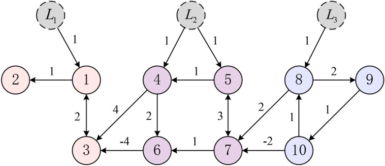
Directed graph $\mathcal{G}$ representing the NPRS network.

Table 1.

Physical parameters of the robot.

Mass ($\mathrm{kg}$)	Length ($\mathrm{m}$)	COM ($\mathrm{m}$)
$m_i={(m_{i1},m_{i2})}^T$	$l_{i1}={(l_{i1},l_{i2})}^T$	${\chi }_{i2}={({\chi }_{i1},{\chi }_{i2})}^T$
$m_{i1}=1.26+0.03i$	$l_{i1}=2.68+0.04i$	${\chi }_{i1}=1.34+0.02i$
$m_{i2}=1.04+0.02i$	$l_{i2}=2.44+0.02i$	${\chi }_{i2}=1.22+0.01i$

Table 2.

The observations of the physical parameters.

Mass ($\mathrm{kg}$)	Length ($\mathrm{m}$)	COM ($\mathrm{m}$)
${\widehat{m}}_i={({\widehat{m}}_{i1},{\widehat{m}}_{i2})}^T$	${\widehat{l}}_{i1}={({\widehat{l}}_{i1},{\widehat{l}}_{i2})}^T$	${\widehat{\chi }}_{i2}={({\widehat{\chi }}_{i1},{\widehat{\chi }}_{i2})}^T$
${\widehat{m}}_{i1}=1.16+0.03i$	${\widehat{l}}_{i1}=2.58+0.04i$	${\widehat{\chi }}_{i1}=1.24+0.02i$
${\widehat{m}}_{i2}=1.14+0.02i$	${\widehat{l}}_{i2}=2.54+0.02i$	${\widehat{\chi }}_{i2}=1.12+0.01i$

Under Assumption 3, the trajectory of the virtual leaders, labeled as $L_1$, $L_2$, and $L_3$, are selected as

$$\begin{array}{c}\hfill \left\{\begin{array}{c}{x}_{0,1}=\mathrm{col}(0.9+0.4sin(0.4t),1.0+0.4cos(0.4t)),\hfill \\ v_{0,1}=\mathrm{col}({0.4}^{2}cos(0.4t),-{0.4}^{2}sin(0.4t)),\hfill \\ a_{0,1}=\mathrm{col}(-{0.4}^{3}sin(0.4t),-{0.4}^{3}cos(0.4t)),\hfill \end{array}\right)\\ \hfill \left\{\begin{array}{c}{x}_{0,2}=\mathrm{col}(2.6+0.5cos(0.5t),1.4+0.5sin(0.5t)),\hfill \\ v_{0,2}=\mathrm{col}(-{0.5}^{2}sin(0.5t),{0.5}^{2}cos(0.5t)),\hfill \\ a_{0,2}=\mathrm{col}(-{0.5}^{3}cos(0.5t),-{0.5}^{3}sin(0.5t)),\hfill \end{array}\right)\\ \hfill \left\{\begin{array}{c}{x}_{0,3}=\mathrm{col}(1.6+0.3sin(0.3t),2.6+0.3cos(0.3t)),\hfill \\ v_{0,3}=\mathrm{col}({0.3}^{2}cos(0.3t),-{0.3}^{2}sin(0.3t)),\hfill \\ a_{0,3}=\mathrm{col}(-{0.3}^{3}sin(0.3t),-{0.3}^{3}cos(0.3t)).\hfill \end{array}\right)\end{array}$$

Furthermore, we present the parameters used in the HFNA control algorithm (6)–(7). To ensure the establishment of (8) and (9), the following parameter values are used: ${\sigma }_{min}=8$ (${\sigma }_1=8$, ${\sigma }_2=9$, ${\sigma }_3=10$), ${\eta }_{min}=8$ (${\eta }_1=8$, ${\eta }_2=9$, ${\eta }_3=10$), $m_1=2$, $n_1=1$, $m_2=1$, and $n_2=2$. Besides, the parameters of the neural adaptive laws are specified as ${\alpha }_1=0.1$ and ${\alpha }_2=1.01$. The neural networks ${\widehat{K}}_i^T{\phi }_i$ comprise 10 neurons, where the centers ${\rho }_i$ are evenly distributed in the range $[-2\pi ,2\pi ]$, with widths ${\iota }_i=20$. We choose ${\sigma }_0=1,{\eta }_0=1,{\sigma }_4=1,{\eta }_4=1$, $n_3=5$, $m_4=7$ and $n_4=9$, ${\beta }_i=50$ to make (16) holds. Furthermore, the external perturbations is chosen as $d_i(t)=-0.1\mathrm{col}(cost,sint)$. Besides, the formation offsets are set to $r_1=\mathrm{col}(0,2/9)\text{m}$, $r_3=\mathrm{col}(\sqrt{3}/9,-1/9)\text{m}$, $r_4=\mathrm{col}(-0.16,0.15)\text{m}$, $r_5=\mathrm{col}(0.15,0.15)\text{m}$, $r_6=\mathrm{col}(0.15,-0.15)\text{m}$, $r_7=\mathrm{col}(-0.15,-0.15)\text{m}$, $r_8=\mathrm{col}(0,1/4)\text{m}$, $r_9=\mathrm{col}(-\sqrt{3}/8,-1/8)\text{m}$, $r_{10}=\mathrm{col}(\sqrt{3}/8,-1/8)\text{m}$. Here, the input deadzone function of the robotic manipulator is denoted as

$$\begin{array}{c}\hfill \psi ({\tau }_i)=\left\{\begin{array}{c}{\tau }_i-\text{col}(10,10),∥{\tau }_i∥\ge 10,\hfill \\ 0,-10<∥{\tau }_i∥<10,\hfill \\ {\tau }_i+\text{col}(10,10),∥{\tau }_i∥\le -10.\hfill \end{array}\right)\end{array}$$

The initial states $q_i\left(0\right)$ and ${\dot{q}}_i\left(0\right)$ are randomly assigned within the ranges of $[-5,5]$ and $[-0.2,0.2]$, respectively.

Remark 9

The comparative analysis provided in Table 3 offers a thorough evaluation of our proposed control algorithm in relation to several established methods^{20,33,34,37,38}. This analysis emphasizes the advantages of our approach, particularly in key performance areas such as convergence time, hierarchical control, deadzone compensation, uncertainty treatment, and formation task. By highlighting these aspects, we demonstrate the practical benefits of our method, ensuring a more comprehensive understanding of its effectiveness in addressing complex control challenges.

Table 3.

Comparison of related literature.

References	CT	HC	DC	UT	FT
Meng et al.20	Finite	No	No	Fuzzy	No
Shi and Hu33	Finite	Yes	No	No	No
Cheng et al.34	Fixed	No	No	Observer	Single
Ding et al.37	Practical fixed	Yes	No	Observer	Cluster
Yoo and Park38	Fixed	No	No	No	Single
Our	Fixed	Yes	Yes	RBF	Cluster

CT convergence time, HC hierarchical control, DC deadzone compensation, UT uncertainty treatment, FT formation task.

$\mathbf{Simulation}$ $\mathbf{results}$ are presented in Figs. 5, 6, 7, 8, 9, 10 and 11, depicting the fixed-time CFT trajectories of the NPRS on the XY plane for 10 robots (Fig. 5). The efficacy of the proposed HFNA control algorithm (6)–(7) in achieving excellent fixed-time CFT performance of the NPRS is evident from the outcomes. In detail, from (c)–(d) in Figs. 6 and 7, the position observers ${\widehat{x}}_i$ converge to $x_{0,k}$ for all $i\in {\mathcal{V}}_k,k\in 1,2,3$ within the fixed time ${\mathcal{T}}_e$. Additionally, (a)–(b) in Figs. 6 and 7 reveal the attainment of fixed-time convergence of $q_i$, $i\in \mathcal{V}$, through the designed HFNA control algorithm. Using the parameters we set, the fixed settling time of the distributed observer layer $t\le {\mathcal{T}}_e=0.38\text{s}$ (based on (15)), and the fixed settling time of the local layer $t\le {\mathcal{T}}_l=9.36\text{s}$ (based on (26)). Therefore, the total fixed-time convergence is ${\mathcal{T}}_f\le {\mathcal{T}}_e+{\mathcal{T}}_l=9.74\text{s}$. Meanwhile, from Fig. 7, $e_i$ for $i\in \mathcal{V}$ are bounded within the range of $[-0.1,0.1]$ in a fixed time $t\approx 4.50\text{s}<{\mathcal{T}}_f$. Similarly, Fig. 8 demonstrates the tracking performance of the velocities. Additionally, Fig. 9 provides evidence of the stability of the neural adaptive parameters. Figure 10 illustrates the evolution of the RBF neural network approximation error. As shown, the neural network approximation error ${\epsilon }_i$ gradually converges to zero. This result demonstrates that the RBF network effectively approximates the lumped uncertainties, thereby ensuring the accuracy of the control algorithm and the stability of the overall system. In Fig. 11b, the control input torque ${\tau }_1$ for the 1st robot is bounded, minimizing the impact of minor input fluctuations and resulting in smoother control inputs as well as improved overall system performance. Overall, the simulation results validate the effectiveness and accuracy of the HFNA control algorithm.

Fig. 5.

Trajectories of NHRS with a constant cluster formation configuration under different initial conditions. Note: The intersections of the trajectories in this figure do not occur simultaneously. The robots do not occupy the same position at the same time, hence avoiding any potential collisions.

Fig. 6.

(a, b) Illustrate the evolution of the error term ($q_i-r_i$), representing the difference between the actual and reference trajectories. (c, d) display the evolution of the observed state ${\widehat{x}}_i$, showing how the state observation evolves over time.

Fig. 7.

(a, b) Show the overall position error $e_i$, illustrating the deviation between the actual and desired positions. (c, d) describe the evolution of the state observation error ${\tilde{x}}_i$ in the distributed observer layer. Finally, (e, f) display the evolution of the position error ${\widehat{e}}_i$ in the local control layer.

Fig. 8.

(a, b) Illustrate the velocity errors associated with cluster formation tracking, highlighting the discrepancies between the desired and actual velocities of the robots throughout the formation process.

Fig. 9.

(a, b) Illustrate the neural adaptive parameters of the 1st subnetwork. (c, d) display the neural adaptive parameters of the 2nd subnetwork. (e, f) present the neural adaptive parameters of the 3rd subnetwork.

Fig. 10.

(a, b) illustrate the convergence of the RBF neural network approximation error ${\epsilon }_i$ during the approximation of $F_i(t)$ for coordinates 1 and 2.

Fig. 11.

(a) Control input torque ${\tau }_i$ for coordinates 1 and 2 of the first robot without considering actuator input deadzone compensation. The comparison algorithm applied in the figure (a) is derived from reference²³. (b) Control input torque ${\tau }_i$ for coordinates 1 and 2 of the first robot while considering actuator input deadzone compensation.

Conclusion

The fixed-time CFT control problem in NPRSs was successfully addressed by considering actuator input deadzone, parametric uncertainties, and external perturbations. To address this challenging problem, a novel HFNA control algorithm, which comprised a distributed observer algorithm and a neural-adaptive fixed-time controller in the local control layer, was proposed. The simulation results demonstrated that the robots in a NPRS effectively achieved the fixed-time CFT control task, validating the feasibility of the HFNA control algorithm. Furthermore, the bipartite CFT control problem of NPRSs, which incorporates cooperative and antagonistic interconnections, can handle more complex control tasks. Consequently, our future work will be dedicated to exploring the CFT control for bipartite consensus and mobile manipulators.

Author contributions

X.L., K.-L.H., J.-Z.X.: Conceptualization, Methodology, Investigation and Validation. X.L., C.-D.L., Q.C.: Writing-original draft, Formal analysis. M.-F.G., K.-L.H., C.-D.L.: Supervision, Writing-Review & Editing.

Data availability

Simulation programmes are available from the corresponding author on reasonable request.

Declarations

Competing interests

The authors declare that there are no conflict of interest.

References

- 1.Olfati-Saber, R. & Murray, R. M. Consensus problems in networks of agents with switching topology and time-delays. IEEE Trans. Automatic Control49(9), 1520–1533. 10.1109/TAC.2004.834113 (2004). [Google Scholar]
- 2.Jin, X., Lü, S. & Yu, J. Adaptive NN-based consensus for a class of nonlinear multiagent systems with actuator faults and faulty networks. IEEE Trans. Neural Netw. Learn. Syst.33(8), 3474–3486. 10.1109/TNNLS.2021.3053112 (2021). [DOI] [PubMed] [Google Scholar]
- 3.Stiti, C. et al. Lyapunov-based neural network model predictive control using metaheuristic optimization approach. Sci. Rep.14(1), 18760. 10.1038/s41598-024-69365-9 (2024). [DOI] [PMC free article] [PubMed] [Google Scholar]
- 4.Deng, C., Wen, C., Wang, W., Li, X. & Yue, D. Distributed adaptive tracking control for high-order nonlinear multiagent systems over event-triggered communication. IEEE Trans. Autom. Control68(2), 1176–1183. 10.1109/TAC.2022.3148384 (2022). [Google Scholar]
- 5.Tang, M., Tang, K., Zhang, Y., Qiu, J. & Chen, X. Motion/force coordinated trajectory tracking control of nonholonomic wheeled mobile robot via LMPC-AISMC strategy. Sci. Rep.14(1), 18504. 10.1038/s41598-024-68757-1 (2024). [DOI] [PMC free article] [PubMed] [Google Scholar]
- 6.Li, W., Zhang, H., Cai, Y. & Wang, Y. Fully distributed formation control of general linear multiagent systems using a novel mixed self-and event-triggered strategy. IEEE Trans. Syst. Man Cybern. Syst.52(9), 5736–5745. 10.1109/TSMC.2021.3129469 (2021). [Google Scholar]
- 7.Cajo, R. et al. Distributed formation control for multiagent systems using a fractional-order proportional-integral structure. IEEE Trans. Control Syst. Technol.29(6), 2738–2745. 10.1109/TCST.2021.3053541 (2021). [Google Scholar]
- 8.Liu, Y., Zhang, H., Shi, Z. & Gao, Z. Neural-network-based finite-time bipartite containment control for fractional-order multi-agent systems. IEEE Trans. Neural Netw. Learn. Syst.34(10), 7418–7429. 10.1109/TNNLS.2022.3143494 (2023). [DOI] [PubMed] [Google Scholar]
- 9.Xiao, J., Yuan, G., He, J., Fang, K. & Wang, Z. Graph attention mechanism based reinforcement learning for multi-agent flocking control in communication-restricted environment. Inf. Sci.620, 142–157. 10.1016/j.ins.2022.11.059 (2023). [Google Scholar]
- 10.Li, Y., Li, Y. X. & Tong, S. Event-based finite-time control for nonlinear multi-agent systems with asymptotic tracking. IEEE Trans. Autom. Control68(6), 3790–3797. 10.1109/TAC.2022.3197562 (2023). [Google Scholar]
- 11.Dong, Y. & Chen, Z. Fixed-time synchronization of networked uncertain Euler–Lagrange systems. Automatica146, 110571. 10.1016/j.automatica.2022.110571 (2022). [Google Scholar]
- 12.Ding, T. F., Ge, M. F., Xiong, C. H., Park, J. H. & Li, M. Second-order bipartite consensus for networked robotic systems with quantized-data interactions and time-varying transmission delays. ISA Trans.108, 178–187. 10.1016/j.isatra.2020.08.026 (2021). [DOI] [PubMed] [Google Scholar]
- 13.Zhang, Y., Kong, L., Zhang, S., Yu, X. & Liu, Y. Improved sliding mode control for a robotic manipulator with input deadzone and deferred constraint. IEEE Trans. Syst. Man Cybern. Syst.53(12), 7814–7826. 10.1109/TSMC.2023.3301662 (2023). [Google Scholar]
- 14.Wu, Y., Niu, W., Kong, L., Yu, X. & He, W. Fixed-time neural network control of a robotic manipulator with input Deadzone. IEEE Trans. Syst. Man Cybern. Syst.135, 449–461. 10.1016/j.isatra.2022.09.030 (2023). [DOI] [PubMed] [Google Scholar]
- 15.Zhang, J., Zhang, H., Zhang, K. & Cai, Y. Observer-based output feedback event-triggered adaptive control for linear multiagent systems under switching topologies. IEEE Trans. Neural Netw. Learn. Syst.33(12), 7161–7171. 10.1109/TNNLS.2021.3084317 (2021). [DOI] [PubMed] [Google Scholar]
- 16.Li, Y., Li, K. & Tong, S. An observer-based fuzzy adaptive consensus control method for nonlinear multiagent systems. IEEE Trans. Fuzzy Syst.30(11), 4667–4678. 10.1109/TFUZZ.2022.3154433 (2022). [Google Scholar]
- 17.Yang, R., Liu, L. & Feng, G. Event-triggered robust control for output consensus of unknown discrete-time multiagent systems with unmodeled dynamics. IEEE Trans. Cyber.52(7), 6872–6885. 10.1109/TCYB.2020.3034697 (2020). [DOI] [PubMed] [Google Scholar]
- 18.Jin, Z., Wang, Z. & Zhang, X. Cooperative control problem of Takagi–Sugeno fuzzy multiagent systems via observer based distributed adaptive sliding mode control. J. Franklin Inst.359(8), 3405–3426. 10.1016/j.jfranklin.2022.03.024 (2022). [Google Scholar]
- 19.Liu, Y., Zhu, Q., Zhao, N. & Wang, L. Fuzzy approximation-based adaptive finite-time control for nonstrict feedback nonlinear systems with state constraints. Inf. Sci.548, 101–117. 10.1016/j.ins.2020.09.042 (2021). [Google Scholar]
- 20.Meng, B., Liu, W. & Qi, X. Disturbance and state observer-based adaptive finite-time control for quantized nonlinear systems with unknown control directions. J. Franklin Inst.359(7), 2906–2931. 10.1016/j.jfranklin.2022.02.033 (2022). [Google Scholar]
- 21.He, W. J., Zhu, S. L., Li, N. & Han, Y. Q. Adaptive finite-time control for switched nonlinear systems subject to multiple objective constraints via multi-dimensional Taylor network approach. ISA Trans.136, 323–333. 10.1016/j.isatra.2022.10.048 (2023). [DOI] [PubMed] [Google Scholar]
- 22.Zuo, Z., Tian, B., Defoort, M. & Ding, Z. Fixed-time consensus tracking for multiagent systems with high-order integrator dynamics. IEEE Trans. Autom. Control63(2), 563–570. 10.1109/TAC.2017.2729502 (2017). [Google Scholar]
- 23.Xu, J. Z., Ge, M. F., Ding, T. F., Liang, C. D. & Liu, Z. W. Neuro-adaptive fixed-time trajectory tracking control for human-in-the-loop teleoperation with mixed communication delays. IET Control Theory Appl.14(19), 3193–3203. 10.1049/iet-cta.2019.1479 (2020). [Google Scholar]
- 24.Polyakov, A., Efimov, D. & Perruquetti, W. Finite-time and fixed-time stabilization: Implicit Lyapunov function approach. Automatica51, 332–340. 10.1016/j.automatica.2014.10.082 (2015). [Google Scholar]
- 25.Koo, Y. C., Mahyuddin, M. N. & Ab Wahab, M. N. Novel control theoretic consensus-based time synchronization algorithm for WSN in industrial applications: Convergence analysis and performance characterization. IEEE Sens. J.23(4), 4159–4175. 10.1109/JSEN.2022.3231726 (2023). [Google Scholar]
- 26.Bai, W., Liu, P. X. & Wang, H. Neural-network-based adaptive fixed-time control for nonlinear multiagent non-affine systems. IEEE Trans. Neural Netw. Learn. Syst.35(1), 570–583. 10.1109/TNNLS.2022.3175929 (2024). [DOI] [PubMed] [Google Scholar]
- 27.Polyakov, A. & Krstic, M. Finite-and fixed-time nonovershooting stabilizers and safety filters by homogeneous feedback. IEEE Trans. Autom. Control68(11), 6434–6449. 10.1109/TAC.2023.3237482 (2023). [Google Scholar]
- 28.Liu, W. & Zhao, T. An active disturbance rejection control for hysteresis compensation based on neural networks adaptive control. ISA Trans.109, 81–88. 10.1016/j.isatra.2020.10.019 (2021). [DOI] [PubMed] [Google Scholar]
- 29.Guo, Q. & Chen, Z. Neural adaptive control of single-rod electrohydraulic system with lumped uncertainty. Mech. Syst. Signal Process.146, 106869. 10.1016/j.ymssp.2020.106869 (2021). [Google Scholar]
- 30.Cao, L., Cheng, Z., Liu, Y. & Li, H. Event-based adaptive NN fixed-time cooperative formation for multiagent systems. IEEE Trans. Neural Netw. Learn. Syst.35(5), 6467–6477. 10.1109/TNNLS.2022.3210269 (2022). [DOI] [PubMed] [Google Scholar]
- 31.Pan, Y., Ji, W., Lam, H. K. & Cao, L. An improved predefined-time adaptive neural control approach for nonlinear multiagent systems. IEEE Trans. Autom. Sci. Eng.10.1109/TASE.2023.3324397 (2023). [Google Scholar]
- 32.Wang, X., Xu, Y., Cao, Y. & Li, S. A hierarchical design framework for distributed control of multi-agent systems. Automatica160, 111402. 10.1016/j.automatica.2023.111402 (2024). [Google Scholar]
- 33.Shi, Y. & Hu, J. Finite-time hierarchical containment control of heterogeneous multi-agent systems with intermittent communication. IEEE Trans. Circ. Syst. II Express Briefs71(9), 4211–4215. 10.1109/TCSII.2024.3379228 (2024). [Google Scholar]
- 34.Cheng, W., Zhang, K., Jiang, B. & Ding, S. X. Fixed-time fault-tolerant formation control for heterogeneous multi-agent systems with parameter uncertainties and disturbances. IEEE Trans. Circ. Syst. I Regul. Pap.68(5), 2121–2133. 10.1109/TCSI.2021.3061386 (2021). [Google Scholar]
- 35.Wang, J. et al. Fixed-time formation control for uncertain nonlinear multiagent systems with time-varying actuator failures. IEEE Trans. Fuzzy Syst.32(4), 1965–1977. 10.1109/TFUZZ.2023.3342282 (2024). [Google Scholar]
- 36.Li, Q., Wei, J., Gou, Q. & Niu, Z. Distributed adaptive fixed-time formation control for second-order multi-agent systems with collision avoidance. Inf. Sci.564, 27–44. 10.1016/j.ins.2021.02.029 (2021). [Google Scholar]
- 37.Ding, T. F., Ge, M. F., Liu, Z. W., Chi, M. & Ahn, C. K. Cluster time-varying formation-containment tracking of networked robotic systems via hierarchical prescribed-time ESO-based control. IEEE Trans. Netw. Sci. Eng.11(1), 566–577. 10.1109/TNSE.2023.3302011 (2023). [Google Scholar]
- 38.Yoo, S. J. & Park, B. S. Approximation-free design for distributed formation tracking of networked uncertain underactuated surface vessels under fully quantized environment. Nonlinear Dyn.111(7), 6411–6430. 10.1007/s11071-022-08169-w (2023). [Google Scholar]
- 39.Li, X., Yu, Z., Li, Z. & Wu, N. Group consensus via pinning control for a class of heterogeneous multi-agent systems with input constraints. Inf. Sci.542, 247–262. 10.1016/j.ins.2020.05.085 (2021). [Google Scholar]
- 40.Huang, D., Jiang, H., Yu, Z., Hu, C. & Fan, X. Cluster-delay consensus in MASs with layered intermittent communication: A multi-tracking approach. Nonlinear Dyn.95, 1713–1730. 10.1007/s11071-018-4604-4 (2019). [Google Scholar]
- 41.Dao, P. N., Nguyen, V. Q. & Duc, H. A. N. Nonlinear RISE based integral reinforcement learning algorithms for perturbed Bilateral Teleoperators with variable time delay. Neurocomputing605(7), 128355. 10.1016/j.neucom.2024.128355 (2024). [Google Scholar]
Associated Data
This section collects any data citations, data availability statements, or supplementary materials included in this article.
Data Availability Statement