A rate of penetration (ROP) prediction method based on improved dung beetle optimization algorithm and BiLSTM-SA

Abstract

In the field of oil drilling, accurately predicting the Rate of Penetration (ROP) is crucial for improving drilling efficiency and reducing costs. Traditional prediction methods and existing machine learning approaches often lack accuracy and generalization capabilities, leading to suboptimal results in practical applications. This study proposes an end-to-end ROP prediction model based on BiLSTM-SA-IDBO, which integrates Bidirectional Long Short-Term Memory (BiLSTM), a Self-Attention mechanism (SA), and an Improved Dung Beetle Optimization algorithm (IDBO), incorporating the Bingham physical equation.We enhanced the DBO algorithm by using Sobol sequences for population initialization and integrating the Golden Sine algorithm and dynamic subtraction factors to develop a more robust IDBO. This optimized the BiLSTM-SA model, resulting in a BiLSTM-SA-IDBO model with an RMSE of 0.065, an R² of 0.963, and an MAE of 0.05 on the test set. Compared to the original BiLSTM-SA model, these metrics improved by 78%, 21%, and 83%, respectively. Additionally, we compared this model with BP Neural Network, Random Forest, XGBoost, and LSTM models, and found that our proposed model significantly outperformed these traditional models. Finally, through practical testing, the model’s excellent predictive ability and generalization were verified, demonstrating its great potential for practical applications.

Introduction

The rate of penetration (ROP) refers to the depth drilled by the drill bit per unit time and is a critical indicator of drilling efficiency. An appropriate ROP not only maximizes drilling efficiency and reduces costs but also minimizes well control risks, enhancing the overall safety of drilling operations. Therefore, accurate prediction of ROP is particularly important and has become a long-standing research focus in both academia and industry. ROP prediction is primarily achieved through physical models and machine learning models^1,2.

In 1962, Maure built an ROP prediction model based on empirical coefficients, using parameters such as weight on bit (WOB), rotations per minute(RPM), drill bit diameter, and unconfined compressive strength (UCS) of rock formations³. In 1974, Bourgoyne analyzed the effects of drill bit diameter, WOB, drill bit wear, RPM, drilling depth, formation strength, and hydraulic parameters on the ROP⁴. In 1987, Warren studied the impact of the cuttings generation or cuttings removal process on the ROP⁵. The above models are traditional models derived from empirical formulas, which have certain reference value. However, due to the numerous factors affecting the ROP and the varying well environments, traditional models can only analyze the relationships between some parameters, making it difficult to conduct a comprehensive analysis of the ROP.

With the rapid development of machine learning technology, data-driven models have gradually been applied in various fields. For example, Xiuli Xiang used a hybrid model of temporal convolutional networks and gated recurrent units to predict photovoltaic power generation⁶, and Wenzhong Li employed a hybrid algorithm of LSTM and Transformer for rainfall-runoff simulation⁷. It can be observed that hybrid models based on temporal networks are widely used in time series prediction applications and have shown excellent results. In the drilling field, in 2017, Hegde et al. used the Random Forest algorithm(RF), taking WOB, RPM, and UCS as input variables to predict ROP, and optimized the model’s prediction accuracy through feature engineering⁸. In 2018, Soares and Gray used the RF with manually adjustable parameters such as WOB, RPM, and drilling fluid flow rate (Q) as input variables to predict ROP. This is advantageous for optimizing drilling operation parameters⁹. In 2020, Mehrad et al.in order to comprehensively study the factors affecting ROP, collected logging parameters including standpipe pressure (SPP), WOB, depth, RPM, mud pressure (MD), torque on bit (TOB), equivalent circulating density (ECD) and Q, as well as geomechanical parameters such as neutron porosity (NPHI), UCS and gamma ray (GR). Next, they selected parameters with strong correlations (UCS, Q, WOB, Depth, MD, and RPM), and made predictions using the second-generation Non-dominated Sorting Genetic Algorithm (NSGA-II) and Multilayer Perceptron (MLP) models¹⁰. To ensure ongoing enhancement of ROP prediction accuracy, in 2021, Naipeng Liu et al. proposed a stacked generalization ensemble model, which combines six distinct machine learning algorithms: Random Forest (RF), Support Vector Regression (SVR), Gradient Boosting Machine (GBM), Light Gradient Boosting Machine (LightGBM), Extreme Gradient Boosting (XGBoost), and Extra Trees (ET). The stacked model derives meta-features from five base models (RF, SVR, GBM, LightGBM, ET), and uses the XGBoost model to compute ROP predictions¹¹. In 2022, Hashemizadeh et al. input 11 parameters, such as depth and weight on hook, into nine machine learning models including Multiple Linear Regression (MLR), Lasso Regression, and Decision Tree (DT). They found that RF and Artificial Neural Network models had high accuracy¹². In 2024, Hu Yin et al. proposed using Adaptive Random Forest (ARF) for ROP prediction and compared it with the Moving Window Random Forest, finding that the former was superior. Their paper conducted an in-depth analysis of the algorithm model but only selected WOB, RPM, and Q as input parameters¹³. In the same year, Zhong Cheng et al. used an Attention Long Short-Term Memory Network for ROP characterization and prediction, focusing on capturing the temporal features in the data, which ultimately yielded good modeling results¹⁴. According to the aforementioned papers, a summary of representative machine learning models for ROP prediction has been compiled, As shown in Table 1.

Table 1.

Related research statistics.

References	Method	Input parameters	Evaluation
Weiji Liu15	BP-PSO	WOB, RPM, Depth, PP, MW, ML, TOB, WOH, PL, BT, PT, TMP	R2 = 0.9568 RMSE = 0.4853
Ming Tang16	BP-PCA	MW, PL, Depth, TOB WOB, RPM, DC, ME	R2 = 0.9566 RMSE = 6.5681
Hegde8	Decision Trees	WOB, RPM, Q, UCS	R2 = 0.96 RMSE = 7.36
Mehrad10	LSSVM-COA	UCS, FR, WOB, Depth, MD, RPM	R2 = 0.405 RMSE = 0.802
Naipeng Liu11	Stacked Model -PSO	WOB, Depth, Q SPP, RPM, MW, T	R2 = 0.9568 RMSE = 0.4853
Hashemizadeh12	RNN	Depth, WOH, BIT, RPM,	RMSE = 1.64
	RF	TOB, SPP, Q, MW, MV, HS, FH	RMSE = 1.29
Hu Yin13	ARF	WOB, RPM, Q	/
Zhong Cheng14	LSTM	RPM, Depth, WOB, TOB, Q SPP, Pump Time, Pump total	R2 = 0.96

WOB: Weight On Bit, MD: Mud Weight, RPM: Rotations Per Minute, Q: Flow Rate, TOB: Torque On Bit, SPP: Standpipe Pressure, ME: Modulus of Elasticity, BIT: Drill Bit, PP: Pump Pressure, MV: Mud Viscosity, MW: Mud Density, HS: Hole Size, ML: Formation Lithology, FH: Formation Hardness, WOH: Weight On Hook, FR: Mud Flow Rate, PL: Pump Flow, TMP: Temperature, BT: Bit Time, DC: Cutting Depth, PT: Pump Time.

In practical application scenarios, existing cases employ different machine learning methods to address ROP prediction problems. However, the current ROP prediction models have the following limitations: (1) Prediction models often rely on purely machine learning algorithms or physical formulas, rarely combining the two, resulting in prediction accuracy that needs improvement; (2) Many cases simply adopt the most basic machine learning algorithms, lacking effective improvements tailored to actual construction conditions and data features, which yields limited model performance; (3) Some examples only model and predict well section data for a single well, leading to weak model generalization and limited practical application value; (4) Some research is still at the theoretical stage, with feature extraction and model training processes divided into multiple modules, making them difficult to apply to actual scenarios.

To address the aforementioned research gaps and deficiencies, this study proposes an end-to-end Bidirectional Long Short-Term Memory network (BiLSTM) incorporating the Self-Attention mechanism (SA) and combines it with the Bingham physical formula for mechanical drilling rate prediction. The model is optimized using an improved Dung Beetle optimizer(IDBO) that incorporates golden sine, subtraction factor, and Sobol sequence mapping. This results in a highly accurate, strong generalization capability online ROP prediction model. The main work and features of this study are as follows: (1) Tens of thousands of drilling data were collected, and mixed sampling and small filtering were applied to process the dataset, enhancing the overall data quality and usability. (2) The model integrates ROP prediction physical formulas in machine learning to enhance overall model accuracy. (3) A bidirectional LSTM (BiLSTM) model with good temporal performance was selected and combined with a self-attention mechanism (SA) to enhance BiLSTM feature learning. The model was designed as an end-to-end prediction method, ensuring the model’s practical application value. This is a significant expansion of the work. (4) An improved Dung Beetle optimizer with significant optimization effects was adopted, incorporating the golden sine algorithm and subtraction factor to help particles more easily escape the global optimum solution. Sobol sequence mapping was used to initialize particle distribution, and multi-threaded optimization was applied for better hyperparameter optimization of BiLSTM. This innovative expansion also includes the novel use of subtraction factors. (5) The model demonstrated high accuracy and strong generalization capabilities during testing; even in wells with different construction environments, it maintained a good prediction performance.

Data collection and preprocessing

Data collection

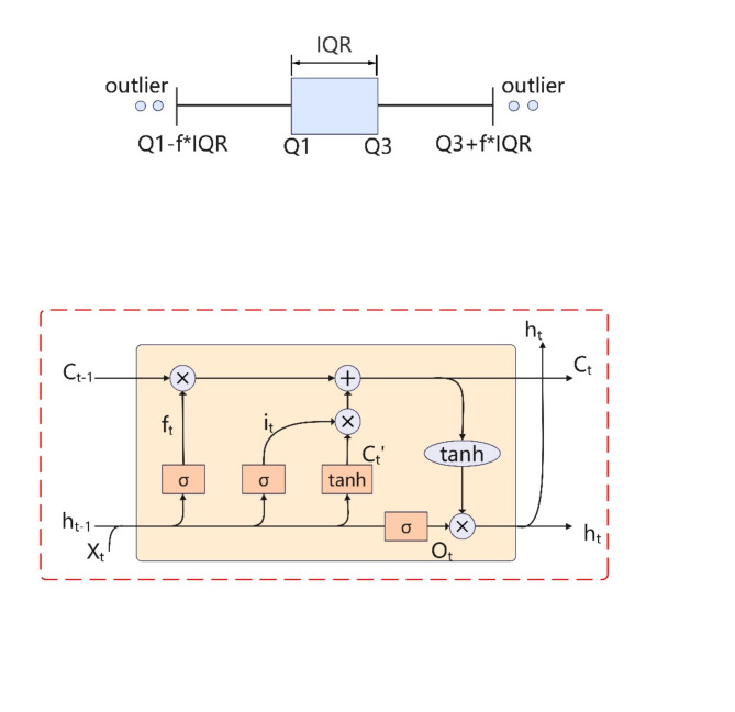
In this study, we collected over 18,000 drilling data points from several blocks in the Dagang oil field in China, including drill bit types (DT), drill bit size (DS), initial depth (ID), terminal depth (TD), drilling depth (DD), bit pressure drop (BP), hydraulic percussion (HP), spouting velocity (SV), specific hydraulic horsepower (SH), WOB, RPM, Q, MD, pump pressure (PP), and annulus dynamic pressure lost (DPS). First, we removed all irregular data and null values. For completely duplicate data, only one data record was retained.For the outliers encountered, we used the Interquartile Range (IQR) method for detection and removal¹⁷. The method allows for a comprehensive understanding of the data distribution, enabling the reasonable removal of outliers.

Mixed sampling

Due to the imbalanced distribution of ROP data, as shown in Fig. 1,the proportion of data in the 20–40 interval is significantly lower compared to the 0–20 interval, which can negatively impact model training performance. Therefore, it is necessary to perform sampling on the data. Employing only undersampling could result in a substantial reduction of data in the 0–20 interval, whereas using only oversampling might lead to an excessive amount of generated data in the 20–40 interval^18,19. Hence, this study opted for a combined approach, utilizing both undersampling and oversampling techniques²⁰, We performed random undersampling on the data in the 20–40 ROP range to reduce the sample size to 70% of its original volume. For the 0–20 ROP range, we performed random oversampling to increase the sample size to twice its original volume. We then combined the results of these two sampling methods. This approach ensures the authenticity of the data while making the data distribution more uniform. This method was derived from our preliminary research, and in the discussion section, we will explore the impact of different sampling methods on model performance.

Fig. 1.

Rate of penetration mixed sampling.

Filtering

To make the data smoother, remove more spurious noise, and allow the model to fully learn the data features, we chose to use Daubechies 4 (db4) wavelets for data smoothing. This choice was made because db4 has good smoothness and compact support when processing time series data. We set the decomposition level to 2, which is a compromise that allows us to retain the main signal features while effectively removing high-frequency noise. We used the standard deviation as the threshold because it reflects data volatility and is suitable as a denoising threshold, and we applied a nonlinear thresholding method. The principle is that after wavelet transformation, the energy of useful signals concentrates on a few wavelet coefficients, while white noise remains dispersed among many wavelet coefficients in the wavelet domain. Therefore, the wavelet coefficients of useful signals must be greater than those of the dispersed, low-amplitude noise. As a result, useful signals and noise can be separated in terms of spectral amplitude.

1

is the wavelet basis function, is the translation parameter, and is the transformed wavelet coefficient. The high-frequency information is contained in the detail coefficients, while the low-frequency information is contained in the approximation coefficients²¹.

Final data

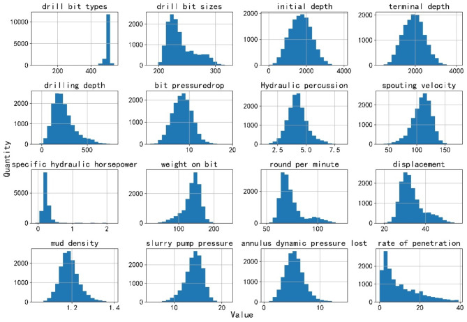
After data preprocessing, a total of 15,467 drilling data points were obtained. The specific distribution is illustrated in Fig. 2.

Fig. 2.

Data statistics.

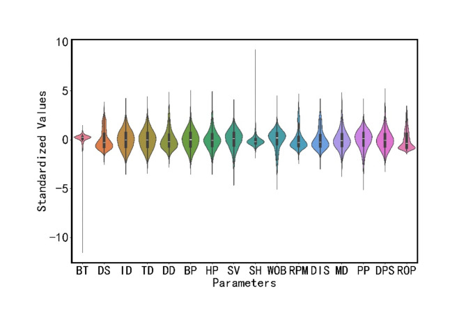
To more intuitively observe the distribution of each type of data, Fig. 3 displays violin plots of the standardized parameters. From the figure, the quartile range and density distribution of the data can be observed. It can be seen that the final data is consistent with the actual construction conditions, and its distribution is similar to that of a normal distribution, meeting the requirements for machine learning training.

Fig. 3.

Data distribution.

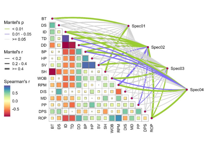
Next, the data underwent Spearman correlation analysis and Mantel test, forming a network correlation heatmap. First, the Spearman correlation analysis was used to measure the correlation between two variables, making it suitable for data with nonlinear relationships. Secondly, we used the Mantel test to assess the correlation between different parameter groups. We categorized the parameters into four groups: drilling tool parameters (BT, DS), well depth-related parameters (ID, TD, DD), other operational parameters (BP, HP, SV, SH, WOB, RPM, Q, MD, PP, DPS), and ROP, labeling them as Spec01 to Spec04 respectively. We then analyzed each parameter within these groups individually. Mantel correlation coefficient (Mantel’s ) is used to measure the correlation level between two distance matrices. When the value is close to, it indicates a high positive linear correlation between the two distance matrices; when thevalue is close to , it indicates a high negative linear correlation between them. Mantel’sis used to assess whether the observed Mantel’svalue has statistical significance. If theis smaller, it indicates that Mantel’svalue is less likely to be a random event, and the correlation between the two groups of distance matrices has statistical significance. If theis larger, it means that Mantel’svalue is more likely to be a random event, and the correlation between the two groups of distance matrices lacks statistical significance. The final results are shown in Fig. 4. It is evident that DD, WOB, and RPM have a strong positive correlation with the ROP. Other parameters also have some correlation with the ROP, and therefore, BT, DS, ID, TD, DD, BP, HP, SV, SH, WOB, RPM, Q, MD, PP, and DPS can all be used as input parameters to predict the ROP.

Fig. 4.

Network correlation heatmap.

We divided the dataset for each well according to the time sequence, extracting data from the early, middle, and late stages of the time series to form the validation set, resulting in a training-to-validation ratio of 8:2. This approach not only ensures that the model learns the diverse characteristics of the drilling data but also preserves the time series features of the dataset. Additionally, we selected drilling data from different sources than those used in the training and validation sets as the test set to evaluate the model’s actual predictive capability.

Method

Physical equation

Physical models are based on engineering principles and physical laws of the drilling process, directly describing the relationship between ROP and various influencing factors. They possess good interpretability, help to understand the relationship between ROP and influencing factors, and allow for parameter adjustments based on actual drilling conditions. In contrast to physical models, machine learning models can make full use of a large amount of drilling data for prediction, but machine learning has high requirements for data quality, and the data collected in practice may contain some noise. Therefore, by combining physical models with machine learning models, we can obtain a model with improved prediction capabilities.

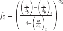
There are many types of traditional ROP prediction equations, each derived from empirical formulas obtained through extensive experiments based on downhole environments and parameters. A typical model is the B-Y equation. The expression for the B-Y equation is⁴:

2

3

4

5

6

7

8

9

10

In these equations,epresents the vertical depth,is the equivalent mud weight of the pore pressure, is the pore pressure at the drilling start point, s the equivalent circulating density,is the influencing factor,is the RPM,is the wear length of the drill bit cutting teeth,is the WOB, is the drilling fluid density,is the flow rate,stands for apparent viscosity,is the diameter of the drill bit,represents the formation strength effects,andrepresent compaction effects,is the overbalance effect,andrepresent the effects of RPM and WOB ,is the effect of tooth wear,is the hydraulic effect of the drill bit. Constants-need to be determined based on the actual construction environment²².

The B-Y equation is comprehensive and has good predictive capabilities. However, it also has drawbacks, as it involves a large number of parameters. In some downhole environments, it may not be possible to collect all these parameters, rendering the equation inapplicable.

Similarly, Maurer proposed a ROP prediction equation, with the expression as follows³ :

11

represents the drillability constant, is the RPM, is the weight on bit, is the diameter of the drill bit, is the rock’s compressive strength.

Bingham improved Maurer’s equation by reducing the number of parameters while maintaining prediction accuracy, allowing for more convenient practical application. The expression for Bingham’s equation is as follows²³:

12

represents the drillability constant, is the RPM, is the weight on bit, is the diameter of the drill bit, is the weight coefficient measured in the experiment.

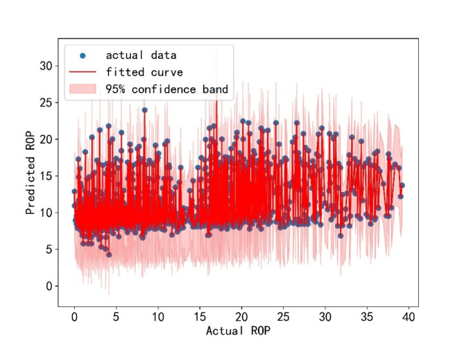
In this study, we chose Bingham’s equation and combined it with the optimized machine learning model to form a hybrid model. The specific implementation is as follows: First, we randomly extracted 10% of the data from the dataset and used it in the Bingham equation. We applied the least squares method to fit the extracted data. Utilizing the least squares method allows for the easy determination of unknown data while keeping the error between the obtained data and the actual data to a minimum^24,25.Ultimately, the drillability constant =0.125 and the weight coefficient =-0.196 were obtained, The fitted curve is shown in Fig. 5.

Fig. 5.

Least squares fitting curve.

The resulting Bingham equation is:

13

By applying the equation to the dataset, we can predict the ROP. Then, the predicted ROP is used as a new feature, combined with other parameters, and input into the machine learning model for training. This process yields the final ROP, effectively combining the Bingham equation with the machine learning model.

Machine learning model

Since drilling data is sequentially recorded and exhibits strong temporal characteristics, this study chose the Long Short-Term Memory (LSTM) network as the base model. Compared to convolutional neural networks and ensemble models such as random forests, LSTM has a stronger analysis capability when handling time series and sequence data. In contrast to traditional recurrent neural networks, LSTM effectively solves the long sequence problem and overcomes the issues of vanishing and exploding gradients by introducing concepts of memory cells, forget gates, input gates, and output gates²⁶. The structure of the component units is depicted in Fig. 6.

Fig. 6.

LSTM basic architecture diagram.

Memory cells are responsible for storing important information and passing it on to subsequent network layers. Forget gates regulate the amount of information from the previous time step’s cell state that remains relevant for the current time step’s cell state, essentially deciding which information should be discarded. This gate takesand as inputs, after passing through the sigmoid layer, outputs within the [0,1] interval, which is then pointwise multiplied by the numbers in the cell state .The expression is as follows²⁷:

14

In this expression, represents the sigmoid activation function, is the weight coefficient, andis the bias coefficient.

The input gate determines how much of the input at the current time step is included in the current cell state, comprising a sigmoid layer and a tanh layer. The tanh layer generates a new cell state value vector , which is incorporated into the state, expressed as follows:

15

16

Where and ​ represent weight coefficients, and and ​ are bias coefficients.

The output gate regulates the extent to which the current time step’s cell state is emitted. By utilizing the sigmoid function, the cell state is passed forward. The expression is as follows:

17

18

​ is obtained from and The calculation method for is the same as for ​ and .

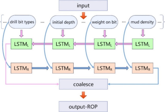
The original LSTM is a unidirectional structure, only retaining past data without taking into account future data. Considering the large amount and complexity of drilling data, this study improved the model by implementing a BiLSTM²⁸, This allows the model to focus on both past and future data simultaneously, leading to a better understanding of data features. The operational schematic of the model is shown in Fig. 7.

Fig. 7.

BiLSTM schematic diagram.

Incorporating attention mechanism

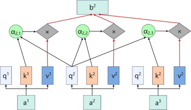
Neural networks receive inputs consisting of many vectors of varying sizes. These vectors have some relationships between them, but during actual training, it can be challenging to fully learn the relationships between these inputs, leading to suboptimal model performance. As illustrated in Fig. 8, the self-attention mechanism can address this issue by capturing the relationships among the input features²⁹.

Fig. 8.

Self-Attention mechanism architecture diagram.

In this mechanism, represents the query vector, represents the key vector, and represents the value vector. denotes the attention score. It can be seen that the final output takes into account not only the properties of but also the relationships among , ,and other inputs. The expression is as follows:

19

Where is a scaling factor, and represents the transpose of the matrix.

Although the LSTM structure solves the long sequence problem to some extent, it may still encounter vanishing or exploding gradients when dealing with large amounts of data or overly complex issues, gradually neglecting earlier input features. In contrast, the self-attention mechanism effectively considers earlier inputs, handles long sequence data more efficiently, captures global dependencies, and reduces information loss. The self-attention mechanism can adjust attention weights based on the input data, allowing it to flexibly focus on different parts of the sequence. This mechanism enables the model to more effectively utilize important information, thereby improving the model’s accuracy. Moreover, unlike LSTM, which processes input and output sequentially, the self-attention mechanism employs parallel computation, allowing for simultaneous input and output processing. By incorporating the structure shown in Fig. 8 into each submodule of Fig. 7, the integration of BiLSTM and the self-attention mechanism can be achieved. This approach not only improves computational efficiency but also ensures training accuracy. Therefore, combining the bidirectional LSTM model with the self-attention mechanism can overcome the limitations of using LSTM alone, further enhancing the model’s performance^30,31.

Optimizing regularization and learning rate

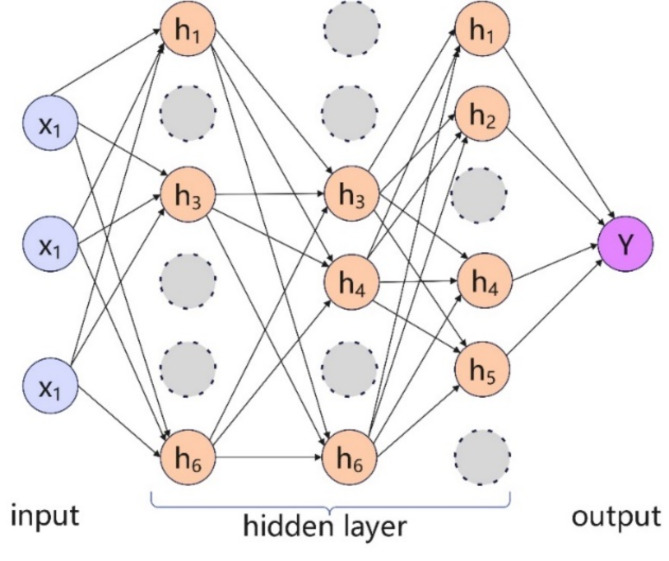
In the experiments, we found that as the number of training iterations increased, the model was prone to overfitting. Traditional regularization methods only used one approach, which had certain drawbacks. If the regularization coefficient was set too small, the regularization effect was not obvious, and the model would still be overfitting. If the coefficient was set too large, it would lead to poor training results. To address this issue, this study introduced both Dropout and LASSO regression (L1 regularization) simultaneously³², and used optimization algorithms to obtain the optimal combination coefficients for the two methods. Figure 9 illustrates the workflow of Dropout. The main idea of Dropout is to randomly drop a portion of neurons so that the network does not overly rely on other neurons, thus enhancing its robustness. This way, the network model can better adapt to new data. L1 regularization can be considered as a penalty term in the loss function. It restricts some parameters in the loss function, allowing the parameters to take values within a certain range. The expression for L1 regularization is³³:

20

Fig. 9.

Dropout neuron schematic diagram.

represents the original loss function, and denotes the L1 regularization term. L1 regularization is the sum of the absolute values of the elements in the weight vector, which serves to increase the loss value.

The learning rate represents the magnitude of change in network parameters during each iteration. In machine learning training, a larger initial learning rate is needed for the model to quickly find the optimal solution area. As the number of training iterations increases, the model requires a smaller learning rate for adjustments³⁴.Therefore, this study chose to adjust the learning rate at equal intervals. After every 5 iterations, the learning rate is decayed to 90% of its previous value.

Optimization algorithm

Dung beetle optimizer

Due to the numerous improvements made to the base model as discussed earlier, the model complexity has increased accordingly, making it more difficult to set hyperparameters. Therefore, this study chose to use an optimization algorithm to automatically search for the best parameters, thereby improving model performance³⁵. The Dung Beetle Optimizer (DBO) is a relatively novel swarm intelligence optimization algorithm with advantages such as strong search capability and rapid convergence speed, allowing it to address complex problems. DBO primarily updates positions based on the characteristics of dung beetle ball rolling, dancing, breeding, foraging, and thieving behaviors. The original author of the algorithm believes that light sources can affect the dung beetle’s path, with the ball rolling formula as follows³⁶ :

21

represents the current iteration, represents the positional data of dung beetleduring iteration,represents the deflection coefficient, denotes the coefficient of light intensity,stands for the natural coefficient, simulates the variation in light intensity, and symbolizes the global worst position.

When the dung beetle encounters obstacles while rolling the ball, it performs a dancing behavior to reorient itself. The dancing behavior is modeled as a tangent function, but only considers values within theinterval. The formula is as follows:

22

To search for the optimization region, a boundary selection strategy is employed, which simulates the egg-laying area of the dung beetle. The expression for this is as follows:

23

represents the local optimal position,andindicating the boundaries of the egg-laying region, respectively, whileandrepresent the minimum and maximum limits of the optimization problem. , and represent the maximum number of iterations and the current number of iterations, respectively.

Once the egg-laying area is determined, the dung beetle proceeds to lay eggs. The expression as follows:

24

represents the position information of egg-ball at iteration ,andare random vectors with dimensions matching the optimization problem.

Once the eggs hatch, the young dung beetles begin foraging. The boundary of the optimal foraging area is expressed the same way as the boundary for the egg-laying area. In the final stage, thieving behavior occurs, where some dung beetles steal the optimal food sources. The thief’s positional information is provided below:

25

represents the position information of thief at iteration is a random vector with a normally distributed magnitude, andis a constant.

In this study, we choose the DBO to optimize the aforementioned model. During the optimization process, due to the complexity of the model and the large number of parameters, using many dung beetle particles for extensive searches would significantly increase the optimization time. Thus, we can only choose a relatively small number of particles and iterations. Under this premise, it is crucial to ensure a uniform initial population distribution, strong global exploration and local exploitation capabilities, and to avoid getting trapped in local optima. Therefore, based on the practical application problem, we made a series of improvements to the DBO, making it more suitable for this optimization task.

Sobol sequence for Initializing Population positions

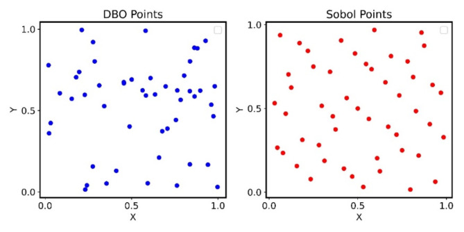
The Sobol sequence is a low-discrepancy deterministic sequence. Compared to traditional random number generators, the Sobol sequence has better uniform distribution properties, providing faster convergence speed using the same number of points³⁷, Fig. 10 illustrates the particle distribution when using the Sobol sequence for initializing population positions.

Fig. 10.

Comparison diagram of random distribution and sobol sequence initialization.

Integrating golden sine algorithm

Golden Sine Algorithm is a novel meta-heuristic algorithm proposed by Tanyildizi and colleagues in 2017. The algorithm utilizes the sine function to find optimal values while introducing the golden ratio to narrow the search space and increase search speed. The expression for the Golden Sine Algorithm is as follows³⁸ :

26

represents the next position of individual, the value of is a randomly generated number within the interval, whileis another randomly generated number within the interval,denotes the best location for individualat iteration ,and are the golden ratio coefficients.

Considering the large number of model parameters and the lengthy optimization time, to accelerate the search for the optimal solution, the Golden Sine Algorithm is integrated into the DBO’s particle position update while using the original DBO as well.

Integrating dynamic decreasing factor

In the experiments, we found that the previous optimization algorithm could eventually find a relatively optimal solution. However, by examining the particle search trajectory, we discovered that it was still prone to getting trapped in local optima. Therefore, we integrated a decreasing factor into the particle position update. Specifically, we generated two random vectors within the optimization range, calculated their difference, and multiplied the result by a dynamic factor, which was then incorporated into the original position update function. By introducing the dynamic decreasing factor, we can further prevent entrapment in local optima. The decreasing factor size can be adjusted through the dynamic factor, which diminishes as the number of iterations increases. The expression for the dynamic decreasing factor is as follows:

27

28

29

is the random vector,andrepresent the maximum and minimum values of the parameters,is a randomly generated vector with the number of elements equal to the number of parameters to be optimized. The element values are randomly sampled from theinterval. is the coefficient of the decreasing factor, which can be custom-defined,is the dynamic factor,is the current iteration number, is the maximum number of iterations, is the result of subtraction.

In this study, we choose to optimize the hidden layer, initial learning rate, batch size, the number of network layers, L1 regularization coefficient, and Dropout coefficient for the BILSTM-SA model. Hidden layers are hierarchical structures situated between the input and output layers, used for feature extraction. Increasing the number of hidden layers can enhance the network’s complexity and fitting capability, but too many layers can increase the risk of overfitting and also raise training time and computational costs. The learning rate determines the extent of parameter updates during each iteration; if set too high, the model may oscillate and fail to converge, while if set too low, the convergence speed may be too slow. Therefore, selecting an appropriate initial learning rate is crucial for the entire training process. Batch size refers to the number of samples the model processes during each iteration; larger batch sizes can reduce oscillations during gradient updates, making the model more stable in convergence but also consuming more computational resources. The number of network layers refers to the layers of BiLSTM. Regularization methods have been detailed in the previous section.These parameters are crucial hyperparameters in machine learning training. If set manually, they can only be determined through trial and error, which is inefficient and inaccurate. Many previous models for ROP prediction did not use optimization algorithms for hyperparameter tuning, resulting in suboptimal performance. Therefore, it is necessary to use optimization algorithms to optimize these hyperparameters.

End-to-end BiLSTM-SA-IDBO

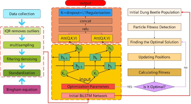
In traditional machine learning, it is necessary to manually divide many submodules between a task’s input and output, splitting it into several stages. Each module and stage is learned separately before being assembled. In contrast, end-to-end machine learning treats the process from input to output as a unified model, directly optimizing the overall objective of the task. This approach is more meaningful for practical applications and facilitates model optimization at later stages³⁹. In this study, we propose an end-to-end BiLSTM-SA-IDBO model, which integrates the improved Dung Beetle Optimizer algorithm and the self-attention mechanism into the BiLSTM model, and incorporates a physics-based model at the data level. The final model’s workflow diagram is shown in Fig. 11. The overall architecture of the model includes an input layer, BiLSTM layers, self-attention layers, and an output layer. The input layer receives the drilling data, which is preprocessed and then fed into the BiLSTM layers. The BiLSTM, combined with the self-attention mechanism, processes the time series data and extracts features. Finally, the output layer provides the prediction results. In practical applications, all these modules are integrated into a single model, where inputting the data at the input end will directly yield the predicted ROP.

Fig. 11.

BiLSTM-SA-IDBO network architecture diagram.

Evaluation metrics

We selected commonly used evaluation metrics for regression tasks⁴⁰. The first metric is the Root Mean Square Error (RMSE), which calculates the square root of the sum of the squared differences between the predicted values and the true values. The expression for RMSE is:

30

The second metric is the Coefficient of Determination, or R-square, which indicates the degree to which the model fits the data. The expression for R-square is as follows:

31

The third is Mean Absolute Error (MAE), which represents the average error between the predicted values and the actual values.

32

represents the actual value,represents the predicted value,represents the average of the actual values.

Results

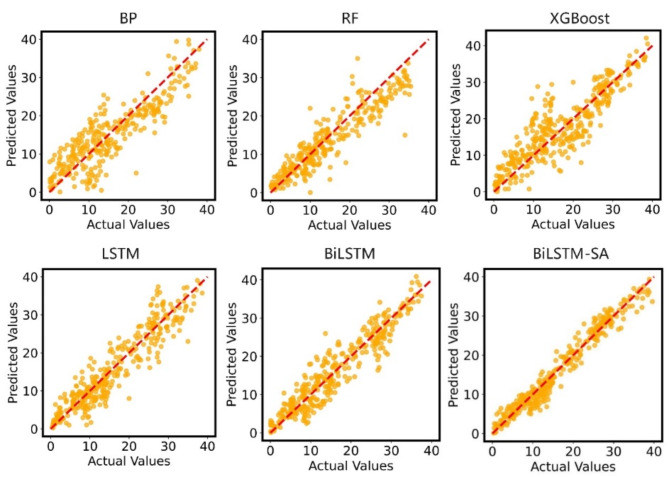
Before obtaining the final results, we conducted ablation studies using other models, including Backpropagation Neural Network (BP), RF, XGBoost, LSTM, BiLSTM, and BiLSTM-SA. We also used the Bingham equation for testing. The final test results are shown in Table 2. After each training is completed, we randomly selected 300 data points for testing. Figure 12 displays the fitting effect of the model.

Table 2.

Comparison of model performances without bingham equation.

Model	Epoch	Initial learning rate	RMSE	R 2	MAE
BP	100	0.01	1.35	0.311	1.16
RF	100	/	1.01	0.35	0.834
XGBoost	100	0.01	0.901	0.435	0.78
LSTM	100	0.01	0.7	0.594	0.572
BiLSTM	100	0.01	0.61	0.66	0.509
BiLSTM-SA	100	0.01	0.41	0.698	0.335
Bingham Equation	/	/	5.17	0.138	4.447

Fig. 12.

Fitting performance of different models without bingham equation.

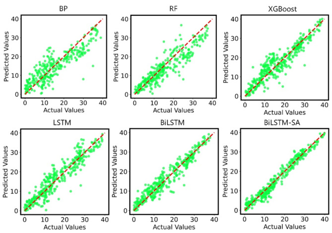
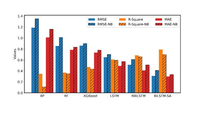
To examine the impact of incorporating the Bingham equation on the models, we fused the Bingham equation into each of the aforementioned models. Then, keeping other parameters constant, we trained and tested each model again. As displayed in Table 3, the ultimate findings are presented, and the fitting effect is displayed in Fig. 13. Figure 14 exhibits the comparison of the six models before and after fusing the Bingham equation.

Table 3.

Comparison of different model performances with bingham equation.

Model	Epoch	Initial Learning Rate	RMSE	R 2	MAE
BP	100	0.01	1.19	0.347	1.01
RF	100	/	0.856	0.370	0.786
XGBoost	100	0.01	0.86	0.471	0.735
LSTM	100	0.01	0.650	0.610	0.492
BiLSTM	100	0.01	0.512	0.686	0.410
BiLSTM-SA	100	0.01	0.309	0.790	0.298

Fig. 13.

Fitting performance of different models without bingham equation.

Fig. 14.

Performance comparison of six models before and after incorporating the Bingham equation, where NB represents models without Bingham equation.

Based on the evaluation metrics and fitting plots, we observe the following: First, the performance of machine learning models combined with the Bingham equation is superior and significantly surpasses the pure Bingham equation. Second, the BiLSTM-SA model has the best fitting effect. Next, we will use different optimization algorithms to optimize this model and improve its performance. We performed optimization experiments using DBO, IDBO, and Particle Swarm Optimization (PSO). For all three optimization algorithms, we set 30 particles and 30 iterations. The parameters to optimize and their respective ranges are are shown in Table 4.

Table 4.

Parameters to be optimized and their ranges.

Parameter	Minimum value	Maximum value
Hidden size	32	256
Learning rate	0.0001	0.1
Batch size	64	512
Num layers	1	4
L1 Regularization	0.0001	0.1
Dropout rate	0.1	0.8

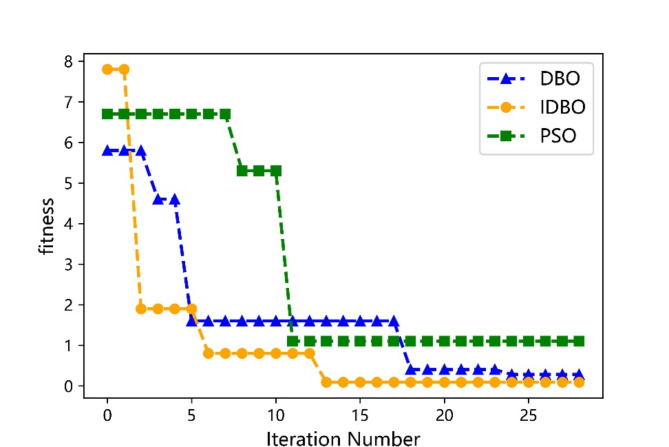
We recorded the fitness curves for the three optimization algorithms, as shown in Fig. 15, and documented the total optimization time for each algorithm: PSO took 3 h and 13 min, DBO took 2 h and 44 min, and IDBO took 2 h and 57 min. The results indicate that PSO is the slowest, while DBO is the fastest, but the time difference with IDBO is not significant. Given that the current application scenario does not require real-time optimization, IDBO is more suitable as it ensures accuracy.

Fig. 15.

The fitness curves for the three optimization algorithms.

To visualize the search trajectories of the three optimization algorithms more intuitively, we used PCA dimensionality reduction to reduce the optimization process of the six parameters from six dimensions to three dimensions. We then plotted search trajectory diagrams for each optimization algorithm in the three-dimensional space, as shown in Fig. 16.

Fig. 16.

Optimization algorithm search trajectory diagram.

The optimal combinations found by the three optimization algorithms are shown in Table 5. Then, we used the parameters in Table 5 to train the BiLSTM-SA model separately. The outcomes are presented in Table 6.

Table 5.

Optimization algorithm search results.

Optimization Algorithm	Hidden size	Learning rate	Batch Size	Num layers	L1 Regularization	Dropout rate
PSO	186	0.080	64	1	0.0004	0.34
DBO	200	0.045	64	4	0.0004	0.25
IDBO	256	0.090	512	3	0.0009	0.40

Table 6.

Results of BiLSTM trained with different parameters.

Optimization Algorithm	Model	Epoch	RMSE	R 2	MAE
PSO	BiLSTM-SA	100	0.310	0.784	0.234
DBO	BiLSTM-SA	100	0.118	0.878	0.107
IDBO	BiLSTM-SA	100	0.065	0.963	0.05

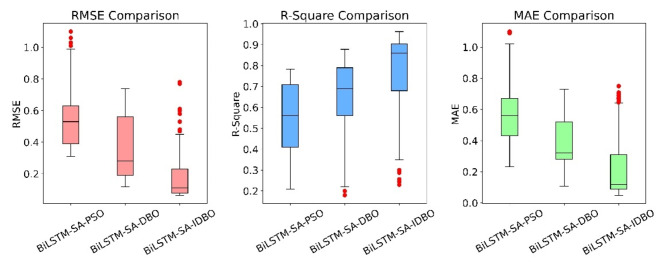
Next, we recorded the metrics for each epoch during the training process, as shown in Fig. 17. It can be observed that the overall performance of BiLSTM-SA-IDBO is better.

Fig. 17.

Performance metrics statistics for the three optimization models.

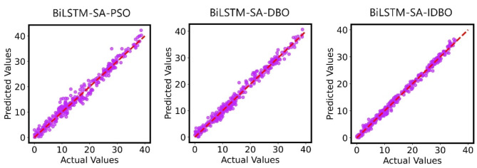
To further examine the prediction performance, we also randomly selected 300 data points and tested them using BiLSTM-SA-PSO, BiLSTM-SA-DBO, and BiLSTM-SA-IDBO models. Figure 18 displays the fitting effect and shows that the predictive performance of the BiLSTM-SA model improved after optimization with each algorithm, especially for the BiLSTM-SA-IDBO which had the best performance.

Fig. 18.

Fitting results of BiLSTM optimized by three different optimization algorithms.

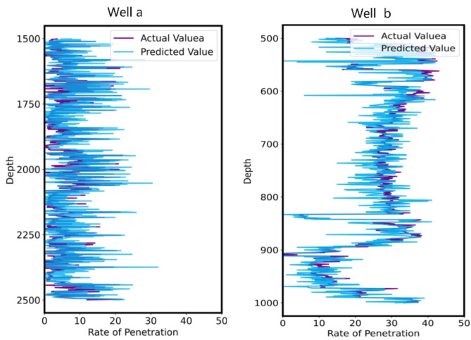
Based on the actual needs of the oil field, the model was applied to the construction site for prediction. Figure 19 shows some of the prediction results, indicating good model accuracy.

Fig. 19.

On-site actual prediction performance.

Discussion

The above research results indicate that the BiLSTM-SA-IDBO model shows significant improvements in various evaluation metrics compared to other models. These metric enhancements not only demonstrate the superior performance of the model in the task of predicting ROP but also highlight its practical significance in real-world applications. The optimization of RMSE significantly reduces the gap between predicted and actual values, improving prediction accuracy and reducing the likelihood of large errors, which is crucial in high-risk, high-cost fields such as oil drilling. The optimization of R² enhances the model’s fitting capability and improves data utilization. The improvement in MAE indicates that the model’s prediction errors are more stable, enhancing the reliability of the model in practical applications. Overall, these improvements in evaluation metrics lead to better overall performance of the model, which can help drilling design engineers better allocate and utilize drilling resources, avoid resource wastage, and optimize drilling parameters, thereby improving drilling efficiency and reducing costs.

However, some aspects require further discussion and supplementation. In this study, based on our research, we initially selected a mixed sampling for data sampling to further verify its reliability. We performed oversampling, undersampling, mixed sampling, and no sampling on the data. Then, we trained the BiLSTM-SA model using the data obtained from these four sampling methods in the same manner. The results, as shown in Table 7, indicate that mixed sampling performed the best.

Table 7.

The final results of different sampling methods.

Sampling method	RMSE	R 2	MAE
No sampling	1.315	0.314	1.020
Over sampling	0.63	0.527	0.430
Under sampling	1.138	0.394	0.824
Mixed sampling	0.309	0.790	0.298

In conclusion, in oil drilling and other fields, imbalanced data distribution is a common issue, and selecting an appropriate sampling strategy is crucial. Mixed sampling can be considered the preferred solution to enhance model performance and generalization capability. No sampling maintains the original state of the data, oversampling may lead to overfitting, and undersampling may result in data loss. Mixed sampling effectively balances the data while reducing the drawbacks of oversampling and undersampling, thereby improving model predictive performance.

Additionally, this paper proposes IDBO, which achieves uniform population distribution through Sobol sequences and integrates the Golden Sine algorithm and dynamic subtraction factors to enhance overall optimization capability. We infer that this method has significant potential for application in similar optimization tasks. Our dataset is relatively large and includes many model parameters that need optimization; therefore, IDBO remains applicable in similar tasks. However, model performance is highly dependent on the choice of algorithm and dataset, and general conclusions can only be drawn through practical application.

A current notable drawback is the long optimization time, which makes real-time optimization unfeasible. Especially in the future, we plan to achieve real-time optimization of drilling parameters based on precise ROP prediction, thereby providing greater practical value for drilling operations. However, without an algorithm capable of real-time optimization, this goal will be difficult to achieve. This necessitates adjustments in our optimization strategy, such as improving the optimization algorithm or conducting preliminary experiments to reduce the number and range of parameters needing optimization, thereby significantly enhancing optimization efficiency.

Despite the outstanding performance of the BiLSTM-SA-IDBO model in predicting ROP, the diversity of oilfields and drilling conditions remains a significant challenge in practical applications. To address this issue, future research will explore the application of transfer learning to enhance the model’s robustness and generalization capabilities. Transfer learning is a method that applies a pre-trained model to new domains or tasks, effectively reducing training time and improving the model’s performance in new environments⁴¹. In the field of oil drilling, transfer learning can help quickly adapt a model trained in one oilfield to other oilfields, thereby reducing the data and time required for retraining. In future work, we plan to develop a multi-domain adaptive model that utilizes transfer learning techniques to maintain high accuracy and reliability under different drilling conditions.

Conclusion

This study proposes an end-to-end ROP prediction model based on a BiLSTM integrated with a Self-Attention mechanism and an Improved Dung Beetle Optimization. Experimental results indicate that this model performs excellently in predicting ROP, with an RMSE of 0.065, an R² of 0.963, and an MAE of 0.05. These evaluation metrics are significantly better than those of other models. Additionally, these results demonstrate the effectiveness of combining physical models with data-driven models. The main contributions are as follows:

(1)We collected data from multiple wells in the Dagang Oilfield, enhanced data quality through mixed sampling and wavelet filtering techniques, and integrated the Bingham equation into the BiLSTM, achieving a combination of physical models and data-driven models.

(2)We introduced a self-attention mechanism into the BiLSTM, strengthening the model’s ability to learn important features, thereby improving prediction accuracy and the model’s generalization capability.

(3)We employed the improved IDBO, integrating Sobol sequences, the Golden Sine algorithm, and dynamic subtraction factors to enhance the efficiency and effectiveness of model parameter optimization. Comparisons show that while the total optimization time of IDBO is slightly longer than DBO, the performance of the BiLSTM-SA model optimized by IDBO is superior, with RMSE and MAE reduced by 44.9% and 53.2%, respectively, and R² increased by 9.68%.

Despite the model’s outstanding performance in predicting ROP, there are still some limitations:

(1)The collected data needs to be further diversified to enhance the model’s generalization and effectiveness.

(2)The optimization algorithm has a long optimization time, making real-time optimization unfeasible.

(3)The current model primarily targets training and prediction on offline data, lacking the capability to handle real-time data.

In the future, we plan to collect a broader range of data from the field for model training. We will also further adjust the optimization algorithm structure or conduct extensive preliminary experiments to reduce the computational load of on-site optimization, ensuring both accuracy and efficiency. Additionally, we will focus on building online prediction models and transfer learning models to significantly enhance the practical value of the models.

Author contributions

M.X. designed the study, coded the software, and wrote the manuscript; S.Z. provided ideas and thoughts; W.L. revised; R.C. and L.W. collected the sample dataset; H.Z. and G.W. conducted on-site testing.

Data availability

The datasets analysed during the current study are not publicly available due to data privacy, but are available from the corresponding author on reasonable request.

Declarations

Competing interests

The authors declare no competing interests.

References

- 1.Shaygan, K. & Jamshidi, S. Prediction of rate of penetration in directional drilling using data mining techniques. Geoenerg Sci. Eng. 221, 111293 (2023). [Google Scholar]
- 2.Jiao, S. et al. Hybrid physics-machine learning models for predicting rate of penetration in the Halahatang oil field, Tarim Basin. Sci. Rep. 14 10.1038/s41598-024-56640-y (2024). [DOI] [PMC free article] [PubMed]
- 3.Maurer, W. The perfect-cleaning theory of rotary drilling. J. Pet. Technol. 14, 1270–1274 (1962). [Google Scholar]
- 4.Bourgoyne, A. T. Jr & Young, F. Jr A multiple regression approach to optimal drilling and abnormal pressure detection. Soc. Pet. Eng. J. 14, 371–384 (1974). [Google Scholar]
- 5.Warren, T. Penetration-rate performance of roller-cone bits. SPE Drill. Eng. 2, 9–18 (1987). [Google Scholar]
- 6.Xiang, X., Li, X., Zhang, Y. & Hu, J. A short-term forecasting method for photovoltaic power generation based on the TCN-ECANet-GRU hybrid model. Sci. Rep. 14 10.1038/s41598-024-56751-6 (2024). [DOI] [PMC free article] [PubMed]
- 7.Li, W. et al. Application of a hybrid algorithm of LSTM and Transformer based on random search optimization for improving rainfall-runoff simulation. Sci. Rep. 14, 11184–11184. 10.1038/s41598-024-62127-7 (2024). [DOI] [PMC free article] [PubMed] [Google Scholar]
- 8.Hegde, C. & Gray, K. Use of machine learning and data analytics to increase drilling efficiency for nearby wells. J. Nat. Gas Sci. Eng. 40, 327–335 (2017). [Google Scholar]
- 9.Soares, C. & Gray, K. Real-time predictive capabilities of analytical and machine learning rate of penetration (ROP) models. J. Pet. Sci. Eng. 172, 934–959 (2019). [Google Scholar]
- 10.Mehrad, M., Bajolvand, M., Ramezanzadeh, A. & Neycharan, J. G. Developing a new rigorous drilling rate prediction model using a machine learning technique. J. Pet. Sci. Eng. 192, 107338 (2020). [Google Scholar]
- 11.Liu, N. P., Gao, H., Zhao, Z., Hu, Y. L. & Duan, L. C. A stacked generalization ensemble model for optimization and prediction of the gas well rate of penetration: a case study in Xinjiang. J. Pet. Explor. Prod. Technol. 12, 1595–1608. 10.1007/s13202-021-01402-z (2022). [Google Scholar]
- 12.Hashemizadeh, A., Bahonar, E., Chahardowli, M., Kheirollahi, H. & Simjoo, M. Analysis of rate of penetration prediction in drilling using data-driven models based on weight on hook measurement. Earth Sci. Inf. 15, 2133–2153 (2022). [Google Scholar]
- 13.Yin, H., Zhao, X. & Li, Q. Research on adaptive prediction model of rate of penetration under dynamic formation conditions. Eng. Appl. Artif. Intell. 133, 108281. 10.1016/j.engappai.2024.108281 (2024). [Google Scholar]
- 14.Cheng, Z. et al. A sequential feature- based rate of penetration representation prediction method by attention long short- term Memory Network. SPE J. 29, 681–699 (2024). [Google Scholar]
- 15.Liu, W., Feng, J., Zhu, X. & Li, Z. Research on Drilling Rate Prediction Model based on Momentum adaptive learning rate PSO-BP neural network. Sci. Technol. Eng. 23, 10264–10272 (2023). [Google Scholar]
- 16.Tang, M., Wang, H., He, S., Zhang, G. & Kong, L. Research on Mechanical Drilling Rate Prediction based on PCA-BP Algorithm. Pet. Mach. 51, 23–31. 10.16082/j.cnki.issn.1001-4578.2023.10.004 (2023). [Google Scholar]
- 17.Walfish, S. A review of statistical outlier methods. Pharm. Technol. 30, 82 (2006). [Google Scholar]
- 18.Shelke, M. S., Deshmukh, P. R. & Shandilya, V. K. A review on imbalanced data handling using undersampling and oversampling technique. Int. J. Recent. Trends Eng. Res. 3, 444–449 (2017). [Google Scholar]
- 19.Liu, X. Y., Wu, J. & Zhou, Z. H. Exploratory undersampling for class-imbalance learning. IEEE Trans. Syst. Man. Cybern B Cybern. 39, 539–550 (2008). [DOI] [PubMed] [Google Scholar]
- 20.Jung, I., Ji, J., Cho, C. & EmSM Ensemble mixed sampling method for classifying imbalanced intrusion detection data. Electron. 11, 1346 (2022). [Google Scholar]
- 21.Daubechies, I. The wavelet transform, time-frequency localization and signal analysis. IEEE Trans. Inf. Theory. 36, 961–1005 (1990). [Google Scholar]
- 22.Ren, C., Huang, W. & Gao, D. Predicting rate of penetration of horizontal drilling by combining physical model with machine learning method in the China Jimusar Oil Field. SPE J. 28, 2713–2736 (2023). [Google Scholar]
- 23.Bingham, M. G. A new Approach to interpreting– rock Drillability (Petroleum Pub. Co., 1965).
- 24.Shi, H., Zhang, X., Gao, Y., Wang, S. & Ning, Y. Robust total least SquaresEstimation Method for Uncertain Linear Regression Model. Math. 11 10.3390/math11204354 (2023).
- 25.Levenberg, K. A method for the solution of certain non-linear problems in least squares. Q. Appl. Math. 2, 164–168 (1944). [Google Scholar]
- 26.Sang, S. & Li, L. A. Novel variant of LSTM Stock Prediction Method incorporating attention mechanism. Math. 12 10.3390/math12070945 (2024).
- 27.Zhang, M., Yuan, Z. M., Dai, S. S., Chen, M. L. & Incecik, A. LSTM RNN-based excitation force prediction for the real-time control of wave energy converters. Ocean. Eng. 306, 118023 (2024). [Google Scholar]
- 28.Zhang, H., Yang, G., Yu, H. L. & Zheng, Z. Kalman Filter-based CNN-BiLSTM-ATT Model for Traffic Flow Prediction. CMC-Comput Mater. Contin. 76, 1047–1063. 10.32604/cmc.2023.039274 (2023). [Google Scholar]
- 29.Yan, X., Gan, X., Wang, R. & Qin, T. Self-attention eidetic 3D-LSTM: video prediction models for traffic flow forecasting. Neurocomputing. 509, 167–176. 10.1016/j.neucom.2022.08.060 (2022). [Google Scholar]
- 30.Li, W., Qi, F., Tang, M. & Yu, Z. Bidirectional LSTM with self-attention mechanism and multi-channel features for sentiment classification. Neurocomputing. 387, 63–77 (2020). [Google Scholar]
- 31.Pan, S. et al. Oil well production prediction based on CNN-LSTM model with self-attention mechanism. Energy. 284, 128701. 10.1016/j.energy.2023.128701 (2023). [Google Scholar]
- 32.Meng, X., Xie, R., Jia, H. & Li, H. Identification of light oil in 2D NMR Spectra of tight sandstone reservoirs by using L1/L2 two-parameter regularization. Energy Fuels. 33, 10537–10546. 10.1021/acs.energyfuels.9b02114 (2019). [Google Scholar]
- 33.Zou, H. The adaptive lasso and its oracle properties. J. Am. Stat. Assoc. 101, 1418–1429 (2006). [Google Scholar]
- 34.Iiduka, H. Appropriate learning rates of adaptive learning rate optimization algorithms for training deep neural networks. IEEE Trans. Cybern. 52, 13250–13261. 10.1109/tcyb.2021.3107415 (2022). [DOI] [PubMed] [Google Scholar]
- 35.Zhou, Y., Wang, S., Xie, Y., Shen, X. & Fernandez, C. Remaining useful life prediction and state of health diagnosis for lithium-ion batteries based on improved grey wolf optimization algorithm-deep extreme learning machine algorithm. Energy. 285, 128761. 10.1016/j.energy.2023.128761 (2023). [Google Scholar]
- 36.Xue, J. & Shen, B. Dung beetle optimizer: a new meta-heuristic algorithm for global optimization. J. Supercomput. 79, 7305–7336 (2023). [Google Scholar]
- 37.Wu, Q., Xu, H. & Liu, M. Applying an Improved Dung Beetle Optimizer Algorithm to Network Traffic Identification. Comput. Mater. Contin. 78, 4091–4107 (2024).
- 38.Tanyildizi, E. & Demir, G. Golden sine algorithm: a Novel Math-inspired algorithm. Adv. Electr. Comput. Eng. 17, 71–78 (2017).
- 39.Liu, H., Liu, Z., Jia, W. & Lin, X. Remaining useful life prediction using a novel feature-attention-based end-to-end approach. IEEE Trans. Ind. Inf. 17, 1197–1207 (2020). [Google Scholar]
- 40.Afzal, S., Ziapour, B. M., Shokri, A., Shakibi, H. & Sobhani, B. Building energy consumption prediction using multilayer perceptron neural network-assisted models; comparison of different optimization algorithms. Energy. 282 10.1016/j.energy.2023.128446 (2023).
- 41.Zhuang, F. et al. A comprehensive survey on transfer learning. Proc. IEEE. 109, 43–76 (2020). [Google Scholar]
Associated Data
This section collects any data citations, data availability statements, or supplementary materials included in this article.
Data Availability Statement