

Abstract
Given the link between climatic factors on one hand, such as climate change and low frequency climate oscillation indices, and the occurrence and magnitude of heat waves on the other hand, and given the impact of heat waves on mortality, these climatic factors could provide some predictive skill for mortality. We propose a new model, the Mortality-Duration-Frequency (MDF) relationship, to relate the intensity of an extreme summer mortality event to its duration and frequency. The MDF model takes into account the non-stationarities observed in the mortality data through covariates by integrating information concerning climate change through the time trend and climate variability through climate oscillation indices. The proposed approach was applied to all-cause mortality data from 1983 to 2018 in the metropolitan regions of Quebec and Montreal in eastern Canada. In all cases, models introducing covariates lead to a substantial improvement in the goodness-of-fit in comparison to stationary models without covariates. Climate change signal is more important than climate variability signal in explaining maximum summer mortality. However, climate indices successfully explain a part of the interannual variability in the maximum summer mortality. Overall, the best models are obtained with the time trend and the North Atlantic Oscillation (NAO) used as covariates. No country has yet integrated teleconnection information in their heat-health watch and warning systems or adaptation plans. MDF modeling has the potential to be useful to public health managers for the planning and management of health services. It allows predicting future MDF curves for adaptive management using the values of the covariates.
Supplementary information
The online version contains supplementary material available at 10.1007/s00477-024-02813-0.
Keywords: Heat waves related mortality, Multivariate model, Adaptive management, Non-stationary models
Introduction
Heat waves, defined as extended periods of extreme temperature, are associated with excess daily mortality and morbidity (Bayentin et al. 2010; Masselot et al. 2018; Odame et al. 2018; Cheng et al. 2019; Vicedo-Cabrera et al. 2021). It is now well recognized that climate change caused by human activities has resulted in an increase in the frequency, duration and intensity of heat waves since the mid-20th century (Meehl and Tebaldi 2004; Coumou and Robinson 2013; Basha et al. 2017; Perkins-Kirkpatrick and Lewis 2020). According to global climate projections, these trends are expected to worsen in the future (Pachauri et al. 2014; Russo et al. 2014; Anderson et al. 2018) and are associated with increases in future heat wave-excess mortality (Guo et al. 2018). The recent observed heat waves, which have occurred in many regions with unprecedented adverse effects, have raised awareness among policy makers about this problem. These events have also led several countries to establish their own heat-health watch and warning systems (Casanueva et al. 2019). Although such warnings are useful on a short-term basis, it is also of interest to have an assessment of the expected burden of heat-related mortality on health systems, and in particular of its extremes, a few months in advance,
In addition to climate change, large-scale ocean-atmosphere interactions also have a significant impact on heat waves by modulating the decadal and interannual variability of land surface temperature at regional scales. For instance, in North America, extreme heat events have been linked to modes of climate variability in the Atlantic Ocean (the Atlantic Multidecadal Oscillation (AMO) (Mo et al. 2009), the North Atlantic Oscillation (NAO) and the Arctic Oscillation (AO) (Wettstein and Mearns 2002) and in the Pacific Ocean (the El Niño–Southern Oscillation (ENSO) (Seager et al. 2005), the Pacific Decadal Oscillation (PDO) (McCabe et al. 2004), the Pacific North American pattern (PNA) (Ning and Bradley 2016). Given the link between these low frequency climate oscillation indices and the occurrence and magnitude of heat waves, and given the well documented impact of heat waves on mortality, it would be logical to expect climate oscillation indices to provide some predictive skill of mortality and morbidity. These indices would prove valuable in anticipating the summer burden of heat-related mortality several months in advance. Our objective here, is therefore to propose a statistical approach to predict the intensity and frequency of the extremes of the warm season mortality using the information given by low frequency climate oscillation indices.
A heat wave is mainly characterized by its intensity and duration, both of major importance in terms of impact on populations. In this context, the Temperature-Duration-Frequency (TDF) relationship approach (Ouarda and Charron 2018) was recently proposed to jointly model the intensity, duration and frequency of heat events. It is proposed, in this work, to focus more closely on health by adapting the TDF concept to daily mortality data in a model denoted as Mortality-Duration-Frequency (MDF) curves, and to extend it to the nonstationary case by integrating information concerning climate change and climate variability. As summer extremes of mortality are largely driven by heat and are events that put health systems under intense pressure, models focusing on such extremes are of important interest to public health managers. Such a tool would be of interest to public health managers by providing predictions of the mortality burden due to climate, that is characterized jointly by the magnitude and duration of heatwaves associated with high mortality. The proposed approach differs from heat-health watch and alert systems because it is used to predict the risks associated with heatwaves and other climatic extremes during the coming summer season instead of triggering the alert on extreme heat days.
In the stationary formulation of TDF curves, it is assumed that the statistical characteristics (e.g. mean and variance) of the variable under study are invariant through time. However, excess mortality during summer is often caused by extreme temperatures for which it is known that characteristics change over time due to the influence of climate change or climate external forcings. Mortality time series are also subject to trends due to human factors such as infectious disease epidemics, demographic and exposure changes, improvements in medical practices and interventions, heat alert system implementations, physiological adaptations and responses, etc. The MDF model is thus adapted here to account for the non-stationarities observed in mortality data. For this, the parameters of the statistical distribution of the MDF model are made conditional on time-dependent covariates that explain mortality variability, such as the temporal trends, natural cycles, patterns of climatic oscillations, etc. (El Adlouni et al. 2007). The proposed MDF approach is applied in this study to observed daily mortality in the Montreal Metropolitan Community (MMC) and the Quebec Metropolitan Community (QMC), both in the province of Quebec (Canada).
The non-stationary model presented here would be particularly useful in the context of adaptive management (Andersson-Sköld et al. 2015; Vaughan et al. 2017). Such a management concept consists in a flexible strategy that adapts to changing social, environmental, climatic or economic conditions (Kingsborough et al. 2017). With the increasing risks associated to climate change, the influence of climate forcings or other factors not related to climate, management methods in the public health sector must be adapted to take into account the evolving conditions. In the present study, a covariate describing the long-term temporal trend (i.e. the year) and climate indices of oscillation patterns are used as covariates to predict MDF curves or surfaces. The approach is also expected to be useful for long-term projections of health impacts related to climate change. For this purpose, outputs of climate simulation models and the observed historical temporal trends can be efficiently used to predict future conditions. For climate indices, it is possible to obtain probabilistic climate forecasts for one or two decades into the future (McCabe et al. 2004; Lee and Ouarda 2011). For shorter-term forecasts (monthly to seasonal), values of appropriate low frequency climate oscillation indices prior to the period of extreme summer heat are commonly used as predictors for climate variables (White et al. 2014; Jacques-Coper et al. 2021; Laz et al. 2023). These indices are used as covariates in the nonstationary MDF model.
Methods
Nonstationary MDF relationship
The MDF approach is an adaptation of the TDF approach (Ouarda and Charron 2018) and the traditional rainfall Intensity-Duration-Frequency approach (IDF). For the developent of the original general IDF model the reader is referred to Koutsoyiannis et al. (1998), and for the development of the non-stationary IDF model the reader is referred to Ouarda et al. (2019a, b).
For the computation of the MDF relationships, the time series of the maximum average mortality (i.e. intensity) are derived from the daily observed deaths counts. For each year, the maximum average number of deaths for d (d = 1,…, D) consecutive days is extracted between June 1st and August 31st. The maximum average number of deaths for the year t is denoted by  ,
,  , where
  is the number of years with measurements and
  . Annual maximum of multi-day averages of daily mortality for selected durations during the summer season for both communities are illustrated in Fig. 1. Annual maximum of multi-day averages of daily mortality over all durations of 1 to 7 days during the summer for the MMC and QMC areas are respectively presented in Tables S1 and S2 of the Online Resource.
Fig. 1.
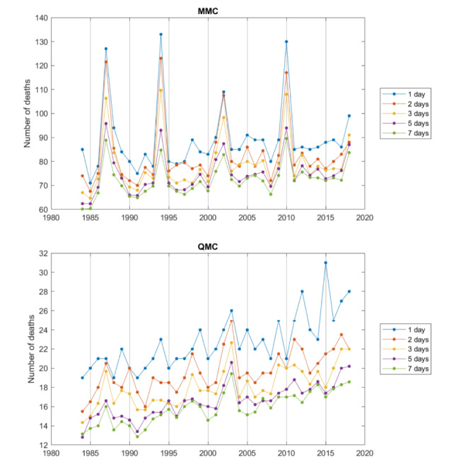
Number of deaths in each community for seleted durations. Graphs of the annual maximum of multi-day averages of daily mortality over selected durations during the summer season for each community
In the formulation of the MDF relationship, the return level of  for a given return period of
  years is given by:
 |
1 |
An advantage of this formulation is that  has a separable functional dependence on
  and
and  .
.  is a function that defines parallel curves for the different return periods.
  is a function that modulates the shape of the MDF curves as a function of the duration and is defined in this study by:
 |
2 |
where η is a shape parameter subject to the constraint that  . If
. If  have a certain distribution
  , then
  will also have the same distribution and consequently
  . The generalized extreme value (GEV) probability distribution is proposed here to model
  . The use of the GEV is justified by the fact that it is theoretically the limiting distribution for block maxima (Coles 2001). The quantile function of GEV is given by:
 |
3 |
where μ, σ and κ are the location, scale and shape parameters respectively. Parameters are subject to the constraints that  and σ . The general MDF relationship is then given by the following expression:
 |
4 |
In the non-stationary framework, the distribution parameters are made dependent on covariates representing any processes that drive the response variable. Note that non-stationarity does not necessarily imply the existence of trend (or even change), and stationarity does not necessarily imply that the phenomena being modeled are static. Non-stationarity characterizes all natural phenomena. In this work, the use of the term non-stationary of a model refers simply to the fact that the parameters of the model are function of covariates that represent the processes that control the output variable being modeled.
Let us denote  and
and  , two time-dependent covariates. For nonstationary models with one covariate, the location parameter can be stationary or can depend linearly or quadratically on
  :
:
 |
5 |
and the log-transformed scale parameter can be stationary or can depend linearly on  :
:
 |
6 |
For nonstationary models with two covariates, the location parameter can be stationary or can depend linearly or quadratically on  and
and  :
:
 |
7 |
and the log-transformed scale parameter can be stationary or can depend linearly on  and
and  :
:
 |
8 |
The shape parameters κ, and  , are kept constant, which is an assumption commonly made in nonstationary models (Katz et al. 2002; El Adlouni et al. 2007; Ouarda and Charron 2019). The relationships of the distribution parameter
  with the covariates are restricted to the linear form. These latter limitations were imposed for reasons of parsimony because the number of model parameters increases rapidly with the complexity of the model and the record size can become a limiting factor. The nonstationary models are built by considering any combinations of functional dependency in Eqs. (5) and (6) for one covariate and in Eqs. (7) and (8) for two covariates. The case where both distribution parameters are constant (
 and
and  ) is equivalent to the stationary model.
The two covariates introduced here are a climate index and time, representing the temporal trend. The climate index covariate is defined by the lagged 3-month average of a climate index with the most significant impacts on the response variable. The covariate of the temporal trend is defined by a series of integers incremented from 1 to the number of years required by the application. When n is larger than the number of years of observations, MDF relationships are extrapolated.
Maximum composite likelihood method
The method used here for the estimation of the distribution parameter vector  is the maximum composite likelihood (Varin et al. 2011). This method is adopted instead of the classical maximum likelihood approach because of the particular formulation of the nonstationary MDF model. Indeed, while observations from year to year can be considered as independent, the observations over the different durations for the same year are often dependent. Let us define
  , the joint probability density of the random vector
  where α is a parameter vector that parameterizes the interdependence between the values corresponding to different durations and
  , defined above, parameterizes the marginal structure (Chandler and Bate 2007). The likelihood function that considers these factors, called full likelihood, is then given by:
 |
9 |
where  denotes the maximum average mortality for the year
  and for the duration group
  . A major difficulty of this approach is that
  is usually unknown. To overcome this problem, a simplified likelihood function, called independence likelihood (Chandler and Bate 2007), can be obtained by assuming the observations over the different durations to be independent (Muller et al. 2008; Van de Vyver 2015). This simplified function is derived by multiplying a set of component likelihoods (Varin et al. 2011) and can be considered as the simplest case of a composite likelihood. Given that
  represents the density function of
  , the independence likelihood is given by:
 |
10 |
Composite likelihood is often used in applications as surrogate for the full likelihood when it is too cumbersome or impossible to compute (Varin and Vidoni 2005). By assuming that  follows a GEV distribution, the probability function of
  is given by (Muller et al. 2008):
 |
11 |
In the nonstationary case, the distribution parameters  and
and  become time-dependent and are expressed by:
 |
12 |
To find  , the estimate of
  that maximizes
  , an optimization procedure should be used. In practice, the log likelihood
  is maximized instead of
  . In this study, the optimization function fmincon in Matlab® is used to find
  .
.
For model comparison, the Akaike information criterion (AIC) or the Bayesian information criterion (BIC) are frequently used in statistics. They are defined by:
 |
13 |
 |
14 |
where q is the number of parameters in the model. Such criteria account for the goodness-of-fit and penalize models with more parameters. Because of the assumption of independence among the likelihood terms in the definition of the independence likelihood, composite likelihood can be seen as a misspecified likelihood and the classical definitions should be generalized (Varin et al. 2011). Analogous criteria for AIC and BIC based on composite likelihoods were introduced (Varin and Vidoni 2005) and have the following forms (Varin et al. 2011):
 |
15 |
 |
16 |
where  is the effective number of parameters estimated by
  ,
,  is the sensitivity or Hessian matrix and
  is the variability matrix. The sample estimates of
  and
and  can be obtained by:
 |
17 |
 |
18 |
where  and
and  denotes the vector of maximum average number of deaths for the year
  . Given that the second Bartlett identity is valid for each individual likelihood term, the cumbersome computation of the matrix
  can be obtained alternatively by (Varin et al. 2011):
 |
19 |
Data
The data used in the present study consist in the overall all-cause daily mortality within each community from 1983 to 2018 and are provided by the National institute of public health of Quebec (INSPQ). Gridded estimates of mean daily temperatures (average of the minimum and maximum temperatures) from the Daymet (Thornton et al. 2020) data product were spatially averaged over the area covered by each community during the same period. From the raw temperature time series, heat wave events were extracted. Although there is no standard definition of heat waves, a basic definition of a heat wave generally implies an extended period of unusually high atmosphere-related heat stress (Robinson 2001). For illustration purposes, heat wave events are defined here as periods of at least two days with a mean daily temperature above the 90th percentile of historical summer (June-August) (Oudin Åström et al. 2013) temperature in a given region. Figure 2 illustrates the impact of the heat wave events on the mortality in 2010 in the MMC. The first heat event had a significant impact on mortality as the daily mean temperature reached near 29 °C and the wave extended over several days. The other two heat events were shorter and less severe, and thus had no significant impact on daily mortality.
Fig. 2.
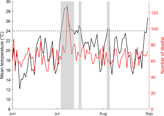
Impact of heat wave events on the daily number of deaths. The mean daily temperature is plotted with the daily number of deaths for the MMC during the summer of 2010. Heat wave events are identified by shaded areas
Climate index time series are available from the NOAA Physical Sciences Laboratory database (https://psl.noaa.gov/data/climateindices/list/). The Atlantic multi-decadal oscillation (Trenberth and Shea 2006) index is obtained by applying a low-pass filter on area average sea surface temperature (SST) anomalies in the North Atlantic basin between 0 and 60°N. The AO is identified through an empirical orthogonal function (EOF) analysis of monthly mean 1000-hPa height anomalies over the northern extratropics. The NAO is the surface sea-level pressure difference between the Subtropical (Azores) High and the Subpolar Low. The NAO pattern is obtained from the first mode of a Rotated Empirical Orthogonal Function (REOF) analysis using standardized monthly 500 millibar height anomaly data between January 1950 and December 2000 over latitude 20–90°N. The second mode of the REOF yields the PNA pattern. The Pacific Decadal Oscillation (PDO) index is the leading principal component from an un-rotated Empirical Orthogonal Function (EOF) analysis of monthly SST anomalies in the North Pacific Ocean, typically, polewards of 20°N (Mantua and Hare 2002). The Southern Oscillation index (SOI) compares the standardized monthly sea level pressure anomalies between Tahiti and Darwin, Australia.
Results
The proposed non-stationary MDF approach is applied to observed daily mortality in the Montreal Metropolitan Community (MMC) and the Quebec Metropolitan Community (QMC). All-cause mortality is chosen consistently with the current state-of-the-art literature (Masselot et al. 2023; Martinez-Solanas et al. 2021; Gasparrini et al. 2015), given that the mortality risk of extreme heat is consistent across a wide range of diseases (Burkart et al. 2021). With a population of around 4 Million and 0.8 Million respectively, they are the two most populated agglomerations east of Toronto in Canada. These communities recently experienced severe heat waves, especially Montreal. Note that MMC is on average 3 °C warmer than QMC. The heat wave during July 2010 caused a significant increase of 33% in the crude death rate in the province (Bustinza et al. 2013).
To build the MDF curves, the annual maximum of multi-day averages of daily mortality over durations of 1 to 7 days during the summer season were extracted for each community. A positive trend in the annual maximum mortality time series was observed in all durations for both agglomerations. The potential impacts of large-scale modes of variability on daily mortality are explored here. For this, for each selected climate index, seasonal values were calculated (seasonal indices) using a moving window of 3-month average (Ouarda et al. 2019a, b) values to identify the seasons with the greatest impact on maximum mortality during the summer season. The correlations between the seasonal indices of the different lags and the detrended maximum mortality time series for the different durations were calculated for each community. The seasonal climate indices leading to the maximum significant correlations for the different durations represent good predictors of the mortality and are hence selected as candidate covariates. In general, we consider three-month windows that took place before the summer for which the mortality extremes are being analyzed. This is important as we are looking for covariates to serve as predictors of the mortality extremes and hence, they need to be available before the summer season of these extremes.
Table 1 illustrates the correlations obtained for the MMC with the selected climate indices for the optimal selected seasons. Results for the MMC are illustrated because the impacts are easier to detect than for QMC due to its larger population. The Student’s t-test is used to determine the significance of the correlations at a level of 10%. The AMO index, known to have a significant influence on extreme summer temperatures in North America (Sutton and Hodson 2005) has a relatively weak impact here. AMO is a low frequency multi-decadal mode of variability and the length of one cycle may be too large for the relatively short observational period in this study to see a clear signal. Table 1 indicates that the North Atlantic Oscillation (NAO) index averaged for the 3-month season of July-August-September (JAS) during the preceding year (denoted NAO(JAS−1) has the most important correlations for the MMC. Table 1 indicates that the SOI, PDO and PNA have correlations with mortality higher than 20% for all durations. Correlations are significant for SOI and for 1-day to 3-day durations and are also significant for PDO and PNA for the 1-day duration. It is important to highlight that all indices selected for the model must be defined for months that occur either in the preceding year, or in the current year but before the summer season. This is important as these indices will serve as predictors for the summer extreme mortality events. It is also relevant to note that no causality tests were carried out in the present study. The approach we adopted tries effectively to explain a larger part of the data variability through the use of the climate oscillation covariates.
Table 1.
Correlation coefficients between the annual maximum of the mean mortality (detrended time series) and seasonal climate indices used as covariates in the nonstationary MDF relationship for the MMC area
| Climate index | Season | Duration | ||||||
|---|---|---|---|---|---|---|---|---|
| 1-day | 2-day | 3-day | 4-day | 5-day | 6-day | 7-day | ||
| AMO | MAM | 0.18 | 0.16 | 0.12 | 0.11 | 0.12 | 0.15 | 0.15 |
| NAO | JAS−1 | -0.38** | -0.41** | -0.41** | -0.43** | -0.45** | -0.43** | -0.41** |
| SOI | MAM | -0.30* | -0.34** | -0.29* | -0.27 | -0.24 | -0.22 | -0.23 |
| PDO | NDJ | 0.30* | 0.26 | 0.23 | 0.25 | 0.23 | 0.20 | 0.20 |
| PNA | OND−1 | 0.28* | 0.23 | 0.22 | 0.24 | 0.26 | 0.24 | 0.23 |
−1 denotes a season occurring before the current year
* denotes correlations statistically significant at p < .10.
** denotes correlations statistically significant at p < .05.
Bold indicates significant correlations at all levels considered
For illustration purposes, the impacts of the seasonal NAO index and long-term trend on heat waves are presented here. A conditional Poisson-Generalized Pareto model (Katz et al. 2002; Ouarda et al. (2019a, b) was fitted to the heat wave frequency and intensity time series in the MMC. The covariate NAO (JAS−1) that has been identified as most correlated with mortality and the temporal trend (year) were used as covariates. Figure 3 presents the frequency of heat events in the MMC as a function of the Time and NAO(JAS−1) covariates. The graphs show the combined effect of the NAO index and the long-term trend. The negative relationship between NAO and the heat wave frequency and intensity can be noticed. An increasing temporal trend in the frequency and intensity of heat waves, independently of the effect of NAO, can also be noticed.
Fig. 3.

Frequency and intensity of heat waves in the MMC as a function of the NAO index and the time. (a) Median quantile of the frequency of heat waves modeled with the Poisson distribution as a function of the covariate NAO (JAS-1) and Time. (b) Median quantile of the intensity of heat waves modeled with the generalized Pareto distribution as a function of the covariate NAO(JAS−1) and Time (b)
The nonstationary MDF model was fitted to the mortality data in both communities (see details of the model in the Method section). The covariate representing the temporal trend is denoted here “Time”. One nonstationary model uses only Time as covariate (denoted MDF model “Time”). A second one uses a single climate index (denoted MDF model “NAO”, for instance) and a third model uses Time combined with a climate index (denoted MDF model “Time + NAO”, for instance). The criterion CL-AIC (see Eq. (15)), an analogue of the Akaike information criterion (AIC) based on composite likelihood (CL), is used for model comparison. CL-AIC accounts for the goodness of-fit and penalizes the more complex models with more parameters. For each model with a climate index, the optimal seasonal index in Table 1 was used.
Table 2 presents the maximized independence log-likelihood (LL), the CL-AIC statistic and the model parameters for each MDF model obtained for both communities. The CL-AIC results in Table 2 represent a verification of the MDF relationships developed for the two metropolitan areas considered in this study. For a given selection of covariates, the relationships between model parameters and covariates are optimal relative to the CL-AIC. In all cases, with respect to the CL-AIC, nonstationary models lead to a substantial improvement in the goodness-of-fit in comparison to stationary models. This is so despite the penalty associated to nonstationary models in terms of CL-AIC because of their higher number of parameters. This indicates that nonstationary models provide a better fit to the data even when penalized for parsimony. The simple MDF Time model significantly improves the stationary model, and this improvement turns out to be superior to the one obtained with any model with only one teleconnection covariate. This underlines the importance of including climate change signal in modeling maximum summer mortality and indicates also that climate change signal is more important than climate variability signal in explaining maximum summer mortality for both the MMC and the QMC.
Table 2.
Stationary and nonstationary MDF relationships fitted to the data of the regions under study
| Region | Model | LL | CL-AIC | μ *t | σ *t | η |
|---|---|---|---|---|---|---|
| MMC | Stationary | -856.58 | 1748.53 | 82.83 | 2.09 | 0.098 |
| Time | -795.61 | 1632.72 |

|
1.66 | 0.088 | |
| AMO | -820.30 | 1682.22 |
|
1.83 | 0.098 | |
| Time + AMO | -793.64 | 1637.00 |
|
1.65 | 0.089 | |
| NAO | -790.66 | 1630.93 |
|
1.65 | 0.087 | |
| Time + NAO | -774.95 | 1618.92 |
|

|
0.091 | |
| SOI | -854.62 | 1757.78 | 82.66 |

|
0.096 | |
| Time + SOI | -791.57 | 1631.93 |

|
1.62 | 0.088 | |
| PDO | -835.94 | 1739.65 |

|

|
0.088 | |
| Time + PDO | -795.28 | 1639.79 |

|
1.66 | 0.088 | |
| PNA | -846.23 | 1737.61 |
|
2.05 | 0.100 | |
| Time + PNA | -777.38 | 1619.68 |

|

|
0.085 | |
| QMC | Stationary | -507.38 | 1042.77 | 21.48 | 0.72 | 0.187 |
| Time | -393.82 | 818.41 |

|
0.06 | 0.172 | |
| AMO | -468.72 | 968.91 |

|
0.46 | 0.175 | |
| Time + AMO | -393.81 | 822.91 |

|
0.06 | 0.172 | |
| NAO | -468.87 | 975.28 |

|
0.44 | 0.182 | |
| Time + NAO | -381.52 | 797.80 |

|
-0.04 | 0.170 | |
| SOI | -507.30 | 1052.29 | 21.49 |

|
0.187 | |
| Time + SOI | -380.97 | 816.80 |
|

|
0.178 | |
| PDO | -502.14 | 1038.97 | 21.54 |

|
0.189 | |
| Time + PDO | -379.98 | 803.96 |

|

|
0.179 | |
| PNA | -500.77 | 1042.44 |
|
0.70 | 0.188 | |
| Time + PNA | -379.08 | 804.09 |

|

|
0.180 |
* The relationships of the model parameters with the covariates are the optimal configurations with respect to CL-AIC
The models combining a climate index with Time lead generally to a better performance than the MDF Time model (or any model with a single teleconnection covariate), despite the parsimony penalty. This means that climate indices successfully explain a part of the interannual variability in the maximum summer mortality. Overall, the best results are obtained with the MDF Time + NAO model for both communities, consistently with the correlations of Table 1. PNA is also a good candidate according to the LL and CL-AIC scores.
Stationary MDF curves would be represented on graphs with the intensity plotted against the duration where each curve represents a return period. In the nonstationary framework, curves cannot represent the complete model because of the increase in dimensionality. However, response surfaces can be represented in a three-dimensional plot after reduction of the graph’s dimensionality by setting the duration, the return period or some of the covariates to fixed values. Examples of such graphs are presented in Fig. 4 with the MDF Time + NAO model for the MMC and QMC. MDF surfaces are shown for different return periods where the duration is fixed to two days (Fig. 4ab) and for different durations where the return period is fixed to 5 years (Fig. 4cd). Figure 4 also provides predictions of intensity, duration and return periods until 2034 to show the expected evolution in the coming decade. In Fig. 4, the covariate Time was extended to the year 2034 to illustrate the predictive mode of the model. Such a tool provides predictions of the expected maxima of mortality due to climate, that is characterized jointly by the magnitude and duration, and thus of expected stress on the health system.
Fig. 4.

Nonstationary MDF surfaces for the MMC and the QMC extended until 2034. Nonstationary MDF surfaces are shown for the MMC (a, c) and the QMC (b, d) as a function of the covariates Time and NAO. The summer mortality is presented for different return periods and a duration of 2 days (a, b) and for different durations and a return period of 5 years (c, d)
MDF surfaces can also be obtained for a specific year of interest. Such graphs are illustrated in Fig. 5, where Time is set to 2030. The figure presents the predictions of the nonstationary MDF surfaces of the modelled number of deaths for the MMC and QMC for the year 2030, as a function of the NAO values and the duration of the event (from 1 to 7 days). Parallel surfaces show the various frequencies of interest. As the horizon of 2030 approaches, predictions of the value of the NAO become available and that restricts the range of the response surfaces. On October 2029, the value of the predictor NAO(JAS−1) (mean NAO value for the months of July-August-September of the year before the prediction year) is known and it is possible to have a much more precise prediction based on the state of the NAO index. Needless to say, a more precise prediction would be obtained if we also integrate the information concerning other climate oscillation indices of interest for the MMC and QMC. The development of MDF models that are conditioned on more than one climate oscillation index will make these models more reliable and more useful in practice.
Fig. 5.

Projections of nonstationary MDF surfaces (summer mortality) for the MMC and the QMC for the year 2030. The nonstationary MDF surfaces for the MMC (a) and the QMC (b) with the covariate Time and NAO(JAS−1) where the time is set at the year 2030
A question can be raised concerning the contribution of population growth and population aging to extreme daily mortality and to the observed temporal trend. Figure 6 presents graphs of the Standardized (per 100000 persons) annual maximum of multi-day averages of daily mortality over selected durations during the summer season for each community. These graphs indicate that standardization by the population size leads to a smaller positive temporal trend for the QMC, and a reversal of trend for the MMC. The number of standardized daily deaths decreases in MMC which indicates that the impact of climate warming is compensated for by human adaptation to heat, the adaptation measures adopted in the city of Montreal (measures to reduce heat island effect, green roofing, air-conditioning availability, etc.) and the fact that the population of the city of Montreal is younger than the population of the city of Quebec (a more administrative city). In the QMC, even when the effect of population increase is eliminated, the standardized number of daily deaths maintains a positive trend, reflecting among others the impact of climate change.
Fig. 6.
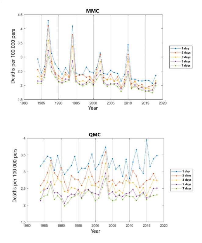
Standardized (per 100000 persons) number of daily deaths in each community for seleted durations. Graphs of the standardized annual maximum of multi-day averages of daily mortality over selected durations during the summer season for each community
Discussion
The proposed nonstationary approach leads to MDF relationships that are conditional on time-dependent covariates. The covariates used here are the long-term trend (representing climate change) and climate oscillation patterns (representing climate variability). The use of climate oscillation patterns is justified by the fact that they are good predictors of heat waves (Loikith and Broccoli 2014; Chandran et al. 2016), which in turn influence the daily mortality. The fact the temporal trend persists in the model despite the inclusion of climate indices suggests that it captures additional source of change in mortality, such as demographic and climate changes.
The results obtained herein show that the goodness-of-fit is improved with the use of the nonstationary approach with covariates. The impacts of taking into account the time trend are crucial because of the large trend component of the mortality time series. The temporal trend covariate accounts for climate change but also for other sources of trends not related to climate such as population changes, aging, air conditioning availability, etc. When climate indices are introduced in addition to the temporal trend covariate, the goodness-of-fit is improved in comparison to the model introducing the temporal trend only despite the parsimony penalty resulting from the larger number of parameters in the model. Indeed, the use of dedicated estimation and model selection procedure, in particular the CL-AIC, reduces the risk of overfitting given its penalized nature and associated properties. In various contexts, the AIC has been shown to be equivalent to a leave-one-out cross-validation (Fang 2022).
This means that climate indices successfully explain a part of the interannual variability in the maximum summer mortality. This is an original result that underlines the importance of integrating climate change in mortality predictions, but also the importance of including climate variability indices in public health planning models. To the knowledge of the authors, no country has integrated teleconnection information in their heat-health watch and warning systems or their heat-health adaptation plans.
Figure 3 indicates a linear response of mortality as a function of NAO values for QMC, while the relationship seems to be non-linear for MMC. The two communities are relatively close (less than 300 km) and hence, the response to the various low frequency climate oscillation indices should be relatively similar. The difference in response should be due to other variables, such as average age (MMC population is younger) or mean summer temperatures (QMC is on average 2 °C colder than Montreal during summer). Models integrating additional covariates should provide more detailed information about specific communities and would be of special interest for public health managers at the regional and local scales.
Figure 6 illustrates the importance of having the temporal component in the nonstationary model. This component takes into consideration a number of important factors such as climate change, population adaptation, population aging, municipal measures to reduce heat island effect, etc. The presence of the temporal trend component does not disturb the signal of the climate oscillation index, and the two signals provide complementary information.
Aside from NAO, it is important to mention that other indices enter into play and their effect is not linear with the NAO. This is so because these indices do not have the same cycle length, so their effects sometimes cumulate and sometimes cancel each other. The CMM and CMQ are in a region strongly influenced by the Atlantic modulations but also the Arctic and the Pacific, and as so this represents a region where teleconnection analysis is among the most complex. For instance, AMO has positive and negative phases that are on the average around 30 years long, while ENSO periods range between 3 and 7 years, and AO oscillations occur around every two years. Even the tropical Atlantic Ocean itself exhibits two primary modes of interannual variability: the “equatorial mode” analogous to the Pacific El Nino phenomenon (ENSO) and a “dipole” mode without a Pacific counterpart. The integration of NAO in the model helps explain an additional part of the interannual variability but does not explain all modulations. Future work should focus on building models that integrate more than one index as covariate. The model presented in the present paper is a first step towards the development of public health models that take into consideration teleconnection effects. As more data becomes available, it will be possible to build models with more covariates.The proposed model allows also introducing other covariates than climatic ones. For instance, the population density and average age, and the deprivation index are potential candidates for covariates that could improve the model. Mean summer temperature can also be introduced as covariate even if a part of the signal is already included in the climate indices.
The nonstationary MDF relationships are useful in public health management and allow integrating information concerning future climatic and socio-economic or demographic scenarios into the model, while providing projections about the magnitude and duration of future heat wave mortality. Seasonal predictions of the occurrence of waves of mortality can be obtained directly as the climatic indices used in the model are readily available from observations before the summer heat episodes, therefore helping public health officials in the preparation of the next summer months in advance.
The approach presented herein still has a number of limitations. First, as the MDF focuses on the maximum of each year, it does not necessarily represent well the whole annual heat-related mortality. In addition, in summers that are not exceptionally hot, the maximum intensity of the number of deaths can probably be unrelated to excess heat. Finally, the all-cause mortality approach used here includes several causes unrelated to heat waves and can therefore blur the signal by mixing excess heat deaths with deaths from other causes. Still, the model leads to good results and provides useful information that goes beyond the information provided by other health planning and heat-health warning models, such as the worst-case scenario that can be expected by health services planners.
Future efforts should focus on overcoming the limitations listed above by considering over-mortality values, eliminating infectious-disease events, such as salmonella outbreaks or COVID-19, integrating additional climatic and non-climatic covariates (such as population density, population growth, average population age, deprivation index, average family size, mean summer temperatures, atmospheric pollution levels, presence and magnitude of heat island effect, etc.), developing regional models that take into consideration the specificities of each region, and adopting an all-peaks-over-threshold approach (Ribatet et al. 2009). The model should also be applied to different regions of the world under different climatic drivers. As the observational period becomes longer, the record lengths will encompass several cycles of the low frequency multi-decadal modes of variability (such as AMO) and the performance of the models will further improve. Once models that take into consideration the regional specificities are built, it will be possible to develop regional models that estimate the MDF relationships at ungauged locations based on the covariates used to describe each region, in a similar way ungauged basin models are built in hydrological frequency analysis (see for instance Cavadias et al. 2001; Seidou et al. 2006; and Castellarin et al. 2013).
Funding for this research was partially provided by the AUDACE program of the Fonds de Recherche du Québec (FRQ). The authors are also thankful to the Natural Sciences and Engineering Research Council of Canada (NSERC) and the Canada Research Chairs Program for co-funding this research. The authors thank Mr. Christian Charron for his assistance. The authors wish to express their appreciation to Pr. Alin Andrei Carsteanu, Editor, Pr. César Aguilar and a second anonymous reviewer for their invaluable comments and suggestions which helped improve the quality of the paper.
Electronic supplementary material
Below is the link to the electronic supplementary material.
Acknowledgements
The authors thank Mr. Christian Charron for his assistance.
Author contributions
T.B.M.J.O: Conceptualization, Methodology, Software, Formal analysis, Investigation, Resources, Writing - Original Draft, Project administration, Funding acquisition. P.M.,C.E., P.G., E.L., A.S-H., F.C and P.V: Writing - Review & Editing, Validation.
Data availability
No datasets were generated or analysed during the current study.
Declarations
Competing interests
The authors declare no competing interests.
Footnotes
Publisher’s note
Springer Nature remains neutral with regard to jurisdictional claims in published maps and institutional affiliations.
References
- Anderson GB et al (2018) Projected trends in high-mortality heatwaves under different scenarios of climate, population, and adaptation in 82 US communities. Clim Change 146(3):455–470. 10.1007/s10584-016-1779-x [DOI] [PMC free article] [PubMed] [Google Scholar]
- Andersson-Sköld Y et al (2015) An integrated method for assessing climate-related risks and adaptation alternatives in urban areas. Clim Risk Manage 7:31–50. 10.1016/j.crm.2015.01.003 [Google Scholar]
- Basha G et al (2017) Historical and projected Surface temperature over India during the 20th and 21st century. Sci Rep 7(1):2987. 10.1038/s41598-017-02130-3 [DOI] [PMC free article] [PubMed] [Google Scholar]
- Bayentin L et al (2010) Spatial variability of climate effects on ischemic heart disease hospitalization rates for the period 1989–2006 in Quebec, Canada. Int J Health Geogr 9:5. 10.1186/1476-072X-9-5 [DOI] [PMC free article] [PubMed] [Google Scholar]
- Burkart KG et al (2021) (2021) Estimating the cause-specific relative risks of non-optimal temperature on daily mortality: a two-part modelling approach applied to the Global Burden of Disease Study. The Lancet 398(10301):685–697 [DOI] [PMC free article] [PubMed] [Google Scholar]
- Bustinza R et al (2013) Health impacts of the July 2010 heat wave in Québec, Canada. BMC Public Health 13(1):56. 10.1186/1471-2458-13-56 [DOI] [PMC free article] [PubMed] [Google Scholar]
- Casanueva A et al (2019) Overview of existing heat-health warning systems in Europe. Int J Environ Res Public Health. 10.3390/ijerph16152657 [DOI] [PMC free article] [PubMed] [Google Scholar]
- Castellarin A et al (2013) Prediction of flow duration curves in ungauged basins, in Runoff Prediction in Ungauged Basins: Synthesis across Processes, Places and Scales, edited by G. Bloschl., University Press, Cambridge, 135–162
- Cavadias G et al (2001) A canonical correlation approach to the determination of homogeneous regions for regional flood estimation of ungauged basins. Hydrol Sci J 46(4):499–512 [Google Scholar]
- Chandler RE, Bate S (2007) Inference for clustered data using the independence loglikelihood. Biometrika 94(1):167–183. 10.1093/biomet/asm015 [Google Scholar]
- Chandran A et al (2016) Influence of climate oscillations on temperature and precipitation over the United Arab Emirates. Int J Climatol 36(1):225–235. 10.1002/joc.4339 [Google Scholar]
- Cheng J et al (2019) Cardiorespiratory effects of heatwaves: a systematic review and meta-analysis of global epidemiological evidence. Environ Res 177:108610. 10.1016/j.envres.2019.108610 [DOI] [PubMed] [Google Scholar]
- Coles S (2001) An introduction to statistical modeling of extreme values. Springer, London [Google Scholar]
- Coumou D, Robinson A (2013) Historic and future increase in the global land area affected by monthly heat extremes. Environ Res Lett 8(3):034018. 10.1088/1748-9326/8/3/034018 [Google Scholar]
- El Adlouni S et al (2007) Generalized maximum likelihood estimators for the nonstationary generalized extreme value model. Water Resour Res 43(3):W03410. 10.1029/2005WR004545 [Google Scholar]
- Fang Y (2022) Asymptotic equivalence between cross-validations and Akaike Information Criteria in mixed-effects models. J Data Sci 9(1):15–21 [Google Scholar]
- Gasparrini A et al (2015) Mortality risk attributable to high and low ambient temperature: a multicountry observational study. Lancet 386(9991):369–375 [DOI] [PMC free article] [PubMed] [Google Scholar]
- Guo Y et al (2018) Quantifying excess deaths related to heatwaves under climate change scenarios: a multicountry time series modelling study. PLoS Med 15(7):e1002629. 10.1371/journal.pmed.1002629 [DOI] [PMC free article] [PubMed] [Google Scholar]
- Jacques-Coper M et al (2021) Intraseasonal teleconnections leading to heat waves in central Chile. Int J Climatol 41(9):4712–4731. 10.1002/joc.7096 [Google Scholar]
- Katz RW et al (2002) Statistics of extremes in hydrology. Adv Water Resour 25(8–12):1287–1304. 10.1016/S0309-1708(02)00056-8 [Google Scholar]
- Kingsborough A et al (2017) Development and appraisal of long-term adaptation pathways for managing heat-risk. Lond Clim Risk Manage 16:73–92. 10.1016/j.crm.2017.01.001 [Google Scholar]
- Koutsoyiannis D et al (1998) A mathematical framework for studying rainfall intensity-duration-frequency relationships. J Hydrol 206(1–2):118–135 [Google Scholar]
- Laz OU, Rahman A, Ouarda TBMJ, Jahan N (2023) Stationary and non-stationary temperature-duration-frequency curves for Australia. Stoch Env Res Risk Assess 37:4459–4477. 10.1007/s00477-023-02518-w [Google Scholar]
- Lee T, Ouarda TBMJ (2011) Prediction of climate nonstationary oscillation processes with empirical mode decomposition. J Geophys Research: Atmos 116(D6):D06107. 10.1029/2010jd015142 [Google Scholar]
- Loikith PC, Broccoli AJ (2014) The influence of recurrent modes of climate variability on the occurrence of winter and summer extreme temperatures over North America. J Clim 27(4):1600–1618. 10.1175/jcli-d-13-00068.1 [Google Scholar]
- Mantua NJ, Hare SR (2002) The pacific decadal oscillation. J Oceanogr 58(1):35–44 [Google Scholar]
- Martínez-Solanas È et al (2021) Projections of temperature-attributable mortality in Europe: a time series analysis of 147 contiguous regions in 16 countries. Lancet Planet Health 5(7):e446–e54 [DOI] [PubMed] [Google Scholar]
- Masselot P et al (2018) A new look at weather-related health impacts through functional regression. Sci Rep 8(1):15241. 10.1038/s41598-018-33626-1 [DOI] [PMC free article] [PubMed] [Google Scholar]
- Masselot P et al (2023) Excess mortality attributed to heat and cold: a health impact assessment study in 854 cities in Europe. Lancet Planet Health 7(4):e271–e281 [DOI] [PubMed] [Google Scholar]
- McCabe G et al (2004) J Pacific and Atlantic Ocean influences on multidecadal drought frequency in the United States. Proc Natl Acad Sci 101 12 4136–4141 10.1073/pnas.0306738101 [DOI] [PMC free article] [PubMed] [Google Scholar]
- Meehl GA, Tebaldi C (2004) More intense, more frequent, and longer lasting heat waves in the 21st Century. Science 305(5686):994–997. 10.1126/science.1098704 [DOI] [PubMed] [Google Scholar]
- Mo KC et al (2009) Influence of ENSO and the Atlantic multidecadal oscillation on drought over the United States. J Clim 22(22):5962–5982 [Google Scholar]
- Muller A et al (2008) Bayesian comparison of different rainfall depth–duration–frequency relationships. Stoch Env Res Risk Assess 22(1):33–46. 10.1007/s00477-006-0095-9 [Google Scholar]
- Ning L, Bradley RS (2016) NAO and PNA influences on winter temperature and precipitation over the eastern United States in CMIP5 GCMs. Clim Dyn 46(3):1257–1276. 10.1007/s00382-015-2643-9 [Google Scholar]
- Odame EA et al (2018) Assessing Heat-Related Mortality Risks among Rural Populations: A Systematic Review and Meta-Analysis of Epidemiological Evidence. Int J Environ Res Public Health. 10.3390/ijerph15081597 [DOI] [PMC free article] [PubMed] [Google Scholar]
- Ouarda TBMJ, Charron C (2018) Nonstationary temperature-duration-frequency curves. Sci Rep 8(1):15493. 10.1038/s41598-018-33974-y [DOI] [PMC free article] [PubMed] [Google Scholar]
- Ouarda TBMJ, Charron C (2019) Changes in the distribution of hydro-climatic extremes in a non-stationary framework. Sci Rep 9(1):8104. 10.1038/s41598-019-44603-7 [DOI] [PMC free article] [PubMed] [Google Scholar]
- Ouarda TBMJ et al (2019a) Nonstationary warm spell frequency analysis integrating climate variability and change with application to the Middle. East Clim Dynamics 53(9–10):5329–5347. 10.1007/s00382-019-04866-2 [Google Scholar]
- Ouarda TBMJ et al (2019b) Non-stationary intensity-duration-frequency curves integrating information concerning teleconnections and climate change. Int J Climatol 39(4):2306–2323. 10.1002/joc.5953 [Google Scholar]
- Oudin Åström D et al (2013) Attributing mortality from extreme temperatures to climate change in Stockholm. Swed Nat Clim Change 3(12):1050–1054. 10.1038/nclimate2022 [Google Scholar]
- Pachauri RK et al (2014) Climate change 2014: synthesis report. Contribution of Working Groups I, II and III to the fifth assessment report of the Intergovernmental Panel on Climate Change, IPCC
- Perkins-Kirkpatrick SE, Lewis SC (2020) Increasing trends in regional heatwaves. Nat Commun 11(1):3357. 10.1038/s41467-020-16970-7 [DOI] [PMC free article] [PubMed] [Google Scholar]
- Ribatet M et al (2009) Modeling all exceedances above a threshold using an extremal dependence structure: inferences on several flood characteristics. Water Resour Res 45(3):W03407. 10.1029/2007wr006322 [Google Scholar]
- Robinson PJ (2001) On the definition of a Heat Wave. J Appl Meteorol 40(4):762–775. https://doi.org/10.1175/1520-0450(2001)040<0762:otdoah>2.0.co;2 [Google Scholar]
- Russo S et al (2014) Magnitude of extreme heat waves in present climate and their projection in a warming world. J Geophys Research: Atmos. 10.1002/2014JD022098 [Google Scholar]
- Seager R et al (2005) Mechanisms of ENSO-forcing of hemispherically symmetric precipitation variability. Q J R Meteorol Soc 131(608):1501–1527. 10.1256/qj.04.96 [Google Scholar]
- Seidou O et al (2006) « a parametric bayesian combination of local and regional information in flood frequency analysis. Water Resour Res 42:W11408. 10.1029/2005WR004397 [Google Scholar]
- Sutton RT, Hodson DLR (2005) Atlantic Ocean Forcing of North American and European Summer Climate. Science 309(5731):115. 10.1126/science.1109496 [DOI] [PubMed] [Google Scholar]
- Thornton MM et al (2020) Daymet: Daily Surface Weather Data on a 1-km Grid for North America, Version 4. ORNL Distributed Active Archive Center
- Trenberth KE, Shea DJ (2006) Atlantic hurricanes and natural variability in 2005. Geophysical Research Letters 2006; 33(12)
- Van de Vyver H (2015) Bayesian estimation of rainfall intensity–duration–frequency relationships. J Hydrol 529:1451–1463. 10.1016/j.jhydrol.2015.08.036 [Google Scholar]
- Varin C, Vidoni P (2005) A note on composite likelihood inference and model selection. Biometrika 92(3):519–528. 10.1093/biomet/92.3.519 [Google Scholar]
- Varin C et al (2011) An overview of composite likelihood methods. Statistica Sinica 21(1):5–42 [Google Scholar]
- Vaughan C et al (2017) Creating an enabling environment for investment in climate services: the case of Uruguay’s National. Agricultural Inform Syst Clim Serv 8:62–71. 10.1016/j.cliser.2017.11.001 [Google Scholar]
- Vicedo-Cabrera AM et al (2021) The burden of heat-related mortality attributable to recent human-induced climate change. Nat Clim Chang 11(6):492–500. 10.1038/s41558-021-01058-x [DOI] [PMC free article] [PubMed] [Google Scholar]
- Wettstein JJ, Mearns LO (2002) The influence of the North Atlantic–Arctic Oscillation on Mean, Variance, and extremes of temperature in the Northeastern United States and Canada. J Clim 15(24):3586–3600, https://doi.org/10.1175/1520-0442(2002)015<3586:TIOTNA>2.0.CO;2.
- White CJ et al (2014) ENSO, the IOD and the intraseasonal prediction of heat extremes across Australia using POAMA-2. Clim Dyn 43(7):1791–1810. 10.1007/s00382-013-2007-2 [Google Scholar]
Associated Data
This section collects any data citations, data availability statements, or supplementary materials included in this article.
Supplementary Materials
Data Availability Statement
No datasets were generated or analysed during the current study.