Entropic Graph-based Posterior Regularization

Abstract

Graph smoothness objectives have achieved great success in semi-supervised learning but have not yet been applied extensively to unsupervised generative models. We define a new class of entropic graph-based posterior regularizers that augment a probabilistic model by encouraging pairs of nearby variables in a regularization graph to have similar posterior distributions. We present a three-way alternating optimization algorithm with closed-form updates for performing inference on this joint model and learning its parameters. This method admits updates linear in the degree of the regularization graph, exhibits monotone convergence, and is easily parallelizable. We are motivated by applications in computational biology in which temporal models such as hidden Markov models are used to learn a human-interpretable representation of genomic data. On a synthetic problem, we show that our method outperforms existing methods for graph-based regularization and a comparable strategy for incorporating long-range interactions using existing methods for approximate inference. Using genome-scale functional genomics data, we integrate genome 3D interaction data into existing models for genome annotation and demonstrate significant improvements in predicting genomic activity.¹

Graph-based methods have recently been successful in solving many types of semi-supervised learning problems (Chapelle et al., 2006; Das & Smith, 2011; Joachims, 1999; Subramanya et al., 2010; Subramanya & Bilmes, 2011; Zhu et al., 2004; Zhu & Ghahramani, 2002). These methods assume that data instances lie in a low-dimensional manifold that may be represented as a graph. They optimize a graph smoothness criterion, which states that data instances nearby in the graph should be more likely to receive the same label. In a semi-supervised learning setting, optimizing this criterion has the effect of spreading labels from labeled to unlabeled instances.

Despite the success of graph-based methods for semi-supervised learning, there has not been as much study of the use of graph smoothness objectives in an unsupervised setting. In unsupervised problems, we do not have labels but instead have a generative model that is assumed to explain the observed data given the latent labels. While some types of relationships between instances (for example, the relationship between neighboring words in a sentence or neighboring bases in a genome) can easily be incorporated into the generative model, it is often inappropriate to encode a graph smoothness assumption into the model this way, for two reasons. First, in some cases, it is not clear what probabilistic process generated the labels with respect to the graph. Some objectives and distance measures that are successful for semi-supervised learning do not have probabilistic analogues. Second, large models must obey factorization properties (e.g., a tree or chain as in hidden Markov models) to facilitate the use of efficient dynamic programming algorithms such as belief propagation. Graphs representing similarity between variables do not in general satisfy these structure requirements because they tend to be densely clustered, leading to very high-order factors.

In this paper, therefore, we propose a new regularization approach for expressing a graph smoothness objective over a probabilistic model. We employ the posterior regularization (PR) framework of Ganchev et al. (2010), in which a probabilistic model is regularized through a term defined on an auxiliary posterior distribution variable. We define a powerful posterior regularizer which encourages pairs of variables to have similar posterior distributions by adding a penalty based on their Kullback-Leibler (KL) divergence. The pairs of penalized variables are encoded in a regularization graph which may be entirely different from the graphical model on which inference is performed. This regularizer graph need not have low treewidth and admits efficient optimization even when fully connected. We call our strategy of adding KL regularization penalties entropic graph-based posterior regularization (EGPR).

We show that inference and learning using this regularizer can be performed efficiently using a three-way alternating optimization algorithm with closed-form updates. This algorithm alternates between (1) smoothing marginal posteriors according to a regularization similarity graph, (2) performing probabilistic inference in a graphical model with the same dependence structure as the unregularized model, and (3) updating model parameters. The updates are linear in the degree of the regularization graph and are easily parallelizable, in our experiments scaling to tens of millions of variables. We show that this procedure corresponds to a generalization of the EM algorithm.

We apply this approach to improve existing methods for annotating the human genome (Day et al., 2007; Hoffman et al., 2012a; Ernst & Kellis, 2010). Methods for genome annotation distill genomic data into a human-interpretable form by simultaneously partitioning the genome into non-overlapping segments and assigning labels to each segment. This type of analysis has recently had great success in interpreting the function of the human genome and formed an integral part of the analysis of the NIH-sponsored ENCODE project ((ENCODE Project Consortium, 2012; Hoffman et al., 2012b), http://www.nature.com/encode).

However, exiting annotation methods use temporal models such as hidden Markov models and therefore cannot efficiently incorporate data on the genome’s 3D structure. This 3D structure has been shown to play a key role in gene regulation and other genomic processes. In our experiments on synthetic data, a model using EGPR outperforms comparable models using either other regularization strategies (e.g., squared error) or loopy belief propagation. On ENCODE data, a model using EGPR predicts genome activity much more accurately than the currently-used chain models as well as other forms of regularizer. Thus EGPR provides a method for jointly modeling genome activity and 3D structure.

1. Proposed Method

In an unsupervised learning problem, we are given a set of vertices $V$ that index a set of $n=\left|V\right|$ random variables $X_V=\left\{X_1,\dots ,X_n\right\}$ and a conditional dependence graph $G=(V,E)$. The graphical model describes a probability distribution parameterized by $\theta$ that can be factorized as $p_{\theta }\left(x_V\right)=\frac{1}{Z}{\prod }_{C\in 𝒞}{\varphi }_{\theta }^{\left(C\right)}\left(x_C\right)$ where each $C\subseteq V$ is a fully connected clique in $G$. We denote random variables with capital letters (e.g., $X_H$) and instantiations of variables with lower-case (e.g., $x_H\in \text{domain}\left(X_H\right)$). We also use capitals to denote sets and lowercase to denote set elements (e.g., $X_h$ for $h\in H$). Training graphical models involves a set of observed data ${\bar{x}}_O$, where a subset of variables $O\subseteq V$ is observed and the remainder $H=V\setminus O$ are hidden.

When the probability distribution is governed by a set of parameters $\theta$, penalized maximum likelihood training corresponds to the optimization

$${\text{maximize}}_{\theta }J\left(\theta \right)\triangleq ℒ\left(\theta \right)+ℛ\left(\theta \right)$$ (1)

$$\text{where}ℒ\left(\theta \right)\triangleq \text{log}{p}_{\theta }\left({\bar{x}}_O\right)=\text{log}\sum _{x_H}{p}_{\theta }\left(x_H,{\bar{x}}_O\right),$$ (2)

and where $ℛ\left(\theta \right)$ is a regularizer that expresses prior knowledge about the parameters. Many regularizers are used in practice, such as the ${\ell }_2$ or ${\ell }_1$ norms, which encourage parameters to be small or sparse, respectively.

Instead of placing a regularizer on the parameters themselves, it is often more natural to place a regularizer on the posterior distribution, a technique called posterior regularization (Ganchev et al., 2010). This is done by introducing an auxiliary joint distribution $q\left(X_H\right)$, placing a regularizer on $q\left(X_H\right)$, and encouraging $q$ to be similar to $p_{\theta }$ via a KL divergence penalty. The regularizer is

$${ℛ}_{\text{PR}}\left(\theta \right)\triangleq \underset{q}{\text{max}}{ℛ}_{\text{PR}}^{\prime }(\theta ,q)$$ (3)

$${ℛ}_{\text{PR}}^{\prime }\left(\theta ,q\right)\triangleq -D\left(q\left(X_H\right)\Vert p_{\theta }\left(X_H\mid {\bar{x}}_O\right)\right)+𝒫ℛ\left(q\right),$$ (4)

where $D(\cdot \Vert \cdot )$ is the KL divergence $D\left(p\right(X)\Vert q(X\left)\right)={\sum }_{x}p\left(x\right)\text{log}\left(p\right(x)/q(x\left)\right)$ and $𝒫ℛ\left(q\right)$ is a penalty term that expresses some prior knowledge about the posterior distribution. For notational convenience, we also define $J^{\prime }(\theta ,q)\triangleq ℒ\left(\theta \right)+{ℛ}^{\prime }(\theta ,q)$. Ganchev et al. (2010) showed how to optimize this combined objective efficiently when $𝒫ℛ\left(q\right)$ is a sum of terms over individual cliques in the model. Such regularizers can be used for constraining the posterior of individual variables in expectation, among other applications. However, graph smoothness objectives cannot be expressed this way, because they involve arbitrary pairs of variables.

When we have a graph smoothness assumption, we are given a weighted, undirected regularization graph over the hidden variables $G_R=\left(H,E_R\right)$, where $E_R\subseteq H\times H$ is a set of edges with non-negative similarity weights $w:E_R\to {\mathbb{R}}_{+}$, such that a large $w(u,v)$ indicates that we have strong belief that $X_u$ and $X_v$ should be similar. The regularization graph $G_R$ is entirely separate from the conditional dependence graph $G$ and, in particular, need not obey any decomposition or factorization properties to admit efficient inference.

He et al. (2013) introduced a regularizer of the following form. Let ${\lambda }_G$ be a hyperparameter controlling the strength of regularization. The regularizer is

$$𝒫{ℛ}_{\text{GPR}}\left(q\right)\triangleq -{\lambda }_G\sum _{\left(u,v\right)\in E_R}w\left(u,v\right){‖q\left(X_u\right)-q\left(X_v\right)‖}_2^2.$$

He et al. showed how to optimize this regularizer using an exponentiated gradient descent method.

Although this regularizer shows good results for some problems, the use of squared error—or indeed any $p$-norm—to represent dissimilarity between probability distributions can be highly suboptimal, as we demonstrate empirically in Sections 5 and 6. Squared error is based on a Gaussian error model, which is not appropriate for probability values, and it under-penalizes differences between small probability values. $p$-norms are defined over all real numbers, while posteriors must lie within the range [0, 1] (and live in a simplex).

A more justified way to measure divergence between probability distributions is to employ the KL divergence. The KL divergence measures the difference of exponents in the probability and so evaluates differences between small and large probabilities more uniformly. Also, Pinsker’s inequality (Csiszár & Tusnády, 1984) combined with the relationship of $\ell$-norms implies that $D(p\Vert q)\ge \frac{1}{2}\Vert p-q{\Vert }_1^2\ge \frac{1}{2}\Vert p-q{\Vert }_{\ell }^2$, for all $\ell \ge 1$, where $\Vert \cdot {\Vert }_{\ell }$ is the $\ell$-norm. Hence, minimizing KL divergence minimizes an upper bound on all $\ell$-norms.

As a concrete example, consider two pairs of probability distributions over two events: $p_1=\left[\mathrm{0.55,0.45}\right]$ vs. $q_1=\left[\mathrm{0.45,0.55}\right]$, and the second pair $p_2=\left[\mathrm{0.1,0.9}\right]$ vs. $q_2=\left[{10}^{-10},1-{10}^{-10}\right]$. The first pair of distributions $\left(p_1,q_1\right)$ are fairly similar, with both events being roughly equally likely. The second pair $\left(p_2,q_2\right)$ is quite dissimilar, with the first event being reasonably likely in the first case $p_2$ and astronomically unlikely in the second $q_2$. Squared error actually regards the first pair as more dissimilar than the second pair, while KL divergence identifies the second pair as much more dissimilar. Despite the advantages of KL divergence, although all posterior regularization objectives include a KL term binding $q$ to be similar to $p_{\theta }$, to our knowledge, no existing methods define the posterior regularizer itself using KL. Results in Sections 5 and 6 will show, moreover, that KL significantly improves over squared error across the board.

In this work, we propose such a posterior regularizer, which we term entropic graph-based posterior regularization (EGPR). The posterior regularizer is

$$𝒫{ℛ}_{\text{EGPR}}\left(q\right)\triangleq -{\lambda }_G\sum _{(u,v)\in E_{\mathrm{R}}}w(u,v)D\left(q\left(X_u\right)\Vert q\left(X_v\right)\right),$$ (5)

and $J_{\text{EGPR}}^{\prime }(\theta ,q)$ and ${ℛ}_{\text{EGPR}}^{\prime }(\theta ,q)$ are defined according to Equations (2) and (4) respectively using the corresponding regularizers. That is,

$${\text{maximize}}_{\theta ,q}{J}_{\text{EGPR}}^{\prime }(\theta ,q)\triangleq ℒ\left(\theta \right)+{ℛ}_{\text{EGPR}}^{\prime }(\theta ,q),$$

$${ℛ}_{\text{EGPR}}^{\prime }(\theta ,q)\triangleq -D\left(q\left(X_H\right)\Vert p_{\theta }\left(X_H\mid {\bar{x}}_O\right)\right)+𝒫{ℛ}_{\text{EGPR}}\left(q\right).$$

The KL divergence in Equation 5 is symmetrized because $G_R$ is undirected—that is $w(u,v)=w(v,u)$—so $D\left(q_u\Vert q_v\right)$ and $D\left(q_v\Vert q_u\right)$ appear with the same weight in the regularizer.

In the next section, we describe a novel alternating optimization algorithm for solving Equation (1) with an EGPR regularizer. Unlike other recent prominent examples of alternating optimization in machine learning (Wang et al., 2008), each update of this method has a closed-form solution. EGPR can be employed either as a regularizer for training the parameters or for inference directly. In the training case, an EM-like algorithm described in Section 2.3 is used to compute and output $\theta$, which can then be used for inference either with or without EGPR. In the inference case, $q$ is computed and output as the posterior marginals, as described in Section 3.

2. EGPR for Training

We first describe how to compute ${\text{argmax}}_q{J}_{\text{EGPR}}^{\prime }(\theta ,q)$, then describe how this algorithm can be used in combination with an EM-like algorithm for learning $\theta$.

2.1. Optimizing $q$

The EGPR regularizer ${ℛ}_{\text{EGPR}}^{\prime }(\theta ,q)$ is convex in $q$; therefore, we could compute $q$ using any convex optimization algorithm. However, general-purpose convex optimization algorithms do not scale to problems with millions or billions of variables such as those present in genomics. Therefore, we instead propose a novel alternating optimization strategy for performing this optimization more efficiently.

To enable closed form updates for this objective, we reformulate $J_{\text{EGPR}}^{\prime }(\theta ,q)$ by introducing a new variable $r^M\left(X_H\right)$. Like $q,r^M$ is a distribution over $X_H$, but we require that $r^M$ be factorizable as a product of marginals—that is $r^M\left(x_H\right)={\prod }_h{r}_h^M\left(x_h\right)$. (In this manuscript, we use the notation $p^M\left(X_H\right)$ to indicate that $p$ is a product of marginals.) We define the graph regularizer over $r^M$ and add an additional term ${\lambda }_{\mathrm{R}1}D\left(q\left(X_H\right)\Vert r^M\left(X_H\right)\right)$, which encourages $q$ and $r^M$ to be similar. As we show below, restricting $r^M$ in this way means that the reformulated objective is a lower bound on the original rather than being equivalent. We maximize this lower bound as an approximation to maximizing the original. The reformulated regularizer is

$$𝒫{ℛ}_{\text{EGPR}-\mathrm{R}1}^{\prime }\left(q,r^M\right)\triangleq -{\lambda }_{\mathrm{R}1}D\left(q\left(X_H\right)\Vert r^M\left(X_H\right)\right)+f_{\mathrm{R}1}\left(r^M\right)$$ (6)

and

$$f_{\mathrm{R}1}\left(r^M\right)\triangleq -{\lambda }_G\sum _{\left(u,v\right)\in F_{\mathit{\text{EGPR}}}}w\left(u,v\right)D\left(r^M\left(X_u\right)\Vert r^M\left(X_v\right)\right),$$ (7)

where $J_{\text{EGPR-R}1}^{\prime }\left(\theta ,q,r^M\right)$ and ${ℛ}_{\text{EGPR-R1}}^{\prime }\left(\theta ,q,r^M\right)$ are defined according to Equations (2) and (4) respectively using the corresponding regularizers. That is,

$${\text{maximize}}_{\theta ,q,r^M}{J}_{\text{EGPR}-\mathrm{R}1}^{\prime }\left(\theta ,q,r^M\right)\triangleq ℒ\left(\theta \right)+{ℛ}_{\text{EGPR}-\mathrm{R}1}^{\prime }\left(\theta ,q,r^M\right),$$ (8)

$${ℛ}_{\text{EGPR}-\mathrm{R}1}^{\prime }\left(\theta ,q,r^M\right)\triangleq -D\left(q\left(X_H\right)\Vert p_{\theta }\left(X_H\mid {\bar{x}}_O\right)\right)+𝒫{ℛ}_{\text{EGPR}-\mathrm{R}1}\left(q,r^M\right).$$ (9)

First, we show that $r^M\approx q$ for large values of ${\lambda }_{\mathrm{R}1}$, so optimizing the reformulated regularizer is equivalent to optimizing a lower bound on the original.

Lemma 2.1. For distributions $p\in 𝒫$ and $q\in 𝒬$ where $𝒫\cap 𝒬\ne \varnothing$ and a continuous function $J(p,q)$, let $\tilde{J}(p,q;\lambda )=J(p,q)-\lambda D(p\Vert q)$, and $p_{\lambda }^{*},q_{\lambda }^{*}\in {\text{argmax}}_{p\in 𝒫,q\in 𝒬}\tilde{J}(p,q;\lambda )$. Then the following hold:

$$\underset{\lambda \to \infty }{\text{lim}}D\left(p_{\lambda }^{*}\Vert q_{\lambda }^{*}\right)=0,$$ (10)

$$\underset{\lambda \to \infty }{\text{lim}}{‖p_{\lambda }^{*}-q_{\lambda }^{*}‖}_{\ell }=0$$ (11)

for any $\ell$, where $\Vert \cdot {\Vert }_{\ell }$ is the $\ell$-norm, and

$$\underset{\lambda \to \infty }{\text{lim}}\underset{p\in 𝒫,q\in 𝒬}{\text{max}}\tilde{J}\left(p,q;\lambda \right)\le \underset{p\in 𝒫}{\text{max}}J\left(p,p\right).$$ (12)

Proof: See extended version (Libbrecht et al., 2015).

Therefore, for sufficiently large ${\lambda }_{\text{R}1}$, optimizing Equation (7) is equivalent to optimizing a lower bound on Equation (5). This form allows us to compute $q$ efficiently, which is shown as follows.

Theorem 2.2. Define $q^{*}\left(X_H\right)\triangleq {\text{argmax}}_q{J}_{\text{EGPR-R1}}^{\prime }\left(\theta ,q,r^M\right)$. Then,

$$q^{*}\left(x_H\right)=\frac{p_{\theta }{\left(x_H,{\bar{x}}_O\right)}^{1/\left(1+{\lambda }_{\mathrm{R}1}\right)}\prod _{h\in H}{r}_h^M{\left(x_h\right)}^{{\lambda }_{\text{R}1}/\left(1+{\lambda }_{\mathrm{R}1}\right)}}{\sum _{x_H^{\prime }}{p}_{\theta }{\left(x_H^{\prime },{\bar{x}}_O\right)}^{1/\left(1+{\lambda }_{\mathrm{R}1}\right)}\prod _{h\in H}{r}_h^M{\left(x_h^{\prime }\right)}^{{\lambda }_{\text{R}1}/\left(1+{\lambda }_{\text{R}1}\right)}}.$$ (13)

Proof: See extended version (Libbrecht et al., 2015).

This is identical to the original model $p_{\theta }$, but with one additional factor $r_h^M{\left(x_h\right)}^{{\lambda }_{\text{R}1}/\left(1+{\lambda }_{\text{R}1}\right)}$ over each label. Critically, because $r^M$ is factorizable such that each factor involves just one variable $X_h,q^{*}\left(X_H\right)$ is factorizable in the same way as the unregularized model $p_{\theta }\left(X_H,{\bar{x}}_O\right)$. For example, if the original model was an HMM, $q$ still factors as a chain. Therefore, the normalization constant can be computed using any algorithm for exact or approximate probabilistic inference on factorized models, such as belief propagation, with similar computational cost as the unregularized model.

2.2. Optimizing $r^M$

While the last reformulation enabled closed form updates for $q$, the objective still does not admit closed-form updates for $r^M$. This is due to the fact that an objective of the form $D(p\Vert q)+D(p\Vert r)$ admits closed form updates for $p$, while $D(p\Vert q)+D(r\Vert p)$ does not. Therefore, we again reformulate $𝒫{ℛ}_{\text{EGPR-R1}}\left(\theta ,q,r^M\right)$ by adding a new variable $s^M$, where $s^M$ is also a distribution over $X_H$ restricted to be factorizable as a product of marginals. As before, we add a term ${\lambda }_{\mathrm{R}2}D\left(s^M\left(X_H\right)\Vert r^M\left(X_H\right)\right)$, which encourages $s^M\approx r^M$. We define the graph regularizer KL divergence terms to have $s^M$ on the left and $r^M$ on the right—that is, in the form $D\left(s_u^M\left(X_u\right)\Vert r_v^M\left(X_v\right)\right)$—which will enable efficient optimization for both variables.

$$𝒫{ℛ}_{\text{EGPR}-\mathrm{R}2}^{\prime }\left(q,r^M,s^M\right)\triangleq -{\lambda }_{\mathrm{R}1}D\left(q\left(X_H\right)\Vert r^M\left(X_H\right)\right)+\underset{s^M}{\text{max}}{f}_{\mathrm{R}2}\left(r^M,s^M\right)$$ (14)

$$f_{\mathrm{R}2}\left(r^M,s^M\right)\triangleq -{\lambda }_{\mathrm{R}2}D\left(s^M\left(X_H\right)\Vert r^M\left(X_H\right)\right)-{\lambda }_G\sum _{\left(u,v\right)\in F_{\mathit{\text{EGPR}}}}w\left(u,v\right)D\left(s_u^M\left(X_u\right)\Vert r_v^M\left(X_v\right)\right).$$

$J_{\text{EGPR-R2}}^{\prime }\left(\theta ,q,r^M,s^M\right)$ and ${ℛ}_{\text{EGPR-R2}}^{\prime }\left(\theta ,q,r^M,s^M\right)$ are defined according to Equations (2) and (4) respectively using the corresponding regularizers. That is,

$${\text{maximize}}_{\theta ,q,r^M,s^M}{J}_{\text{EGPR}-\mathrm{R}2}^{\prime }\left(\theta ,q,r^M,s^M\right)\triangleq ℒ\left(\theta \right)+{ℛ}_{\text{EGPR}-\mathrm{R}2}^{\prime }\left(\theta ,q,r^M,s^M\right),$$ (15)

$${ℛ}_{\text{EGPR}-\mathrm{R}1}^{\prime }\left(\theta ,q,r^M,s^M\right)\triangleq -D\left(q\left(X_H\right)\Vert p_{\theta }\left(X_H\mid {\bar{x}}_O\right)\right)+𝒫{ℛ}_{\text{EGPR}-\mathrm{R}2}\left(q,r^M,s^M\right).$$ (16)

By Lemma 2.1, optimizing ${ℛ}_{\text{EGPR-R2}}\left(q\right)$ is equivalent to optimizing ${ℛ}_{\text{EGPR-R1}}\left(q\right)$ for large values of ${\lambda }_{\mathrm{R}2}$. This regularizer can be optimized in $r^M$ and $s^M$ using closed-form updates, shown as follows.

Theorem 2.3. For notational simplicity, define a new regularization graph with self-edges of weight ${\lambda }_{\mathrm{R}2}/{\lambda }_G$, $E_{\text{EGPR}}^{\prime }\triangleq E_{\mathrm{R}}\cup \left\{\right(h,h)\mid h\in H\}\text{,}$ and $w^{\prime }(u,v)\triangleq w(u,v)+\delta (u=v){\lambda }_{\mathrm{R}2}/{\lambda }_G\text{.}$ Let $r^{M^{*}}\left(X_H\right)\in {\text{argmax}}_{r^M}{J}_{\text{EGPR-R2}}^{\prime }\left(\theta ,q,r^M,s^M\right)$ and $s^{M^{*}}\left(X_H\right)\in {\text{argmax}}_{s^M}{J}_{\text{EGPR-R2}}^{\prime }\left(\theta ,q,r^M,s^M\right)\text{.}$ Then,

$$r_v^M\left(x_v\right)=\frac{{\lambda }_{\mathrm{R}1}{q}_v^M\left(x_v\right)+{\lambda }_G\sum _{(u,v)\in E_{\text{EGPR}}^{\prime }}{w}^{\prime }(u,v)s_u^M\left(x_v\right)}{{\lambda }_{\mathrm{R}1}+{\lambda }_G\sum _{(u,v)\in E_{\text{EGPR}}^{\prime }}{w}^{\prime }(u,v)},$$ (17)

$$s_u^{M^{*}}\left(x_u\right)=\frac{\text{exp}\frac{{\sum }_{(u,v)\in E_{\text{EGPR}}^{\prime }}{w}^{\prime }(u,v)\text{log}{r}_v^M\left(x_u\right)}{{\sum }_{(u,v)\in E_{\text{EGPR}}^{\prime }}{w}^{\prime }(u,v)}}{\sum _{x_u^{\prime }}\text{exp}\frac{{\sum }_{(u,v)\in E_{\text{EGPR}}^{\prime }}{w}^{\prime }(u,v)\text{log}{r}_v^M\left(x_u^{\prime }\right)}{{\sum }_{(u,v)\in E_{\text{EGPR}}^{\prime }}{w}^{\prime }(u,v)}}.$$ (18)

Proof: See extended version (Libbrecht et al., 2015).

2.3. Updating $\theta$

The preceding section described an algorithm for computing ${\text{argmax}}_q{ℛ}_{\text{EGPR-R2}}$. This algorithm can be combined with an EM-like algorithm in order to learn a $\theta$ that (locally) optimizes $J_{\text{EGPR-R2}}$, as we describe in this section. We use an alternating EM-like algorithm to compute $\theta$.

• E-step: $q^{(t+1)}\in {\text{argmax}}_{q,r^M,s^M}{J}_{\text{EGPR}-\mathrm{R}2}^{\prime }\left({\theta }^{\left(t\right)},q,r^M,s^M\right)$

• M-step: ${\theta }^{(t+1)}\in {\text{argmax}}_{\theta }{J}_{\text{EGPR}}^{\prime }\left(\theta ,q^{(t+1)}\right)$

The preceding section showed how to perform the E-step. To compute the M-step,

$${\text{argmax}}_{\theta }{J}_{\text{EGPR}}^{\prime }(\theta ,q^{(t+1)})={\text{argmax}}_{\theta }{E}_{q^{(t+1)}\left(X_H\right)}\left[\text{log}{p}_{\theta }\right(X_H,{\bar{x}}_O\left)\right)]$$ (19)

The M-step takes the same form as the EM algorithm presented in (Neal & Hinton, 1999). The update for $\theta$ depends on the particular factorization and parameterization properties of the model. Because the posterior distribution $q\left(X_H\right)$ obeys the same factorization properties as the unregularized model $p_{\theta }\left(X_H,X_O\right)$, the same closed-form updates for $\theta$ can be used.

Therefore, the upper bound on the EGPR objective, $J_{\text{EGPR-R2}}$, can be minimized using a three-way alternating optimization algorithm, which proceeds by alternating closed-form updates to $r^M$ and $r^M$ to convergence, alternating this whole update of $r^M/s^M$ with closed-form updates to $q$ until convergence, then finally alternating updates to $q$ and $\theta$ until convergence. A schematic of the algorithm is shown in Figure 1. The full algorithm in pseudocode is shown in the extended version (Libbrecht et al., 2015).

Figure 1.

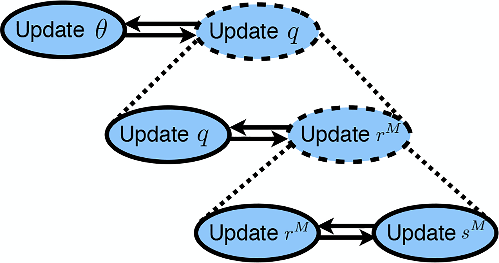
Illustration of optimization algorithm. Solid ovals denote closed-form update steps. Dashed ovals with dotted expansion lines denote updates that are implemented by alternating optimization. Pairs of opposing arrows indicate alternating optimization implemented by iterating each update to convergence. See the extended version (Libbrecht et al., 2015) for the full algorithm.

Theorem 2.4. The modified EM algorithm monotonically increases the relaxed EGPR objective:

$$J_{\text{EGPR}-\mathrm{R}2}\left({\theta }^{\left(t\right)}\right)\le J_{\text{EGPR}-\mathrm{R}2}\left({\theta }^{\left(t+1\right)}\right).$$ (20)

Proof: See extended version (Libbrecht et al., 2015).

3. EGPR for Inference

In addition to its use for regularized learning, EGPR can be used directly as an inference algorithm. To do this, we compute $q^{*}\leftarrow {\text{argmax}}_q{J}_{\text{EGPR-R2}}^{\prime }(\theta ,q)$ and use this distribution as the posterior. As discussed above, $q^{*}$ obeys the same factorization properties as $p_{\theta }$, so algorithms such as Viterbi and belief propagation can be used to compute the MAP solution and marginal distributions of $q$ respectively. Using EGPR as an inference algorithm results in posteriors which are smooth with respect to the graph $G_R$.

4. Related work

The most straightforward way to express similarity information in an unsupervised model is to encode it in the graphical model. For example, one might add a factor between $X_u$ and $X_v$ as in $\varphi \left(x_u,x_v\right)=\lambda 1\left(x_u=x_v\right)$. This form of interaction is quite different from EGPR, because adding factors changes the “implementation” of the model, while EGPR regularizes what the model does. Moreover, there are two problems with this approach. First, it is not always clear what form of interaction is most appropriate. In particular, although KL-based penalties have been very successful in graph-based semi-supervised learning, they cannot be converted to an equivalent set of probability factors. Second, adding similarity edges to the probabilistic model results in a model that does not, in general, have low tree-width, so efficient exact inference algorithms such as belief propagation cannot be used, and one must resort to approximate inference. As we show in Section 5.2, EGPR performs better than the loopy belief propagation (LBP) approximate inference algorithm on an augmented graph.

Three methods take a similar approach to ours, by augmenting a probabilistic model with a graph regularizer. First, Altun et al. (2005) describe a graph regularization for maxmargin models applied to pitch-accent prediction and optical character recognition. However, this method involves a matrix inversion step, and thus it cannot scale to large models. Second, Subramanya et al. (2010) combine a temporal conditional random field with a regularizer that expresses pairwise squared-error penalties derived from unlabeled data. They apply this method to the part-of-speech tagging task (Subramanya et al., 2010) and later to related problems in natural language (Das & Petrov, 2011; Das & Smith, 2011). That work, however, resorts to a purely heuristic update step and lacks any optimality guarantees.

Third, He et al. (2013) present an approach based on an exponentiated gradient descent algorithm. Like our approach, He’s approach exhibits monotone convergence. Although He’s work has many similarities with our approach, He’s work differs from ours in three important ways. First, He’s method uses a squared-error penalty, which, as argued above, is less appropriate for probability distributions than Kullback-Leibler divergence (Bishop, 1995, p. 226). As shown in Section 5.2, using squared error also results in worse performance in practice. Second, the exponentiated gradient descent method is applied to semi-supervised handwriting recognition and part-of-speech tagging, while we apply EGPR to an unsupervised genome annotation problem. Third, He et al. (He et al., 2013) use an exponentiated gradient descent strategy, while we use alternating optimization.

Our alternating optimization approach has several benefits over the exponentiated gradient descent method of He et al. (He et al., 2013). First, the He et al. algorithm involves gradient calculations over each clique in the conditional dependence graph, with order $O\left(k^{\left|C\right|}\right)$ for a variable of dimension $k$ involved in cliques of size $\left|C\right|$. Our alternating minimization algorithm, by contrast, has closed-form updates of order $O\left(k\right)$ for $q,r^M$ and $s^M$. (Updates for $\theta$ can still involve $O\left(k^{\left|C\right|}\right)$ calculations, but these are generally very fast). Therefore, the alternating optimization algorithm is more appropriate for extremely large models or models with large cliques or high-order factors. Second, empirical studies of KL-based graph smoothness objectives have shown that alternating optimization algorithms perform better than gradient-based methods for these objectives (Subramanya & Bilmes, 2011). Finally, the alternating optimization strategy is parallelizable and extremely simple to implement because the graph regularization step has simple, closed-form updates with no learning rate hyperparameters, and the posterior calculation can be performed using any probabilistic inference method on a model with the same conditional dependence graph as the unregularized model.

5. Simulations

In addition to the results shown below, in the supplement (Libbrecht et al., 2015), we show results for an application of EGPR to genome physical interactions on real and simulated data. All implementations in the below use the GMTK, the graphical models toolkit, and its use of virtual evidence factors, for HMM and dynamic graphical model inference

5.1. Learning a Gaussian Mixture on Poorly-Separated Data

First, we consider a simple example that demonstrates the utility of EGPR (Figure 2). Suppose we wish to learn a mixture of four Gaussians on data lying in a circle in 2D, using EM training to find cluster centers. Clearly, the training problem is underspecified in this case, because any set of centers at 90 degrees from one another relative to the circle’s center represents an optimum of the model likelihood. However, suppose we additionally have pairwise information that certain slices of the circle should form clusters. To represent this additional information, we form a regularization graph that connects all pairs of positions within the same cluster and run EM with EGPR using this graph. EGPR finds the true cluster centers and recovers the true labels with 100% accuracy compared to 74% accuracy with EM alone. This example demonstrates how pairwise information can be integrated in the training process to produce a trained model that implicitly incorporates this information.

Figure 2.

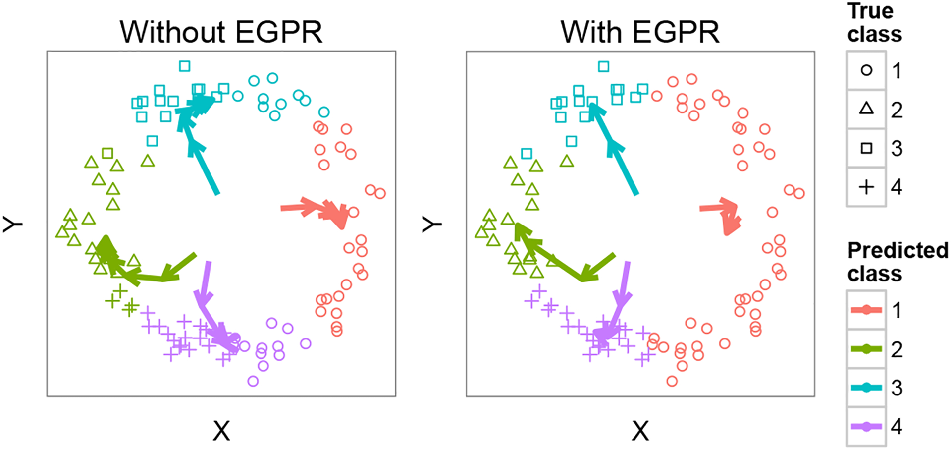
Using EGPR to learn ambiguous clusters. Shape denotes true class, color denotes predicted class, and colored arrows denote cluster means as they evolve between iterations of EM.

5.2. Comparison with Related Inference Methods

To evaluate the efficacy of EGPR, we compared EGPR to two related methods: 1) approximate inference on a graphical model with the same dependence structure, and 2) GPR using squared-error penalties. We compared to the approximate inference method loopy belief propagation (LBP) because it is one of the most widely used approximate inference methods. While we would have preferred to perform this comparison using our genomics data sets (see Section 6), due to the large size of the models and dense connectivity of the regularization graphs, it appeared that even our implementations of these methods would take months to converge. Therefore, we instead performed this comparison using synthetic data. We generated a chain of length $n=200$, with $\left(X_H,X_O\right)=\left(Z_{1:200},Y_{1:200}\right)$, where $Z_{1:200}\in \{\mathrm{0,1}{\}}^n$ and $Y_{1:200}\in {\mathbb{R}}^n$. We defined an HMM over this chain with transition probabilities $\text{PR}\left(Z_i=Z_{i+1}\right)=0.9$ and emission probabilities $Y_i~N\left(Z_i,\sigma \right)$, where we vary $\sigma$ to control the difficulty of the problem—higher $\sigma$ results in more challenging inference. We generated a graph $W\in {\mathbb{R}}^{n\times n}$ over the vertices of the chain by setting $w_{ij}=1$ with probability 0.4 if $Z_i=Z_j,w_{ij}=1$ with probability 0.1 if $Z_i\ne Z_j$, and $w_{ij}=0$ otherwise. This model is meant to simulate the task of labeling a chain (such as a genomic sequence) where we have noisy information about which pairs of positions have the same label.

We compared five methods of inference: 1) inference on each position independently, with no chain model; 2) inference on the chain alone, without using $W$; 3) LBP on the chain plus extra factors of $\text{PR}\left(X_i=X_j\right)=\text{sigmoid}\left(\lambda w_{ij}\right)$, where $\lambda$ controls the strength of these factors; 4) GPR using the regularization graph $W$ and a squared-error penalties as described in (He et al., 2013) (SQGPR); and 5) EGPR using the regularization graph $W$. We chose hyperparameters for each model (${\lambda }_G,{\lambda }_{\mathrm{R}1}$ and ${\lambda }_{\mathrm{R}2}$ for GPR and $\lambda$ for LBP) using a training set of 200 simulations. We evaluated results according to the average accuracy over 200 simulations of MAP inference on the model in question.

EGPR significantly outperforms all other models for all experiments (Figure 3, providing nearly as much improvement in accuracy as does the chain model itself. The pattern of accuracy is instructive in understanding the properties of each model. LBP performs very well when there is little noise, but becomes easily stuck in local optima on harder problems. GPR with squared error provides a modest improvement over the chain model, but has poor performance relative to KL penalties, consistent with previous work on semi-supervised methods (Subramanya & Bilmes, 2011).

Figure 3.

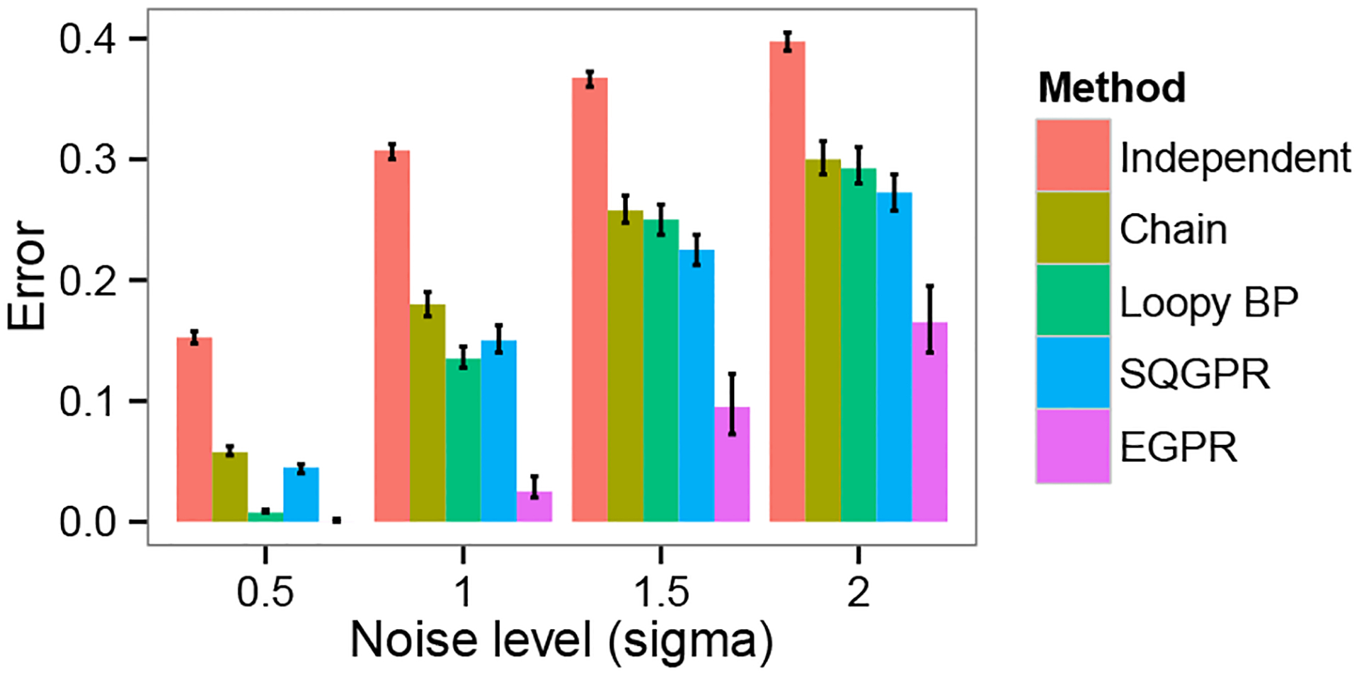
Comparison of EGPR with related inference methods. The X axis shows $\sigma$, a hyperparameter controlling the difficulty of inference. The Y axis shows the average accuracy over 200 simulations of MAP inference on the model in question (95% Wilcoxon test confidence intervals).

6. Application: Genome Annotation Using Physical Interaction Information

Recently, many methods have been described that partition and label the human genome on the basis of a number of genome-wide real-valued signal tracks, generally employing temporal models such as HMMs (Day et al., 2007; Hoffman et al., 2012a; Ernst & Kellis, 2010; Filion et al., 2010; Thurman et al., 2007; Lian et al., 2008). Formally, these methods aim to learn a labeling $X_{H1:n}\in \{1..L{\}}^n$ which associates each position in the genome with one of $L$ integer labels, such that positions that receive the same label exhibit similar patterns in the signal data. The input is comprised of a feature vector $X_{Oi}\in {\mathbb{R}}^F$ at each position that represents the output of biological experiments that measure local properties of the DNA, including its interaction with binding proteins, its local structure, and various types of chemical modifications. The process is “semi-automated” because a human assigns a semantic interpretation of the integer labels subsequent to the unsupervised learning phase.

However, existing genome annotation methods cannot incorporate the genome’s 3D conformation. The 3D arrangement of the genome in the nucleus plays a central role in gene regulation, chromatin state and replication timing (Misteli, 2007; Dekker et al., 2002; Ryba et al., 2010; Dixon et al., 2012). Genome conformation can be investigated using chromatin conformation capture experiments such as Hi-C (Lieberman-Aiden et al., 2009). A Hi-C experiment outputs a matrix of contact counts, where the number of contact counts of a pair of genomic positions is inversely proportional to the positions’ 3D distance in the nucleus (Lieberman-Aiden et al., 2009; Ay et al., 2014b). Existing genome annotation methods can incorporate any data set that can be represented as a vector defined linearly across the genome, but they cannot incorporate inherently pairwise Hi-C data without resorting to simplifying transformations such as principle component analysis.

We therefore present a novel strategy for integrating 3D conformation information using EGPR in which we encourage pairs of positions which interact in 3D to receive the same label in the annotation by connecting these positions with edges in an EGPR graph (Figure 5(a)). While the assumption that positions close in 3D space have similar regulatory state is not necessarily true at a small scale (~1 thousand base pair elements), it does generally hold at a large scale (~1 million base pair elements) (Lieberman-Aiden et al., 2009).

Figure 5.

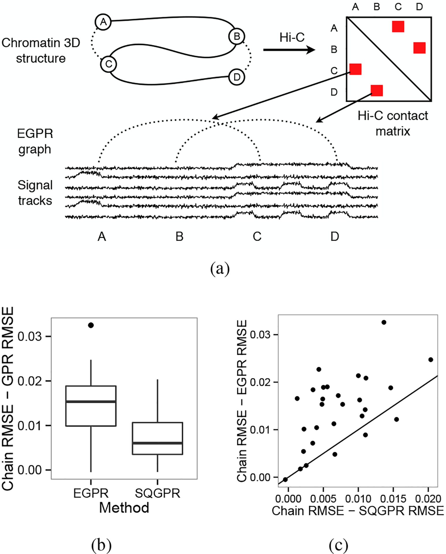
(a) Strategy for utilizing physical interaction information. (b) Improvement in RMSE over chain model for EGPR and SQGPR for 29 experiments. (c) Relative improvement in RMSE between EGPR and SQGPR for each of 29 experiments.

6.1. Synthetic Example

To motivate this approach, we first consider a simple synthetic model with 501 nodes and six EGPR edges. Let $Y_i\in \left\{\mathrm{0,1}\right\}$ for $i=0\dots 500$. We assign $Y_1=0$ and $Y_{500}=1$. Let $P\left(Y_{0:500}\right)={\prod }_{i=0}^{499}{0.9}^{1\left(Y_i=Y_{i+1}\right)}{0.1}^{1\left(Y_i\ne Y_{i+1}\right)}$. In other words, the model places higher probability on neighboring positions taking the same label but provides no other information. We construct an EGPR graph with $w_{\mathrm{0,200}}=w_{\mathrm{0,400}}=w_{\mathrm{200,400}}=w_{\mathrm{100,300}}=w_{\mathrm{100,500}}=w_{\mathrm{300,500}}=1$, corresponding to a hypothetical 2D arrangement of the chain. Without EGPR, the model learns a trivial labeling of the chain, whereas with EGPR, the model learns a labeling corresponding to the 2D arrangement (Figure 4).

Figure 4.

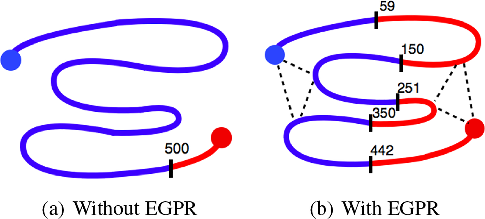
Synthetic model of genome spatial interactions. Color and labeled division lines indicate learned labels along the hypothesized 501 bp genome. Large filled circles indicate observed positions. Dotted lines indicate EGPR edges.

6.2. Real data

Next, to evaluate the efficacy of our approach, we performed genome annotation of the human fibroblast cell line IMR90. We compared three models: (1) the chain model described in (Hoffman et al., 2012a), without 3D structure data, (2) the chain model augmented with 3D structure data expressed with squared-error GPR (SQGPR), and (3) the chain model augmented with 3D structure data expressed with EGPR. We would have liked to compare against loopy belief propagation as well, but as mentioned previously, it appeared that our fastest implementation of this method would take months to converge on this large data set. In order to evaluate our performance in a variety of conditions, we ran each model separately once for each of the 29 available data sets in IMR90.

For SQGPR and EGPR, we used a GBR graph based on 3D structure data. To generate the GBR graph representation of 3D structure used by EGPR and SQGPR, we used the Hi-C data set of (Dixon et al., 2012) and processed the Hi-C data into a matrix of pairwise $p$-values using the Fit-Hi-C method (Ay et al., 2014a). To remove noise and decrease the degree of the graph, we removed all contacts with uncorrected p-value $p>{10}^{-6}$ and multiplied the remaining $p$-values by 10⁶, similar to a Bonferroni correction. We generated the GPR graph by setting the weight between positions $i$ and $j,w(i,j)$, to $w(i,j)\triangleq \text{max}\left(0,-{\text{log}}_e\left(p(i,j)/{10}^6\right)\right)$, where $p(i,j)$ is the $p$-value of interaction between positions $i$ and $j$. All annotations used four labels and binned the genome at 10,000 base pair resolution, comparable to the resolution of 40,000 bp used in (Dixon et al., 2012). We chose the best-performing hyperparameters for each GPR model using a validation set.

To evaluate these annotations, we used the time during the cell cycle at which the DNA is replicated as a gold standard (Woodfine et al., 2004). Replication time is highly correlated with gene expression and chromatin state and therefore is a good proxy for domain type (Lieberman-Aiden et al., 2009). To evaluate the accuracy with which an annotation predicts replication time, we compute a prediction as follows. Let $a_i\in \{1\dots 4\}$ and $x_i$ be the annotation label and replication time at position $i$, respectively. We compute the replication time mean over the positions assigned a given label $\ell$ as

$${\mu }_{\ell }\triangleq \frac{\sum _{i=1}^{n}1\left(a_i=\ell \right)x_i}{\sum _{i=1}^{n}1\left(a_i=\ell \right)}\text{for}\ell \in \{1\dots 4\}.$$ (21)

We define a predicted replication time vector $x_i^p={\mu }_{a_i}$ and compute the root mean squared error (RMSE) of this prediction as $\text{RMSE}=\sqrt{{\sum }_i{\left(x_i-x_i^p\right)}^2}$. EGPR consistently outperforms both the chain model alone and SQGPR (Figure 5).

References

- Altun Yasemin, Belkin Mikhail, and Mcallester David A. Maximum margin semi-supervised learning for structured variables. In NIPS, pp. 33–40, 2005. [Google Scholar]
- Ay F, Bailey TL, and Noble WS Statistical confidence estimation for Hi-C data reveals regulatory chromatin contacts. Genome Research, 24:999–1011, 2014a. [DOI] [PMC free article] [PubMed] [Google Scholar]
- Ay F, Bunnik EM, Varoquaux N, Bol SM, Prudhomme J, Vert J-P, Noble WS, and Le Roch KG Three-dimensional modeling of the P. falciparum genome during the erythrocytic cycle reveals a strong connection between genome architecture and gene expression. Genome Research, 24:974–988, 2014b. [DOI] [PMC free article] [PubMed] [Google Scholar]
- Bishop C Neural Networks for Pattern Recognition. Oxford UP, Oxford, UK, 1995. [Google Scholar]
- Chapelle O, Zien A, and Schölkopf B (eds.). Semi-supervised learning. MIT Press, 2006. [Google Scholar]
- Csiszár I and Tusnády G Information geometry and alternating minimization procedures. Statistics and decisions, pp. 205, 1984. [Google Scholar]
- Das D and Petrov S Unsupervised part-of-speech tagging with bilingual graph-based projections. In NAACL, pp. 600–609, 2011. [Google Scholar]
- Das D and Smith NA Semi-supervised framesemantic parsing for unknown predicates. In Proc. of ACL,2011. [Google Scholar]
- Day N, Hemmaplardh A, Thurman RE, Stamatoyannopoulos JA, and Noble WS Unsupervised segmentation of continuous genomic data. Bioinformatics, 23(11):1424–1426, 2007. [DOI] [PubMed] [Google Scholar]
- Dekker J, Rippe K, Dekker M, and Kleckner N Capturing chromosome conformation. Science, 295(5558): 1306–1311, 2002. [DOI] [PubMed] [Google Scholar]
- Dixon Jesse R, Selvaraj Siddarth, Yue Feng, Kim Audrey, Li Yan, Shen Yin, Hu Ming, Liu Jun S, and Ren Bing. Topological domains in mammalian genomes identified by analysis of chromatin interactions. Nature, 485(7398): 376–380, 2012. [DOI] [PMC free article] [PubMed] [Google Scholar]
- ENCODE Project Consortium. An integrated encyclopedia of DNA elements in the human genome. Nature, 489: 57–74, 2012. [DOI] [PMC free article] [PubMed] [Google Scholar]
- Ernst J and Kellis M Discovery and characterization of chromatin states for systematic annotation of the human genome. Nature Biotechnology, 28(8):817–825, 2010. [DOI] [PMC free article] [PubMed] [Google Scholar]
- Filion GJ et al. Systematic protein location mapping reveals five principal chromatin types in drosophila cells. Cell, 143(2):212–224, 2010. [DOI] [PMC free article] [PubMed] [Google Scholar]
- Ganchev K, Graça J, Gillenwater J, and Taskar B Posterior regularization for structured latent variable models. Journal of Machine Learning Research, 11:2001–2049, 2010. [Google Scholar]
- He Luheng, Gillenwater Jennifer, and Taskar Ben. Graph-based posterior regularization for semi-supervised structured prediction. In CoNLL, 2013. [Google Scholar]
- Hoffman MM, Buske OJ, Wang J, Weng Z, Bilmes JA, and Noble WS Unsupervised pattern discovery in human chromatin structure through genomic segmentation. Nature Methods, 9(5):473–476, 2012a. [DOI] [PMC free article] [PubMed] [Google Scholar]
- Hoffman MM et al. Integrative annotation of chromatin elements from ENCODE data. Nucleic Acids Research, 41(2):827–41, 2012b. [DOI] [PMC free article] [PubMed] [Google Scholar]
- Joachims T Transductive inference for text classification using support vector machines. In ICML, pp. 200–209, 1999. [Google Scholar]
- Lian H, Thompson W, Thurman RE, Stamatoyannopoulos JA, Noble WS, and Lawrence C Automated mapping of large-scale chromatin structure in encode. Bioinformatics, 24(17):1911–1916, 2008. [DOI] [PMC free article] [PubMed] [Google Scholar]
- Libbrecht Maxwell W, Hoffman Michael M, Bilmes Jeffrey A, and Noble William S. Entropic graph-based posterior regularization: Extended version. Proceedings of the International Conference on Machine Learning, 2015. [PMC free article] [PubMed] [Google Scholar]
- Lieberman-Aiden Erez, van Berkum Nynke L, Williams Louise, Imakaev Maxim, Ragoczy Tobias, Telling Agnes, Amit Ido, Lajoie Bryan R, Sabo Peter J, Dorschner Michael O, et al. Comprehensive mapping of long-range interactions reveals folding principles of the human genome. Science, 326(5950):289–293, 2009. [DOI] [PMC free article] [PubMed] [Google Scholar]
- Misteli T Beyond the sequence: Cellular organization of genome function. Cell, 128(4):787–800, 2007. [DOI] [PubMed] [Google Scholar]
- Neal RM and Hinton GE A view of the EM algorithm that justifies incremental, sparse, and other variants. In Learning in graphical models, pp. 355–368. MIT Press, 1999. [Google Scholar]
- Ryba Tyrone, Hiratani Ichiro, Lu Junjie, Itoh Mari, Kulik Michael, Zhang Jinfeng, Schulz Thomas C, Robins Allan J, Dalton Stephen, and Gilbert David M. Evolutionarily conserved replication timing profiles predict long-range chromatin interactions and distinguish closely related cell types. Genome research, 20(6):761–770, 2010. [DOI] [PMC free article] [PubMed] [Google Scholar]
- Subramanya A and Bilmes J Semi-supervised learning with measure propagation. Journal of Machine Learning Research, 12(10):33113370, November 2011. [Google Scholar]
- Subramanya A, Petrov S, and Pereira F Efficient graph-based semi-supervised learning of structured tagging models. In Proc. of EMLNP 2010, pp. 167–176. Assoc. for Comp. Linguistics, 2010. [Google Scholar]
- Thurman Robert E, Day Nathan, Noble William S, and Stamatoyannopoulos John A. Identification of higher-order functional domains in the human encode regions. Genome Research, 17:917–927, 2007. [DOI] [PMC free article] [PubMed] [Google Scholar]
- Wang Jun, Jebara Tony, and Chang Shih-Fu. Graph transduction via alternating minimization. In Proceedings of the 25th international conference on Machine learning, pp. 1144–1151. ACM, 2008. [Google Scholar]
- Woodfine K, Fiegler H, Beare DM, Collins JE, McCann OT, Young BD, Debernardi S, Mott R, Dunham I, and Carter NP Replication timing of the human genome. Human molecular genetics, 13(2):191–202, 2004. [DOI] [PubMed] [Google Scholar]
- Zhu Xiaojin and Ghahramani Zoubin. Learning from labeled and unlabeled data with label propagation. Technical report, 2002. [Google Scholar]
- Zhu Xiaojin, Kandola Jaz S, Ghahramani Zoubin, and Lafferty John D. Nonparametric transforms of graph kernels for semi-supervised learning. In NIPS, volume 17, pp. 1641–1648, 2004. [Google Scholar]
Associated Data
This section collects any data citations, data availability statements, or supplementary materials included in this article.