

Abstract
One of the leading causes of death for women worldwide is breast cancer. Early detection and prompt treatment can reduce the risk of breast cancer-related death. Cloud computing and machine learning are crucial for disease diagnosis today, but they are especially important for those who live in distant places with poor access to healthcare. While machine learning-based diagnosis tools act as primary readers and aid radiologists in correctly diagnosing diseases, cloud-based technology can also assist remote diagnostics and telemedicine services. The promise of techniques based on Artificial Neural Networks (ANN) for sickness diagnosis has attracted the attention of several re-searchers. The 4 methods for the proposed research include preprocessing, feature extraction, and classification. A Smart Window Vestige Deletion (SWVD) technique is initially suggested for preprocessing. It consists of Savitzky-Golay (S-G) smoothing, updated 2-stage filtering, and adaptive time window division. This technique separates each channel into multiple time periods by adaptively pre-analyzing its specificity. On each window, an altered 2-stage filtering process is then used to retrieve some tumor information. After applying S-G smoothing and integrating the broken time sequences, the process is complete. In order to deliver effective feature extraction, the Deep Residual based Multiclass for architecture (DRMFA) is used. In histological photos, identify characteristics at the cellular and tissue levels in both tiny and large size patches. Finally, a fresh customized strategy that combines a better crow forage-ELM. Deep learning and the Extreme Learning Machine (ELM) are concepts that have been developed (ACF-ELM). When it comes to diagnosing ailments, the cloud-based ELM performs similarly to certain cutting-edge technology. The cloud-based ELM approach beats alternative solutions, according to the DDSM and INbreast dataset results. Significant experimental results show that the accuracy for data inputs is 0.9845, the precision is 0.96, the recall is 0.94, and the F1 score is 0.95.
Keywords: Remote diagnostics, smart window vestige deletion, deep residual based multiclass for feature extraction approach, ameliorate crow forage-ELM
Introduction
During the course of their lifetime, 1 in 9 women will acquire breast cancer, which is a dangerous condition. Studies show that 1 in 32 women would be recognized as having breast cancer and die from it. Around 1 out of 4 recently discovered cancers in women, making it the most common type of new cancer diagnoses. Breast cancer is the 17th greatest mortality rate worldwide and the main danger factors for cancer in women. It is the third-most prevalent type of cancer in women aged 50 to 59, while being the most common malignancy in those aged 15 to 49. 1 Often known as a cancer that destroys healthy cells, aberrant human cell development. Breast cells that are growing abnormally will infiltrate nearby cells more quickly and spread to other bodily regions. Breast tumors (masses of tissue) that are malignant develop into breast cancer. Non-cancerous or benign and cancerous or malignant breast cancer are the 2 types.2,3 Ref. 1 or, Ref.2,3 or Ref.4-6 See the end of the document for further details on references.
Early-stage research on breast cancer have shown that small-scale weight loss is safe and useful,4,5 and trials are still ongoing to determine the impact on survival. 6 There is still a need to comprehend how weight loss affects a wider range of out-comes, including body composition, 7 the risk of developing chronic diseases, and patient-reported outcomes, such as quality of life and side effects from therapy. Fatigue, arthralgia, and menopausal symptoms are a few treatment-related adverse effects that might last a long time 8 and are made worse by being overweight. 9 Few trials have investigated how weight reduction affects patients’ studies in the past, with the exception of quality of life. Moreover, studies on weight loss have primarily examined effects on specific metabolic indicators; wider assessments of chronic disease risk.
Applications for cloud computing have drawn a lot of interest over the past few years because of their less expensive acquisition prices. Data may be connected into the cloud thanks to its web application, which enables IT personnel to access all of their computer resources from anywhere. 10 Moreover, cloud computing provides a wealth of tools for processing and storing large collections of medical pictures.11,12 Via a dashboard, a web-based tool provided by cloud computing, IT staff members have the ability to use the cloud support company’s. Since cloud computing is suited for integrating data saved on the cloud, updating medical records has become simpler. Many services offered by cloud computing enable the healthcare sector to operate more reliably and with less downtime. 13 Numerous patients struggle with a short-age of facilities, but thanks to cloud computing, doctors can diagnose them and provide tele-health 14 and telemedicine, which involves sending different medical data, like video tapes and higher healthcare images of service users, from remote locations to other places with access to doctors. However, many of them do not advance to the pre-clinical level and require further investigation. The device’s ability to identify breast tumors is mostly determined by skin reflection and antenna coupling. Clutter removal techniques can reveal disguised internal responses. The averaging procedure is usually straightforward and effective. 15 Although adequate for idealized conditions, the outcomes may not meet expectations in complex scenarios. Back scattered signals may exhibit modest spatial vibrations due to system jitter and external interference. Applying this approach across the entire time series will result in additional replies and lower image quality.
To fix the problem, this study suggests an automated system that uses a methodical approach to detect breast cancer. DDSM and INbreast dataset provided the in-formation. An adaptively splitting backscattered signals into several temporal windows (either with equal or unequal intervals) is done using the Smart Window Vestige Deletion (SWVD) method. This approach analyzes backscattered signals and divides them into time windows (equal or uneven intervals) adaptively. The altered 2-stage filtering procedure is applied to each window to remove irrelevant responses. After processing all windows, signals are combined to complete the sequence. Then Savitzky-Golay (S-G) adaptive filtering is used to reduce small sounds. Deep residual based multiclass for feature extraction approach (DRMFA) architecture to provide efficient feature extraction. Extract characteristics at the cellular and tissue levels from both smaller and bigger size patches in histology images. Following that, the Ameliorate Crow Forage-ELM method is used to identify and classify micro calcification in digital pictures. The primary goals of the planned effort are to accurately detect breast cancer and categories its severity (benign or malignant severity).
The contribution of this research is
A window based updated 2 stage filtering and savitzkyGolay(S-G) method is proposed. The Savitzky-Golay filter is a digital filter used for data smoothing.
Savitzky-Golay (S-G) smoothing, updated 2-stage filtering, and intelligent temporal window division are all part of a revolutionary pre-processing method.
The Smart window vestige deletion has the best results for reducing unnecessary reflections, clearing up huddle, and enhancing rebuilt images.
The rest of this essay; Section 3 provides a description of the technique utilized in this work; Section 4 discusses the various findings of this study; and Section 5 discusses the conclusions and suggested directions for further research.
Literature Survey
Many researchers are interested in the diagnosis of breast cancer diseases. We go over a couple of the diagnostic testing methods below. Our integrated techniques for distinguishing between typical malignant lesions and aggressive cancer, we developed a nested ensemble strategy that combined the classifiers stacking and voting (voting). a fresh hybrid ensemble strategy to enhance breast cancer classification algorithms for early detection. K-fold cross validation (K-CV) was used in the study to test the efficacy of hybrid ensemble methods in this circumstance. A 98.07% accuracy was achieved by the SV-BayesNet-3-MetaClassifier and the SV-Nave Bayes-3-MetaClassifier (K = 10). However, SV-Nave Bayes-3-MetaClassifier performs better. 16 Because it develops the model more quickly. Transfer learning for the identification of breast cancer. The revised VGG (MVGG) is developed using datasets of mammograms in 2D and 3D. The suggested according to experiment results. The mathematical threshold value is significantly higher than the threshold value utilized for clinical classification. By using this method, the incidence of false-negative mammography cases will be greatly reduced. 17
The main goal of this framework is to develop a for the detection of breast cancer by combining the method with the fruit fly optimization algorithm (FOA) to enhance 2 crucial SVM characteristics. The volunteer high-level characteristics are used to make the initial diagnosis of breast cancer. The effectiveness of the suggested method is compared to that of current models, such as the LFOA-SVM is the combination of FOA and LF method, which raises the quality of FOA, speeds up the pace of convergence, and lowers the possibility of eluding the local optimal solution. 18
The Wisconsin Diagnostic Breast Cancer (WDBC) Dataset was subjected to SVM (with a radial basis kernel), ANNs, and Naive Bayes. This study is about integrating several ml models algorithms with a choice of methods for extracting features and evaluating the outcomes in order to pick the optimum line of action. The goal is to combine the advantages of background subtraction and computer vision. By employing Linear Discriminant Analysis (LDA) to decrease the high dimensionality of the da-ta and then using SVM to the new reduced feature dataset, this study offered a hybrid strategy for the detection of breast cancer. Results were 99.07% specificity, 98.41% sensitivity, 98.82% accuracy, and 0.9994 area under the receiver operating characteristic curve when the proposed method was used. 19 The classification of hematoxylin and eosin stain (H&E) histological breast cancer photos was requested by the International Conference on Image Analysis and Recognition (ICIAR) 2018 Grand Challenge on Breast Cancer Histology (BACH) Images. To extract descriptive information, the technique combined a pooling layer with a Deep Convolutional Neural Network (DCNN) model. Deeplearning is its foundation, and it is completely autonomous. To improve DCNN performances, a number of data enhancement approaches are used.
A pre-trained Xception model produces categorization results with an average accuracy of 92.50%. 20 a meta-heuristic method for configuring the neural network. By combining a wavelet neural network (WNN) with a gray wolf optimization (GWO) method, the primary outcome of this research is the creation of a desktop diagnosis method for detecting abnormal in ultrasound images pictures. Here, a sigmoid filter, anisotropic diffusion, and interference-based despeckling are used as data preprocessing on breast ultrasound (US) pictures. Using the automated segmentation method, the target area is collected, and then morphology and textural features are computed. Lastly, the classification process is accomplished by utilizing the GWO tuned WNN. Better accuracy is provided (98%) by the proposed GWO-WNN method. 21 Develop and assess miRNA sets which are suitable for breast cancer early detection. Nine possible miRNA biomarkers were selected by looking at references miRNAs related to the development and advancement of breast cancer in an effort to identify unique miR-NAs that may be used to diagnosis early breast cancer. Using the trained cohort, a set of miRNAs that could be utilized to identify breast cancer were discovered. This miRNA variation was validated using the testing cohort. The samples that were collected were used to receive the full RNAs. Reverse transcription analytical PCR was used to measure the amounts of 9 miRNAs. Nine candidate miRNA levels in healthy individuals and breast cancer patients were examined. Detecting breast cancer with a combination of 4 miRNAs has a 98% sensitivity, 96% specificity, and 97% accuracy in the validation cohort. 22
Black-box techniques that are unable to identify the causes of the diagnose. The term “enhanced Random Forest (RF)-based rule extraction” refers to a technique for generating accurate and understandable classification model from a decision tree ensemble for the cancer detection process (IRFRE). Many decision tree models are first built using Random Forest in order to create a large number of decision rules. After-wards when, a technique is developed for generating decision tree from the training trees. An updated multi-objective algorithm (MOEA) is used to determine the best rules prediction, and the element rules set reflects the best compromise among accuracy and interpretability. 23 The operation and structure of each network are investigated in detail, and the precision with which every network diagnoses and classifies breast cancer is then analyzed to find which system operates considerably better. Ac-cording to reports, CNN is marginally more accurate than MLP for the identification and diagnosis of breast cancer. 24
A cutting-edge deep learning system is used to identify and categories breast cancer in breast cytology images utilizing the concept of transfer learning. Deep learning systems are employed regularly on their own. Transfer learning, as opposed to traditional learning models that build and generate in isolation, tries to apply the information gained when solving one difficulty to another that is related. The suggested method extracts feature from images using pre-trained CNN architectures like Goog-LeNet, Visual Geometry Group Network (VGGNet), and Residual Networks (ResNet). These designs are then utilized to categorize benign and malignant cells using average pooling classification, employing a fully linked layer. 25 To calculate the range-based cancer score, the Breast Cancer Surveillance Consortium (BCSC) dataset is used and updated using a proposed probabilistic model. The proposed model examines a subset of the total BCSC dataset, which includes 67 632 records and 13 risk factors. Three sorts of data are collected: general cancer and non-cancer probability, prior medical information, and the likelihood of each risk factor given all prediction classes. The model also use weighting methodology to create the most effective fusion of the BCSC’s risk criteria. The final prediction score is calculated using the post probability of a weighted mix of risk factors and the 3 statistics obtained from the probabilistic model. 26
To address the challenge of detecting early-stage breast cancer, we present a medical IoT-based diagnostic system that can competently distinguish between malignant and benign people in an IoT environment. For malignant versus benign classification, the artificial neural network (ANN) and convolutional neural network (CNN) with hyper parameter optimization are used, with the Support Vector Machine (SVM) and Multilayer Perceptron (MLP) serving as baseline classifiers for comparison. Hyper parameters are vital for machine learning algorithms because they directly regulate training algorithm behavior and have a major impact on model performance. 27
In recent years, deep-learning (DL) techniques have proven to be extremely effective in a range of medical imaging applications, including histopathology pictures. The goal of this study is to regain the identification of BC using deep learning techniques by combining qualitative and quantitative data. This study focused on BC through deep mutual learning (DML). In addition, a wide range of breast cancer imaging modalities were studied to determine the difference between aggressive and benign BC. Deep convolutional neural networks (DCNNs) have been developed to evaluate histopathology pictures of BC. The DML model attained accuracy levels of 98.97%, 96.78, and 96.34 respectively. 28
Backscattered signals may exhibit modest spatial vibrations due to system jitter and external interference. Applying this approach across the entire time series will result in additional replies and lower image quality.
Proposed Method
The creation of a cloud-based breast cancer diagnosis platform is suggested in this paper, along with the provision of remote user health data monitoring. The technology is adaptable enough to identify and categorize a range of ailments while analyzing consumer health data stored on cloud servers. However, in this research, we mainly concentrated on a single application—categorizing diseases as “cancerous” or “non-cancerous.” The general design of the architecture that we propose is shown in Figure 1. The patient visits the remote health care in their region that is a part of the suggested architecture, where the health-care source gathers the patient’s data, including x-rays and other health metrics, and delivers it to a doctor through the Internet.
Figure 1.

Proposed architecture.
Three phases of processing take place in the cloud. Initially, a preprocessing method called Smart window vestige deletion (SWVD) is suggested. It includes Savitzky-Golay (S-G) smoothing, updated 2-stage filtering, and intelligent temporal window division. Next, in order to deliver effective feature extraction, Deep residual based multiclass for feature extraction approach (DRMFA) architecture to provide efficient feature extraction. Extract characteristics at the cellular and tissue levels from both smaller and bigger size patches in histology images. Last but not least, a novel customized technique has been created that makes use of an Ameliorate Crow Forage-ELM and combines the concept of deep learning with the extreme learning mechanism (ELM).
Smart window vestige deletion (SWVD) approach
The weight vector w is only estimated using data from the artifact interval in the TSR approach. W is involved throughout the entire time series once the clutter has been removed. As a result, if this parameter and other parts are mismatched, redundant information could be introduced. This would seriously interfere with the imaging step. The suggested SWVD method can minimize irrelevant responses, which lowers noise and improves the confocal image. The 3 phases of this method are S-G smoothing, modified 2-stage filtering, and adaptive time window division. Contrary to popular belief, the weight vector is not taken into account for the entire sequence. It executes numerous calculations with a smaller sampling scale. Because of this, each window’s w solutions are more flexible, and redundant information is reduced. As a result, the region of interest (ROI) in confocal images can be enhanced and interference areas can be reduced. Algorithm 1 shows the pseudo code.
The basic time window in adaptive window division, which consists of the artifact region and the target region, has a length known as . The magnitude of the huddle is initially determined by looking at the peak of the align and normalized channel signals. In order to prevent the anticipated information from being incorrectly suppressed, it is also required to provide a proper range behind the artifact because the tumor response is frequently close to the artifact. The base window then travels in a non-superposition direction toward both ends. It can be accepted as a fresh brief or blended through into previous window when an un allocated sequence has a span that is smaller than . This will result in certain adjusted windows’ lengths being different from those of their original windows ( ). The huddle and target regions’ ranges will be adjusted using the formula where the ratio is the ratio of the huddle’s scale to As a result, there may be variations in 1 channel’s time window size and number of split segments across different channels. Equation (1) can be used to describe the subsequent procedures:
| (1) |
where the t-th window’s sampling points are represented by the string The k-th channel’s segmented and entire raw signals are and . The window’s total number and order are t and T. and are the beginning and ending nodes of the artifact in The notation stands for the target region’s length within t-th segment of the divided sequence.
Then each stage of the altered 2-stage filtering is used to suppress huddle. In order to determine signal similarity, the correlation coefficient is initially used among the i-th and j-th angle, in the t-th window of the k-th channel. The first M-signals in each window that are greater than a predetermined threshold are added to a subset called and the rest are rejected.
If the quantity of needs by this threshold is less than M, all signals are processed. It must be noticed that the i-th angular signal’s neighboring signals are not considered while deciding . The is used to filter adaptively in the second stage. were represents a single signal that was chosen from the subset of . The following is the huddle removal principle:
| (2) |
Following the elimination of the artifact, the anticipated internal reflections in the t-th window are indicated by . The key to the entire strategy is , which represents the filter’s weight vector. A column vector is defined as follows to precisely obtain its optimal solution:
| (3) |
where L is the clutter interval, which contains all the information that needs to be hidden. Following that, a matrix is built based on each subset. The equation represents the relationship between the variables and weight . The weight vector is successfully solved by converting this equation into a generic minimal square form ( ) and adding a prior constraint with signal similarities. The weight vector is successfully solved by converting these equations into a generic minimal square form ( ) and adding a prior constraint with signal similarities. Thus, the following is the cost function:
| (4) |
and is the constraint parameter. It might be interpreted as looking for the best answers close to . The weight vector is finally expressed as: by minimising another equivalent equation (4).
| (5) |
In each window, this phase views some information as huddle The is used to eliminate these surprising responses when there are genuine artifacts. After window change, the weight vector will be recovered. As a result, each operation is completed independently. The procedure is comparable to mean filtering if signals vary somewhat in some regions. Following analysis of each segment, the backscattered signals are combined as follows:
| (6) |
where is the recovered sequence. Lastly, additional noise is eliminated using the S-G adaptive filtering. This method keeps both the maxima and minima while retaining the sharp edge’s sensitivity. The primary trend can be precisely extracted at the same time. Polynomial least square fitting, which is denoted as the following, might further suppress other responses:
| (7) |
where is the signal to be processed and is the denoised signal. The smoothing window’s smoothing factor, or , has a size of
Deep residual based multiclass for feature extraction approach
The following is a concise summary of the key processes: (i) In order to maintain important details and contain features at the cell and tissue levels, we employ a sliding window technique for obtaining various sizes of images the histology of breast cancer showing many sorts of patches. Then, we train 2 CNNs—one for each patch type—as feature extractors. (ii) Using the k-means clustering method, we separate the small patches into several groups and select more racist and discriminatory patches in order to teach the networking again. (iii) Using feature extractors, to construct the final feature of each image, extracted features from larger and lesser selected patches.
Sampling patches
The breast histology image will be divided into 4 categories: benign tissue, invasive cancer, in situ malignancy, and healthy tissue. The information gleaned from the photos has a significant impact on categorization performance. To depict each complete image, we employ breast cell-related features as well as general tissue components. Nuclei data, such as size and variation, in addition to organizational issues of cells, such as density and morphology, are examples of traits found at the cellular level are utilized to identify malignant cells. This is because malignant cells exhibit a typia, such as bigger nuclei and irregular shape, and because their arrangement is incredibly disorganized. The breast histology photos in the collection have pixels that are in size, and the cell radius is roughly between 3 and 11 pixels. Thus, to obtain cell-level characteristics, we take out little 128 × 128-pixel patches. Second, the diseased tissue might be structurally unique. In situ carcinoma is the term for the development of reduced malignant or premalignant cell within a specific tissue compartment, like the axillary duct, without invading of interstitium. Invasive cancer can expand outside of the initial tissue compartment as well. Differentiating among in situ and metastatic carcinoma cells requires an understanding of tissue architecture. A huge histology image cannot be directly used by CNNs to retrieve attributes. According to the dimensions of the images in the image net, of 512512 pixels to hold the data on the overall tissue architecture. We use a sliding window technique to extract patches of histopathology images. Despite the patches’ small size of 128 by 128 pixels, we extract continuous, and concentrate on cell-related characteristics. Also, they extract patches of 512 pixels × 512 pixels with 50% overlaps that contain categorical variables on the shape and architecture of the tissue. The label assigned to each extracted patch matches that of the relevant histological image.
Feature extractor
The histology images differ in terms of cell form, texture, tissue architecture, and other elements. The categorization process depends on the accurate representation of complex traits. The handmade approach to feature extraction is labor-intensive and challenging to extract discriminative features since it necessitates extensive specialist subject expertise. CNNs have produced outstanding results in a number of disciplines and can instantly extract representative characteristics from images. Even though ResNet50 is a normal CNN and simpler to train than some, it was chosen as the feature extractor in this study. This was done to ensure the extraction of usability features.
The deep residual learning framework (ResNet) is to deal with the deep network damage. Strictly speaking, the initial mapping is represented as , Then, a new mapping is fitted to the stacked nonlinear layers after the appropriate underneath mapping, has been determined that is . The identity mapping is performed by “shortcut connections.” A design is suggested for deeper nets that uses a stack of 3 layers rather than 2 for each residual function Figure 2A {3, 224, 224} RGB image is fed into the 16 building pieces that make up the ResNet50. In order to prevent over fitting, ResNet50 must be trained using a lot of training pictures. We employ ResNet50, which has already been trained on the Wisconsin Diagnostic Breast Cancer (WBCD) dataset, using a transfer learning methodology despite the fact that our dataset doesn’t contain many histology pictures. Before. ResNet50-512 and ResNet50-128 are the subsequently assigned names for the trained networks. The Global Average Pooling layer of ResNet50 can be used to extract 2048-dimensional features of patches.
Figure 2.
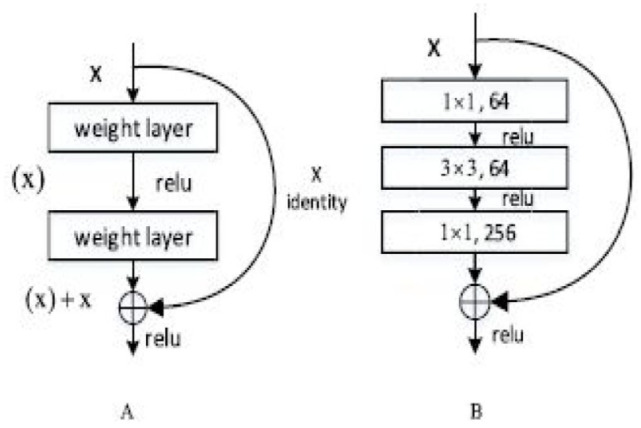
(A) A building block. (B) A bottleneck building block for ResNet50.
Screening patches
For selecting patches from histology images is laid forth. This section’s goal is to offer a technique for screening discriminative 128 × 128-pixel patches using ResNet50-128 and a few machine learning techniques.
Clustering: The 128 × 128-pixel patches could not have enough diagnostic data. For instance, there will be normal patches taken from images with malignant histology as well as patches with significant amounts of fat cells and stroma. In order to determine whether the breast cells are malignant, we want to choose discriminative patches that are labeled similarly to the source pictures and contain a sufficient number of breast cells. Batch-wise screening of racist and discriminatory patches, divide the patches into various groups based on their phenotypes. Row pixels are concatenated to create 1024-dimensional features, and patches of 128 pixels × 128 pixels are downscaled to create thumbnail images that are 32 pixels × 32 pixels in size. The 200 components of the patches are then preserved using principal component analysis (PCA), allowing us to illustrate their phenotypes before the K-means method. Following clustering, we obtain K distinct phenotypic groupings.
Selecting Clusters: Patches with distinctive characteristics are included in the candidate clusters found using K-means. Screen clusters using the to identify clusters with higher racist and discriminatory patch. The ResNet50-128 is more sensitive to these little patches because the majority of them show identical rich phenotypes that were derived from histological images that have the identical label. We use ResNet50-128 to forecast all of the patches in each cluster in order to identify the top k cluster the best categorization results, or cluster with is racist and discriminatory patches. After the ResNet50-128 has been retrained using the patch in the chosen clusters, the network with the updated weights is referred to as the ResNet50-cluster. This network can extract more representative features because it was trained using patches that included highly discriminative data.
Extreme learning machines
The ELM of the Single-Hided-Layer Feed-Forward Neural Networks (SLFN) class is a straightforward and effective learning method that seeks to reduce time and resources used on meaningless training while also enhancing generalization capability. The buried layer of the ELM does not require tuning. In other words, the input layer and hidden layer’s hidden neurons, biases, and weight vector of the SLFN are created at random and without further change. Also, the efficient least squares approach is use to choose the weights for the connections among the output layer and hidden layer. Figure 3 depicts the ELM’s structural layout.
Figure 3.
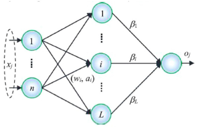
Extreme learning machine’s structure.
The output function of ELM is as equation (8).
| (8) |
where is a vector of output weights between the output nodes and the hidden layer with nodes. Moreover, the output vector of the hidden layer in relation to the input is . The data from the d-dimensional input space is actually mapped by to the L-dimensional hidden layer feature space H. The ELM decision function is as equation for applications involving binary classification (9).
| (9) |
In contrast to conventional learning algorithms, ELM aims to obtain not just the limited training errors but also the lowest norms of output weight, improving network performance (such as the BP algorithm).
| (10) |
| (11) |
The output weight can be defined as equation (12) if the desired matrix consists of labeled samples.
| (12) |
is the generalised Moore-Penrose inverse of matrix H. The ELM output layer functions as a linear solver in the new feature space H, and the only system parameters that need to be adjusted and are theoretically definable using equation (12).
Crow-search optimization algorithm (CSOA)
Crowd-search optimization is used in the job as a result because of its benefits of simpler and minimal parameter tuning. Many optimization techniques typically fail because of the significant disadvantage of having to tune additional parameters, which increases the time required for the process. The algorithm was naturally developed using crows as a model. when they are looking for food. The method is based on the following tenets.
(i) Each crow is taken to be a member of the flock.
(ii) Every crow can remember where their prey was buried.
(iii)Every crow in the flock can locate its other members and steal the food that is hidden.
(iv)With some likelihood, every crow in the flock is good at defending their food from outsiders.
Let’s assume that the flock size in a D-dimensional environment is . Taking into account that denotes the jth crow point in the search space at iteration, where j has values of 1, 2, 3,. . ..M. The given maximum number of iteration is also included. by . Every crow can readily recall their buried food, as stated in the CSOA principles, and is depicted as a hiding location for crows to titerate. Nj, t also indicates the best position attained by crows. A crow starts to locate the location of food that was hidden by another crow (z) at 1 iteration (t). Two scenarios are now possible:
Crow is monitoring the crow , who is unaware that it is being fed. As a result, the crow jnow moves closer to the location of the crow z’s hidden food. This updates the position of the crow as.
| (13) |
represents a randomly generated, even number between [0, 1], where is the flight duration of the crow jat iteration. The algorithm’s ability to search depends significantly on the value of ; a lower flvalue allows for local search while a greater value allows for global search.
The crow is aware that another crow is keeping tabs on its food. The crow will therefore lie about where it is in the search area in order to avoid the location of its food from being discovered. Combining the aforementioned scenarios mathematically and rendered as
| (14) |
Where is a random number between 0 and 1, distributed randomly and is the awareness probability of the zthcrow at the threshold, respectively. Exploitation (intensification) and exploration, the 2 primary parts of optimization, will be balanced here by the parameter AP (diversification). Smaller AP values typically influence intensification (enabling local search), while larger AP values typically impact diversification (allowing worldwide search).
The initial parameter settings for the crow-search algorithm are and values. The value of denotes is initialized at random and represents where each crow is located in the search space (as provided in equation (13)). The other crow in the group start to cover their catch in place N as the first crow in the group first struggles to conceal its food. When the algorithm is running, each crow’s location is evaluated using a fitness function. Now that the fitness value as depicted in equation has been determined, the crows can adjust their present places accordingly (13). The viability of the newly updated positions is constantly examined. As a result, the flock of crows can refresh their memory and express themselves as
| (15) |
where Fn(.) stands for the algorithm’s objective function.
Last but not least, the crow-search optimization algorithm’s process can be summed up as follows:
Flock size (M), the number of iterations allowed flight length and awareness probability are the first parameters selected
Random location and memory initialization in a search space of D dimensions.
To determine the fitness value, each crow’s posture is assessed.
In order to identify where its hidden prey is the crow moves to a different location, picks a random flock member ( ), and follows it.
Each crow in the flock will have its newly found location examined to determine whether it is practical its location will be updated. The location of the crow remains otherwise unchanged.
Fitness calculations for the new jobs that are practical.
Update the memory of crows based on equation (14).
Once the procedure has reached the required number of termination criteria (maximum iterations), stop it; otherwise, continue steps 4 through 7 until x is reached.
Ameliorate crow forage-ELM (ACF-ELM)
A few parameters must be randomly allocated for the majority of metaheuristic optimization strategies, either using a uniform or Gaussian distribution. As a result, either the optimization process is inconsistent or the rate of convergence is slower. Consequently, to address this problem, CSOA must be altered in 2 ways to speed up convergence. The method now has a simple control parameter that tells the flock of crows to search for global minima instead of local optima, which is the first modification. The next approach uses chaotic maps to control algorithmic unpredictable behavior for dependable and improved performance.
Making a control operator a part of the algorithm: Due to the fact that each crow in the flock chooses a different crow to follow as a leader, the updating of locations is carried out using equation (13). This proves that the likelihood of selecting any crow as the leader has a range of and is equal for ithcrow. It is obvious in this instance that not each M crow in the flocks has an identical probability because of the objective function. In order to optimize the algorithm, a control operator is built, which allows the crow to hunt for optimal solutions. This can be done by ranking and sorting all of the crows’ goal function values throughout each cycle. Ultimately, in its succeeding generation, mLastcrows are dropped from the optimization procedure by,
| (16) |
where gives the proportion of crows who were ejected from the flock at and gives the number of eliminated birds at titration in the starting population. It is clear from equation (9) that the time-dependent variable mLast fluctuates. Now that every crow is acknowledged as a leadership, making it simple for the flock to keep track of them. The number of crows will gradually decrease in the next iterations, and in the final iteration , there will only be crows left, allowing the optimization process to continue. This causes the algorithm to quickly search for global optima while escaping local optima. However, the randomness must still be controlled in order to improve its consistency and rate of convergence. This is covered in the next subsection.
Controlling randomness using chaotic maps: The random variables listed in equation (13) that were utilized to update the positions of the crow should be swapped out for chaotic maps. Chaostic sequences, as produced by chaotic maps, are used because the updating of the crows’ position greatly impacts the reliability and converging rate of the optimization. The speed of convergence is affected by the chaotic maps and the crow-search method, which is a straightforward operation. As a result, the convergence speed and outcomes have greatly increased. In order to transport the parameters from chaotic space into solution space, chaotic maps are used. The sine and logistic maps, among other chaotic map functions, are used in this paper due to their higher degree of consistency compared to those in our earlier work. In light of this, the crow-search optimization algorithm’s usage of equation (13),
| (17) |
where and are the results of the th and th iterations utilizing the chaotic maps, respectively. Our prior interactions indicate that the chaotic maps properly replace the randomization parameter in the crow-search optimization, which is utilized to update the position of crows. The overall flowchart of the Ameliorate crow foraging algorithm is displayed in Figure 4. Initial values for these parameters are and . The mathematical equation for the logistic chaotic map function and the sine is:
Figure 4.
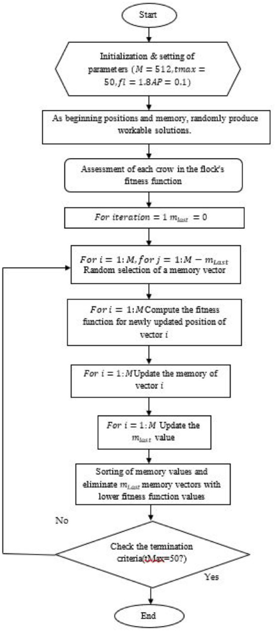
Proposed Ameliorate crow forage algorithm.
| (18) |
| (19) |
Here, the th number in the achieved sequence is denoted as and designates the control parameter where p is the chaotic sequence index. Initial point ( ) and value of are assumed to be 4 and 0.7, respectively. These parameters were selected to achieve better performance based on the experimentation. Because sine and logistic maps have greater statistical and dynamic features, this considerably increases the algorithm’s consistency and convergence rate. So, by combining chaotic map functions with a control operator, the optimization is enhanced. As a result, the suggested ICS and ELM algorithm, also known as the Ameliorate crow forage-ELM algorithm, will significantly enhance the classification performance. The most iterations possible, , is regarded as the optimization process’s halting criterion.
Result and Discussion
In visualizing the performances when we migrated from the on-premises platform to the cloud environment, the results from the standalone and cloud environments were combined. The Wisconsin Breast Cancer Diagnosis (WBCD) dataset was used in the investigation. The diagnosis property indicated whether the 569 entries in the dataset were malignant or benign.
Evaluation metrics
Five metrics are used in the quantitative analysis. Most of them fall into 1 of 3 groups. The position error is the first and is determined using the Euclidean distance P between the tumor target’s true position and the reconstruction findings’ location of the maximum energy region A small value is typically anticipatory, and the guiding idea is as follows:
| (20) |
Another confocal image noise measurement technique uses the signal to mean ratio (SMR), which is determined as follows:
| (21) |
where stands for the highest resolution of the recovered image. The greatest value outside of 50% attenuation range serves as the definition of . The Iaverage denotes the overall image’s average intensity. In general, improved imaging with less jitter and noise artifact suppression are associated with larger 2 criteria.
The last kind evaluates methods at the signal level using roughness (R) and coefficient of variation (CV). The measurements are fairly low, and the tumor response should, in theory, only be dispersed among a few sampling sites. If the 2 measurements are prominent, the signals will include meaningless responses. The signals are only utilized to quantitatively compare the performances of various approaches under the same experimental conditions because the properties of the signals vary across studies. The following equations are used in R and use the averaging method as the baseline:
| (22) |
| (23) |
where the letters and stand for each signal’s standard deviation and mean value, respectively. In general, the latter is very significant, while the first 2 values are all very small. Consequently, a CV might clearly show the differences between various approaches. This statistic is averaged over all channel signals to provide the result. In the numerator and denominator, for the SWVD, TSR, and averaging methods, respectively, represent the difference between 2 adjacent sample sites.
Our method makes use of the following computation techniques to categorize,
| (24) |
| (25) |
| (26) |
| (27) |
| (28) |
The number of positive cases in this instance that are considered positive is known as the TP (true positive). The numbers for true negatives, false negatives, and false positives are denoted by TN, FN, and FP, respectively. Recall has additional therapeutic value because it shows the proportion of samples that were declared positive. Macro-F, commonly referred to as macro-averaging, is a method for evaluating the effectiveness of numerous categories on a worldwide scale. It is calculated by averaging these per-category values after first calculating the F-scores for the n categories. A unique contingency table that enables performance visualization is the confusion matrix.
Seven distinct clusters are formed from the smaller patches that were selected from histology images in 4 different categories. Then, using ResNet50-128, the top 4 clusters with the average classification accuracy are selected. Table 3 displays the results and includes 25 201 128 × 128 pixel selected patches.
Table 3.
Lists how many patches of 512 × 512, and 128 × 128 pixels were taken from the training set’s breast images.
| Clusters | Normal | Benign | In situ | Invasive |
|---|---|---|---|---|
| 0 | 3050 | 2997 | 805 | 2017 |
| 1 | 771 | 2235 | 3044 | 1838 |
| 2 | 722 | 1700 | 2649 | 1986 |
| 3 | 2541 | 800 | 1225 | 1069 |
| 4 | 1113 | 885 | 596 | 513 |
| Selected | 4378 | 5584 | 4445 | 5839 |
Maximum performance in terms of accuracy (98.45%), precision (96%), recall (94%), and F1 score (95%) are offered by the Ameliorate Crow Forage-ELM Classifier. This merely improves these classifiers’ overall classification performance.
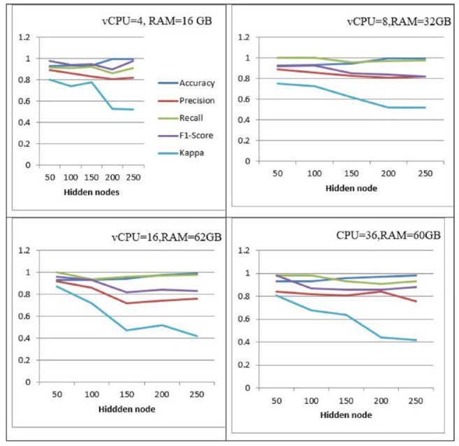
It can be shown that ELM performs better with 4 vCPUs and 16 GB of RAM than it does with 8 vCPUs and 32 GB of RAM whenever the specified is 200. The speed rises, though, and ELM achieves the best accuracy of 0.9868 when the virtual CPUs are set to 36 when the hidden layer nodes are set to 250, the virtual CPUs to 16, and the RAM to 64 GB. As can be seen, classification accuracy improves as more hidden layer nodes, virtual CPUs, and memory are added. With 250 hidden layer nodes, 36, vCPUs, and 60 GB of RAM, The most accurate classification is provided by ELM of 0.9868 depending on a number of parameters, as shown by the comparison above. Because of this, it is believed that the 250 hidden layer node ELM model, put into practice on a virtual machine with 36 vCPUs and 60 GB of RAM, is the most effective in classifying breast cancer.
Breast cancer is one of the leading causes of death among women. Although the chances of survival are improved by early discovery of this cancer, women who live in places with poor access to medical care do not have that option. Building disease prediction systems using machine learning and cloud computing technologies is of interest to many researchers. Cloud computing made Platform-as-a-Service (PaaS) accessible so that users could access resources as needed.
Conclusions
This research, an Extreme Learning Machine (ELM)-based architecture for cloud-based breast cancer diagnostics was suggested. Because the healthcare sector may use the system at any time, cloud computing benefits the industry. It can offer continuous services everywhere and at any time. Additionally, the cloud environment offers resources that raise the suggested model’s total classification accuracy. This method consists of modified 2-stage filtering, Savitzky-Golay (S-G) adaptive smoothing, and adaptive temporal window division. Several studies use the coefficient of variation (CV), roughness (R), positioning error (P), signal to max ratio (SMXR), and signal to mean ratio to compare it to the averaging and TSR approaches (SMR). We extract 2 different types of patches from the histology photographs, each having 512 pixels × 512 pixels and 128 pixels × 128 pixels with varied levels of feature density. They create a technique to instantly screen more racist and discriminatory patch of 128 × 128 pixel utilizing a range of machine learning algorithms including CNN. Patch features are extracted using ResNet50 as a feature extractor, while picture features are extracted using P-norm pooling. Based on the outcomes on the cloud-based ELM methodology outperforms older techniques on the Wisconsin Diagnostic Breast Cancer (WBCD) dataset.
By utilizing more resources in a cloud setting in the future, this framework can be expanded even further, perhaps improving categorization accuracy. The suggested paradigm will be used in the field of image processing, which supports a variety of applications such detection and recognition, diagnostic imaging, satellite images, and image enhancements. The performance of the provided framework can also be enhanced by adjusting a number of ELM parameters. The evaluation of the simulation model’s performance is shown in Table 1. While the quantity of 2 different types of patches that were taken from the training image collection is depicted in Table 2. Figure 5 shows the Graphical representation of the cloud computing environment. Also, the Performance of Ameliorate crow forage-ELM classifier is contained in Table 4.
Table 1.
Evaluation of the simulation model’s performance.
| Method | CV | R | Estimated positon (mm) | SMXR (dB) | SMR (dB) |
|---|---|---|---|---|---|
| Ave | 1263.80 | 1.00 | (47,46,39.4) | 1.76 | 21.84 |
| TSR | 739.52 | .69 | (47,50,37.6) | 2.33 | 24.33 |
| SWVD | 54.12 | .63 | (47,50,37.6) | 5.16 | 28.89 |
Table 2.
The quantity of 2 different types of patches that were taken from the training image collection.
| Class | Training set | 512 × 512 pixels | 128 × 128 pixels |
|---|---|---|---|
| Class | Training set | 512 × 512 pixels | 128 × 128 pixels |
| Normal | 54 | 1926 | 10 559 |
| Benign | 68 | 2414 | 13 249 |
| In situ | 62 | 2206 | 12 097 |
| Invasive | 61 | 2171 | 11 903 |
Figure 5.
Graphical representation of the cloud computing environment.
Table 4.
Performance of Ameliorate crow forage-ELM classifier.
| Output class | Number of inputs | Number of classified outputs | Accuracy(%) | Precision(%) | Recall(%) | F1 score(%) |
|---|---|---|---|---|---|---|
| Normal | 207 | 206 | 99.07 | 100 | 99 | 99 |
| Benign | 64 | 66 | 98.76 | 95 | 98 | 97 |
| Malignent | 51 | 50 | 98.45 | 96 | 94 | 95 |
Acknowledgments
We extend our heartfelt thanks to our institution for their support, as well as to our colleagues and mentors for their invaluable guidance and feedback throughout this research.
Footnotes
Funding: The author(s) received no financial support for the research, authorship, and/or publication of this article.
The author(s) declared no potential conflicts of interest with respect to the research, authorship, and/or publication of this article.
Author Contributions: Siva Shankar G led the conceptualization, methodology, and writing of the manuscript. Venkataramaiah Gude contributed to data analysis and algorithm development. Balasubramanian Prabhu Kavin provided substantial input on the deep learning models and virtualization techniques. Edeh Michael Onyema was responsible for experimental validation and interpretation of results. B.V.V. Siva Prasad supported the overall research design and manuscript revision. All authors reviewed and approved the final manuscript.
ORCID iD: Balasubramanian Prabhu Kavin  https://orcid.org/0000-0001-6939-4683
References
- 1. Vulli A, Srinivasu PN, Sashank MSK, et al. Fine-tuned DenseNet-169 for breast cancer metastasis prediction using FastAI and 1-cycle policy. Sensors. 2022;22:2988. [DOI] [PMC free article] [PubMed] [Google Scholar]
- 2. Chaurasia V, Pal S. Applications of machine learning techniques to predict diagnostic breast cancer. SN Comput. Sci. 2020;1:270. [Google Scholar]
- 3. Aroef C, Rivan Y, Rustam Z. Comparing random forest and support vector machines for breast cancer classification. Telkomnika. 2020;18:815-821. [Google Scholar]
- 4. Waqas K, Lima Ferreira J, Tsourdi E, et al. Updated guidance on the management of cancer treatment-induced bone loss (CTIBL) in pre- and postmenopausal women with early-stage breast cancer. J Bone Oncol. 2021;28:100355. [DOI] [PMC free article] [PubMed] [Google Scholar]
- 5. Anderson AS, Martin RM, Renehan AG, et al. ; UK NIHR Cancer and Nutrition Collaboration (Population Health Stream). Cancer survivorship, excess body fatness and weight-loss intervention-where are we in 2020? Br J Cancer. 2021;124:1057-1065. [DOI] [PMC free article] [PubMed] [Google Scholar]
- 6. Huang M, O’Shaughnessy J, Zhao J, et al. Association of Pathologic Complete Response with long-term survival outcomes in Triple-negative breast cancer: A meta-analysis. Cancer Res. 2020;80:5427-5434. [DOI] [PubMed] [Google Scholar]
- 7. Klement RJ, Champ CE, Kämmerer U, et al. Impact of a ketogenic diet intervention during radiotherapy on body composition: III-final results of the KETOCOMP study for breast cancer patients. Breast Cancer Res. 2020;22:94. [DOI] [PMC free article] [PubMed] [Google Scholar]
- 8. Patel S, Webster T, Baltodano P, Roth S. Search Strategies for a Systematic Review of Tamoxifen, Breast Reconstruction and Surgical Flap. Temple University Health Sciences, Philadelphia, USA; 2021. [Google Scholar]
- 9. Kiecolt-Glaser JK, Renna M, Peng J, et al. Breast cancer survivors’ typhoid vaccine responses: chemotherapy, obesity, and fitness make a difference. Brain Behav Immun. 2022;103:1-9. [DOI] [PMC free article] [PubMed] [Google Scholar]
- 10. O’Grady N, Gibbs DL, Abdilleh K, et al. PRoBE the cloud toolkit: Finding the best biomarkers of drug response within a breast cancer clinical trial. JAMIA Open. 2021;4. [DOI] [PMC free article] [PubMed] [Google Scholar]
- 11. Diaz O, Kushibar K, Osuala R, et al. Data preparation for artificial intelligence in medical imaging: A comprehensive guide to open-access platforms and tools. Phys Med. 2021;83:25-37. [DOI] [PubMed] [Google Scholar]
- 12. Shukla SK, Kumar BM, Sinha D, et al. Apprehending the effect of Internet of Things (IoT) enables big data processing through multinetwork in supporting high-quality food products to reduce breast cancer. J Food Qual. 2022;2022:1-12. [Google Scholar]
- 13. Aceto G, Persico V, Pescapé A. Industry 4.0 and health: Internet of things, big data, and cloud computing for healthcare 4.0. J Ind Inf Integr. 2020;18:100129. [Google Scholar]
- 14. McGrowder DA, Miller FG, Vaz K, et al. The utilization and benefits of telehealth services by health care professionals managing breast cancer patients during the COVID-19 pandemic. Healthcare. 2021;9(10):1401. [DOI] [PMC free article] [PubMed] [Google Scholar]
- 15. Bizot A, Karimi M, Rassy E, et al. Multicenter evaluation of breast cancer patients’ satisfaction and experience with oncology telemedicine visits during the COVID-19 pandemic. Br J Cancer. 2021;125:1486-1493. [DOI] [PMC free article] [PubMed] [Google Scholar]
- 16. Abdar M, Zomorodi-Moghadam M, Zhou X, et al. A new nested ensemble technique for automated diagnosis of breast cancer. Pattern Recognit Lett. 2020;132:123-131. [Google Scholar]
- 17. Khamparia A, Bharati S, Podder P, et al. Diagnosis of breast cancer based on modern mammography using hybrid transfer learning. Multidimens Syst Signal Process. 2021;32:747-765. [DOI] [PMC free article] [PubMed] [Google Scholar]
- 18. Huang H, Feng X, Zhou S, et al. A new fruit fly optimization algorithm enhanced support vector machine for diagnosis of breast cancer based on high-level features. BMC Bioinformatics. 2019;20:1-14. [DOI] [PMC free article] [PubMed] [Google Scholar]
- 19. Omondiagbe DA, Veeramani S, Sidhu AS. Machine learning classification techniques for breast cancer diagnosis. IOP Conf Ser Mater Sci Eng. 2019;495:012033. [Google Scholar]
- 20. Kassani SH, Kassani PH, Wesolowski MJ, Schneider KA, Deters R. Breast cancer diagnosis with transfer learning and global pooling. In: Int. Conf. ICT Converg. 2019, 519-524. Jeju Island, South Korea: IEEE. [Google Scholar]
- 21. Bourouis S, Band S, Mosavi A, et al. Meta-heuristic algorithm-tuned neural network for breast cancer diagnosis using ultrasound images. Front Oncol. 2022;12:834028. [DOI] [PMC free article] [PubMed] [Google Scholar]
- 22. Jang JY, Kim YS, Kang KN, et al. Multiple microRNAs as biomarkers for early breast cancer diagnosis. Mol Clin Oncol. 2021;14:31-1. [DOI] [PMC free article] [PubMed] [Google Scholar]
- 23. Wang S, Wang Y, Wang D, et al. An improved random forest-based rule extraction method for breast cancer diagnosis. Appl Soft Comput. 2020;86:105941. [Google Scholar]
- 24. Desai M, Shah M. An anatomization on breast cancer detection and diagnosis employing multi-layer perceptron neural network (MLP) and convolutional neural network (CNN). Clin eHealth. 2021;4:1-11. [Google Scholar]
- 25. Khan S, Islam N, Jan Z, Ud Din I, Rodrigues JJPC. A novel deep learning based framework for the detection and classification of breast cancer using transfer learning. Pattern Recognit Lett. 2019;125:1-6. [Google Scholar]
- 26. Nwosu OF. Cloud-Enhanced Machine Learning for Handwritten Character Recognition in Dementia Patients. In Driving Transformative Technology Trends With Cloud Computing, Chap 17. 2024;1-14. [Google Scholar]
- 27. Mohit T, Tripti T, Manal K, Anit NR, et al. Detection of coronavirus disease in human body using convolutional neural network. International Journal of Advanced Science and Technology. 2020;29:2861-2866. [Google Scholar]
- 28. Kaur A, Kaushal C, Sandhu JK, et al. Histopathological image diagnosis for breast cancer diagnosis based on deep mutual learning. Diagnostics. 2023;14:95. [DOI] [PMC free article] [PubMed] [Google Scholar]