Insights from qualitative and bifurcation analysis of COVID-19 vaccination model in Bangladesh

Abstract

The unprecedented global impact of the 2019 coronavirus disease (COVID-19) has necessitated a comprehensive understanding of its transmission dynamics and control measures. In this study, we present a detailed analysis of a COVID-19 vaccination model tailored to the context of Bangladesh, incorporating dual-dose vaccination strategies. By employing qualitative and bifurcation analysis techniques, we investigate the equilibrium points, effective reproduction number (R0), and critical thresholds that influence the prevalence and control of COVID-19 in the region. Our findings reveal insights into the effectiveness of vaccination programs and provide a framework for developing targeted control plans. Through a rigorous examination of model parameters and sensitivity analysis, we identify key factors driving COVID-19 transmission dynamics, emphasizing the significance of vaccination rates and other critical parameters. The validation of our model against real-world data underscores its utility in informing evidence-based decision-making for managing the COVID-19 pandemic in Bangladesh and beyond.

Introduction

Certainly, many people suffer from several infectious diseases, including tuberculosis, measles, influenza, HIV, severe acute respiratory syndrome (SARs) and malaria, and a large number of those infected patients die around the world every year. Infectious diseases are also transmissible or communicable diseases caused by various pathogens, bacteria, fungi, and viruses [1]. Even though the communicable disease-related mortality rate is gradually decreasing worldwide, it is still relatively high in poor and developing countries due to a lack of awareness, poor prevention, and inappropriate infection-controlling systems [2]. However, in the last decade, infectious diseases, such as plague, AIDS, severe acute respiratory syndrome (SARS) virus, and bird flu, emerged, and the world had to face huge challenges in controlling these diseases [3]. From the end of 2019 until now, the world has again faced a significant challenge again due to the new coronavirus (COVID-19). The coronavirus (COVID-19) first emerged in Wuhan city of Hubei province of China at the end of December 2019. Subsequently, it was identified in most of the countries in the world, with more than 770 million persons infected as of 24 September 2023 [4, 5]. It is a highly contagious disease that spreads from person to person through coughing or sneezing [6]. A COVID-19-infected person may suffer symptoms like fever, dry cough, flu, tiredness, diarrhea, sore throat, body aches, and shortness of breath [7]. The appearance of these symptoms in a person infected with COVID-19 usually takes two to fourteen days, and this long-term exposure or latent period makes this disease exceptional compared to other infectious diseases [8]. Also, people with strong immunity are mildly affected by this disease and do not need advanced treatment. But people suffering from other serious diseases, including asthma, heart disease, and diabetes, are particularly vulnerable to severe outcomes from COVID-19. These individuals are at higher risk of experiencing complications that can lead to severe illness or even death if they contract the virus [9].

To prevent the spread of the COVID-19 outbreak, the government has taken some essential steps such as local or area-based lockdown, the shutdown of all government and private organizations, diagnosis of the suspected cases, home quarantine and COVID-19 tests for suspected persons, isolation or hospitalization of infected persons, the establishment of some dedicated corona hospitals, increasing testing capacities, improving social awareness, enforcing social distancing, and launching vaccination [10].

Vaccination is a more effective way to prevent or control the spread of COVID-19. Although the COVID-19 vaccines produced by different medical agencies are now available in the world market, it was initially the most challenging task to invent a vaccine. Launching the first vaccine on the market took over one and a half years. At first, some vaccines were named Pfizer, AstraZeneca AZD1222, Moderna, and J&J Ad26.COV2.S got approval from the European and Italian medicine agencies on 13th March 2021 to be injected into the patient’s body [11]. Vaccination substantially prevents death from the virus infection and increases immunity in the human body against the virus. The vaccine efficacy was reported at about 94% for Moderna, 95% for Pfizer, 81.3% for AZD122, and 85% for J&J Ad26.COV2.S after vaccination [12–15]. The Strategic Advisory Group of Experts on Immunization (SAGE) suggests two doses of each vaccine for a complete series, with the interval between the vaccine doses being 21 days and 28 days for the Pfizer and Moderna vaccines, respectively; however, an extended time interval up to 42 days is also allowed for some cases [16].

On March 11, 2020, the World Health Organization (WHO), a global public health organization, declared COVID-19 as a global pandemic [17]. Based on Woldometer data up to July 20, 2021, 191.7 million people were infected in 213 countries around the world, with more than 4,113,054 deaths and 174.5 million recoveries [18]. The highest number of infected people, about 35 million, were reported in the USA [19]. The infection rate was increasing rapidly in some European countries, including Italy, France, England, Spain, Russia, and Germany, as well as in Asian countries, such as India [18].

In contrast, the flow of infections was shallow at the beginning of the epidemic. However, later, both infection and death rates increased dramatically in Bangladesh. The first case was detected on 8th March 2020 by the Institute of Epidemiology, Disease Control and Research (IEDCR) [20]. As per the Woldometer record, up to 13th April 2024, a total of 2.05 million infected cases have been officially identified, with 29,493 deaths and more than 2.02 million recovered [21].

To control and prevent the spread of COVID-19, Bangladesh implemented several key initiatives, including lockdowns and movement restrictions, mass vaccination campaign, public awareness, expansion of testing facilities, quarantine and isolation measures, international collaboration and aid. Despite these key initiatives, controlling and preventing the COVID-19 pandemic is becoming more challenging for Bangladesh due to its high population, limited testing facilities, poor healthcare systems, and other limitations. However, an appropriate vaccination strategy plan is expected to be more effective in preventing the spread of COVID-19. Bangladesh began its COVID-19 vaccination campaign on January 27, 2021. The campaign initially prioritized frontline workers, including healthcare professionals, police, and military personnel, as well as elderly citizens and those with pre-existing conditions. The country rolled out the vaccine nationwide after receiving its first shipments of the Oxford-AstraZeneca vaccine, produced by the Serum Institute of India [22].

Many researchers from different fields are continuously working to understand the behavior of COVID-19. In particular, numerous mathematical models have been developed to predict the spread of infectious diseases and inform strategies for controlling outbreaks in specific regions [23–30]. The Susceptible-Infected Recovery (SIR) mathematical model commonly used for various epidemics was first developed in 1927 by the famous epidemiologists Kermack and Mackendrick [31]. Zhang et al. studied COVID-19 infection on the Diamond Princess cruise ship, estimated the reproduction number of a novel coronavirus in the early stage of the outbreak, and made a prediction of daily new cases on the ship [32]. A nonlinear mathematical model was studied to understand and analyze the transmission dynamics of the COVID-19 outbreak by Riyapan et al. [33]. In order to investigate the scenarios of different levels of vaccine efficacy and explore the diseased dynamics of COVID-19, a mathematical model considering heterogeneous populations was proposed [33]. To evaluate the effectiveness of COVID-19 vaccination programs, Watson et al., 2022 estimated the number of additional lives that would have been lost if vaccines had not been distributed [34]. In [35], the authors studied a mathematical modeling approach to identify the critical factors of a vaccination program. The Partial Rank Correlation Coefficient (PRCC) technique and sensitivity analysis are conducted to pinpoint the most significant model parameters that affect transmission and disease prevalence [36]. A mathematical model is proposed to explore the potential outcomes of COVID-19 vaccination and the effects of various factors, such as vaccine type, age group eligibility, vaccination strategy, and population coverage [37]. Additionally, numerous studies have been conducted to clarify COVID-19 transmission dynamics [38–44].

Although the COVID-19 double-dose vaccination SEIR model is common in literature [45–47], we used a modified version of the SEIR model with double-dose vaccination in our study, which is a novel contribution to explore the dynamics of COVID-19 in the Bangladesh setting, as far to our knowledge. Here, we distinguished the infected population into two additional compartments: Mild (M) and Critical (C). We considered Mild (M) individuals who are infected, infectious and have mild respiratory illness symptoms such as nasal congestion, runny nose, and a sore throat. Critical (C) individuals who are infected, infectious and have severe symptoms including shortness of breath, chest discomfort and bluish face. We also incorporated first and second-dose vaccines to explore the impact of vaccination and other control strategies for reducing the burden of COVID-19 in Bangladesh. Here, we allow first- and second-dose vaccinated people to move to the latent compartment due to the loss of immunity, which was not considered in the previous modelling studies [45, 48, 49].

In the current study, we developed a modified nonlinear mathematical model (seven compartments) with double-dose vaccination in Bangladesh. Here, we performed a rigorous analysis of the system properties and solutions to predict both the early and late-time behaviour of the model. After deriving the effective reproduction number (R0) for COVID-19 using the next-generation matrix technique, we investigate the impact of relative magnitudes on the infected populations in Bangladesh. COVID-19 can spread in Bangladesh’s population only if R0>1 (epidemic) but can maintained in a population without the need for external inputs when R0 < 1. A disease-free population will result when effective reproduction number R0<1, which means the disease naturally dies out. Furthermore, if R0>1, then the COVID-19 virus persist in the Bangladesh population. Therefore, in order to control transmission, the period of infectiousness needs to be reduced until R0<1. We completed a bifurcation analysis to identify critical points where small changes in a parameter can lead to substantial shifts in the system’s behavior.

Next, we estimate the parameters to enhance the model’s predictive capabilities. We also performed a sensitivity analysis of the model outcomes and parameters and found that the contact rate of COVID-19 had the largest influence on disease prevalence and explored the impact of different interventions, including vaccination strategy, on the dynamics of the infected population in Bangladesh. In conclusion, our research findings will provide a better understanding of the changing epidemiology of COVID-19 in terms of vaccination coverage and will support future policy and planning of the disease control efforts in Bangladesh. In addition, our COVID-19 vaccination model provides insights with wide-ranging implications for global public health as the virus continues to impact populations worldwide. The model can be adapted to other settings with similar epidemiological conditions, and the analysis of the effective reproduction number (R₀) offers a universal understanding of transmission dynamics, supporting policymakers in their efforts to control the spread.

This study is designed as follows: A brief introduction is written in Introduction section. The mathematical formulation of the compartmental model is discussed in Materials and Methods section. The effective reproduction number, the existence of equilibriums, stability analysis, parameters estimation, sensitivity analysis, and numerical simulations are performed in Results section. Finally, a brief discussion and conclusion are outlined at the end of this study.

Materials and methods

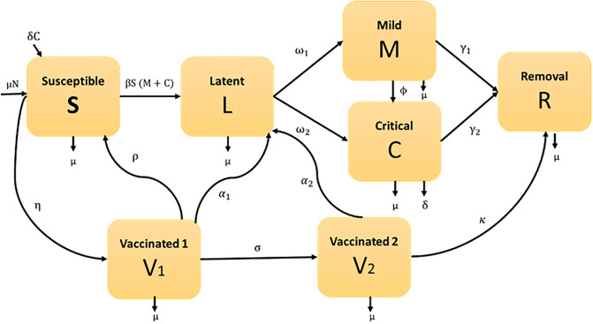
We developed a compartmental model to examine the transmission dynamics of COVID-19 with dual dose vaccinations, where the total population size is divided into seven separated compartments such as susceptible class (S), uninfected individuals who are susceptible to COVID-19 infection. The rate of change of the susceptible population decreases as individuals move from the susceptible compartment to the Latent and first dose vaccinated compartments, First dose vaccinated class (V₁), who received first dose vaccine and increases as susceptible individuals receive the first dose vaccine; Second dose vaccinated class (V₂), who received second dose vaccine and increases as first dose vaccinated individuals receive the second dose vaccine; Latent class (L), those who are infected but not infectious. The latent individuals move from the susceptible compartment at a rate dependent on the transmission rate and the current number of mild and critical individuals, Mild class (M), who are infected, infectious and have mild respiratory illness symptoms such as nasal congestion, runny nose, and a sore throat. A proportion of the latent individuals develop mild symptoms and move into the Mild compartment, Critical class (C), who are infected, infectious and have severe symptoms including shortness of breath, chest discomfort, and bluish face. A proportion of the latent individuals develop critical symptoms and move into the critical compartment. The difference between Mild and Critical individuals is particularly useful in scenarios where Mild cases may be underreported or where public health interventions differ for mild versus critical cases (e.g., hospitalization for critical cases versus home isolation for mild cases). It also helps policymakers allocate resources effectively and predict the outcomes of different intervention strategies; and recovered class (R), those who are neither infectious nor susceptible, including people in treatment, isolation, no longer mixing/contacting others (e.g. no longer injecting drugs) or dead. The recovery population increases as mild, critical and second-dose vaccinated individuals recover from the disease. Assume the size of the total population at any time t is N(t), which is constant (that means the only way a person can leave the susceptible group is to be vaccinated or infected, and the only way a person can leave vaccinated or infected group is to recover due to received immunity), age, sex, race and social status do not affect the probability of being infected, and homogeneously mixed, and it can be written as:

$$\mathrm{N}\left(\mathrm{t}\right)=\mathrm{S}\left(\mathrm{t}\right)+{\mathrm{V}}_1\left(\mathrm{t}\right)+{\mathrm{V}}_2\left(\mathrm{t}\right)+\mathrm{L}\left(\mathrm{t}\right)+\mathrm{M}\left(\mathrm{t}\right)+\mathrm{C}\left(\mathrm{t}\right)+\mathrm{R}\left(\mathrm{t}\right).$$ (1)

Consider all deaths replaced as newborns in the susceptible compartment for keeping the population size constant. The parameter η is the rate of getting the first dose of vaccine. First-dosed vaccinated individuals V₁ move to the susceptible group at a rate ρ due to the rate of loss of immunity and the rest of the individuals move to the second-dosed vaccinated individuals V₂ at a rate σ. The first-dose and second-dose vaccinated persons who lose immunity are infected again and move to the Latent class with the rate of α₁ and α₂, respectively. The second-dosed vaccinated individual also moves to the recovery compartment at a rate κ. The following parameters are also used: ω₁, ω₂ denote the rates at which the latent population becomes infectious Mildly and Critically respectively; γ₁, γ₂ represent the rates at which the Mildly and Critically infected individuals are recovered due to treatment respectively; β is the contact rate between Mild or Critical class and susceptible individual; ϕ is the transfer rate of Mildly infected individuals to Critically infected individuals due to co-infection with other diseases; μ represents the birth or death rate due to natural causes which occur in all states; and δ denotes the per capita constant rate of COVID-19 related deaths. The compartmental elucidation of the model is presented in Fig 1.

Fig 1. Graphic illustration of COVID-19 model in Bangladesh.

English letters in boxes designate state variables (model compartments), while Greek letters represent model parameters.

From the compartmental representation of the model (Fig 1), the transmission mechanism of COVID-19 can be written by the following system of differential equations:

$$\frac{\mathrm{d}\mathrm{S}}{\mathrm{d}\mathrm{t}}=\mathrm{\mu }\mathrm{N}+\mathrm{\rho }{\mathrm{V}}_1+\delta \mathrm{C}-\beta \mathrm{S}\left(\mathrm{M}+\mathrm{C}\right)-\mathrm{\eta }\mathrm{S}-\mathrm{\mu }\mathrm{S},$$ (2)

$$\frac{\mathrm{d}{\mathrm{V}}_1}{\mathrm{d}\mathrm{t}}=\mathrm{\eta }\mathrm{S}-\left(\mathrm{\rho }+\mathrm{\sigma }+{\mathrm{\alpha }}_1+\mathrm{\mu }\right){\mathrm{V}}_1,$$ (3)

$$\frac{\mathrm{d}{\mathrm{V}}_2}{\mathrm{d}\mathrm{t}}=\mathrm{\sigma }{\mathrm{V}}_1-\left(\mathrm{\kappa }+{\mathrm{\alpha }}_2+\mathrm{\mu }\right){\mathrm{V}}_2,$$ (4)

$$\frac{\mathrm{d}\mathrm{L}}{\mathrm{d}\mathrm{t}}=\beta \mathrm{S}\left(\mathrm{M}+\mathrm{C}\right)+{\mathrm{\alpha }}_1{\mathrm{V}}_1+{\mathrm{\alpha }}_2{\mathrm{V}}_2-\left({\mathrm{\omega }}_1+{\mathrm{\omega }}_2+\mathrm{\mu }\right)\mathrm{L},$$ (5)

$$\frac{\mathrm{d}\mathrm{M}}{\mathrm{d}\mathrm{t}}={\mathrm{\omega }}_1\mathrm{L}-\left(\varphi +{\mathrm{\gamma }}_1+\mathrm{\mu }\right)\mathrm{M},$$ (6)

$$\frac{\mathrm{d}\mathrm{C}}{\mathrm{d}\mathrm{t}}={\mathrm{\omega }}_2\mathrm{L}+\varphi \mathrm{M}-\left({\mathrm{\gamma }}_2+\delta +\mathrm{\mu }\right)\mathrm{C},$$ (7)

$$\frac{\mathrm{d}\mathrm{R}}{\mathrm{d}\mathrm{t}}={\mathrm{\gamma }}_1\mathrm{M}+{\mathrm{\gamma }}_2\mathrm{C}+\mathrm{\kappa }{\mathrm{V}}_2-\mathrm{\mu }\mathrm{R}.$$ (8)

The above system’s (2)-(8) initial conditions are as follows:

$$\mathrm{S}\left(0\right)\ge 0,{\mathrm{V}}_1\left(0\right)\ge 0,{\mathrm{V}}_2\left(0\right)\ge 0,\mathrm{L}\left(0\right)\ge 0,\mathrm{M}\left(0\right)\ge 0,\mathrm{C}\left(0\right)\ge 0,\mathrm{R}\left(0\right)\ge 0.$$ (9)

The existence and the non-negativity of the solutions of (2)-(8) and the initial conditions (9) can easily be shown for all t ≥ 0.

By summing Eqs (2)–(8), we have:

$$\frac{\mathrm{d}\mathrm{N}}{\mathrm{d}\mathrm{t}}=\frac{\mathrm{d}\mathrm{S}}{\mathrm{d}\mathrm{t}}+\frac{\mathrm{d}{\mathrm{V}}_1}{\mathrm{d}\mathrm{t}}+\frac{\mathrm{d}{\mathrm{V}}_2}{\mathrm{d}\mathrm{t}}+\frac{\mathrm{d}\mathrm{L}}{\mathrm{d}\mathrm{t}}+\frac{\mathrm{d}\mathrm{M}}{\mathrm{d}\mathrm{t}}+\frac{\mathrm{d}\mathrm{C}}{\mathrm{d}\mathrm{t}}+\frac{\mathrm{d}\mathrm{R}}{\mathrm{d}\mathrm{t}}=0.$$

Integrating this equation, we get

$$\mathrm{N}\left(\mathrm{t}\right)=\mathrm{C}\mathrm{o}\mathrm{n}\mathrm{s}\mathrm{t}\mathrm{a}\mathrm{n}\mathrm{t}.$$

The fixed population size and positivity of solutions clearly indicate the boundedness of individually of the states S, V₁, V₂, L, M, C, R.

In the model (2)—(8), the recovered individuals R(t) does not present in the Eqs (2)–(7) i.e., these equations are free of R(t). Hence, to track the trajectory of disease incidence and prevalence, we can give our effort into the below-reduced system

$$\frac{\mathrm{d}\mathrm{S}}{\mathrm{d}\mathrm{t}}=\mathrm{\mu }\mathrm{N}+\mathrm{\rho }{\mathrm{V}}_1+\delta \mathrm{C}-\beta \mathrm{S}\left(\mathrm{M}+\mathrm{C}\right)-\mathrm{\eta }\mathrm{S}-\mathrm{\mu }\mathrm{S},$$ (10)

$$\frac{\mathrm{d}{\mathrm{V}}_1}{\mathrm{d}\mathrm{t}}=\mathrm{\eta }\mathrm{S}-\left(\mathrm{\rho }+\mathrm{\sigma }+{\mathrm{\alpha }}_1+\mathrm{\mu }\right){\mathrm{V}}_1,$$ (11)

$$\frac{\mathrm{d}{\mathrm{V}}_2}{\mathrm{d}\mathrm{t}}=\mathrm{\sigma }{\mathrm{V}}_1-\left(\mathrm{\kappa }+{\mathrm{\alpha }}_2+\mathrm{\mu }\right){\mathrm{V}}_2,$$ (12)

$$\frac{\mathrm{d}\mathrm{L}}{\mathrm{d}\mathrm{t}}=\beta \mathrm{S}\left(\mathrm{M}+\mathrm{C}\right)+{\mathrm{\alpha }}_1{\mathrm{V}}_1+{\mathrm{\alpha }}_2{\mathrm{V}}_2-\left({\mathrm{\omega }}_1+{\mathrm{\omega }}_2+\mathrm{\mu }\right)\mathrm{L},$$ (13)

$$\frac{\mathrm{d}\mathrm{M}}{\mathrm{d}\mathrm{t}}={\mathrm{\omega }}_1\mathrm{L}-\left(\varphi +{\mathrm{\gamma }}_1+\mathrm{\mu }\right)\mathrm{M},$$ (14)

$$\frac{\mathrm{d}\mathrm{C}}{\mathrm{d}\mathrm{t}}={\mathrm{\omega }}_2\mathrm{L}+\varphi \mathrm{M}-\left({\mathrm{\gamma }}_2+\delta +\mathrm{\mu }\right)\mathrm{C},$$ (15)

Since the solutions of this system are non-negative and bounded the feasible solutions set for Eqs (10)–(15) enter the region:

$$\mathrm{D}=\left\{\left(\mathrm{S},{\mathrm{V}}_1,{\mathrm{V}}_2,\mathrm{L},\mathrm{M},\mathrm{C},\right)\in {\mathrm{R}}_{+}^6:\mathrm{S}+{\mathrm{V}}_1+{\mathrm{V}}_2+\mathrm{L}+\mathrm{M}+\mathrm{C}=\mathrm{N}\right\}.$$ (16)

For the system (10)–(15), D is the positively invariant region. Consequently, we consider system (10)–(15) in the set D.

Ethical approval

This study is based on aggregated monthly surveillance data from the COVID-19 dynamic dashboard provided by the Bangladesh Demographic and Health Survey. No confidential information was included because mathematical analyses were performed at the aggregate level. Data have no names and date of birth, so re-identification will not be possible. We believe that these data are truly de-identified and that the information listed in the line can’t be able to be attributed to individuals. We compiled data from the publicly available website https://dashboard.dghs.gov.bd/pages/covid19-bedstatus-display-graph.php. Therefore, no ethical approval is required.

Results

Effective reproduction number

The effective reproduction number, R₀, is a key concept in epidemiology that represents the average number of secondary infections generated by a single infected individual in a fully susceptible population. It is a critical measure for understanding the potential spread of an infectious disease. If R₀ > 1, the disease is likely to spread into the community and potentially cause an epidemic; if R₀ < 1, the infection will eventually die out. R₀ is crucial for predicting the duration and size of an epidemic and helps determine the level of intervention needed to control the spread. It also allows for the estimation of the herd immunity threshold, which is the proportion of the population that must be immune to prevent further transmission and is directly related to R₀. In conclusion, R₀ is a vital parameter for forecasting whether a disease will persist or be eradicated in a population.

The effective reproduction number can be derived using the next-generation matrix method (which is effectively a table describing the number of new infections generated by each individual infected with a particular strain) [50, 51]. The next-generation matrix is the product of matrices F and −V⁻¹, where matrix F represents the transmission components of infected states and the matrix V describes transitions between, and out of the infected states. In this model, the infected compartments are L, M, and C. The matrices F and V for this model are given as

$$\mathrm{F}=\left(\begin{array}{ccc}0& \beta {\mathrm{S}}^0& \beta {\mathrm{S}}^0\\ 0& 0& 0\\ 0& 0& 0\end{array}\right)$$

and

$$\mathrm{V}=\left(\begin{array}{ccc}-({\mathrm{\omega }}_1+{\mathrm{\omega }}_2+\mathrm{\mu })& 0& 0\\ {\mathrm{\omega }}_1& -(\varphi +{\mathrm{\gamma }}_1+\mathrm{\mu })& 0\\ {\mathrm{\omega }}_2& \varphi & -({\mathrm{\gamma }}_2+\delta +\mathrm{\mu })\end{array}\right).$$

The next-generation matrix K is given by [51]

$$\begin{array}{l}\text{K}=\text{F}(-{\text{V}}^{-1})\\ =\left(\begin{array}{ccc}0& {\beta \text{S}}^0& {\beta \text{S}}^0\\ 0& 0& 0\\ 0& 0& 0\end{array}\right)\left(\begin{array}{ccc}\frac{1}{\left({\omega }_1+{\omega }_2+\mu \right)}& 0& 0\\ \frac{{\omega }_1}{\left({\omega }_1+{\omega }_2+\mu \right)\left(\varphi +{\gamma }_1+\mu \right)}& \frac{1}{\left(\varphi +{\gamma }_1+\mu \right)}& 0\\ \frac{{\omega }_1\varphi +{\omega }_2\left(\varphi +{\gamma }_1+\mu \right)}{\left({\omega }_1+{\omega }_2+\mu \right)\left(\varphi +{\gamma }_1+\mu \right)\left({\gamma }_2+\delta +\mu \right)}& \frac{\varphi }{\left({\gamma }_2+\delta +\mu \right)\left(\varphi +{\gamma }_1+\mu \right)}& \frac{1}{\left({\gamma }_2+\delta +\mu \right)}\end{array}\right)\\ =\left(\begin{array}{ccc}\frac{{\beta \text{S}}^0\left[{\omega }_1\left(\varphi +{\gamma }_2+\delta +\mu \right)+{\omega }_2\left(\varphi +{\gamma }_1+\mu \right)\right]}{\left({\omega }_1+{\omega }_2+\mu \right)\left(\varphi +{\gamma }_1+\mu \right)\left({\gamma }_2+\delta +\mu \right)}& \frac{{\beta \text{S}}^0\left[\left(\varphi +{\gamma }_2+\delta +\mu \right)\right]}{\left(\varphi +{\gamma }_1+\mu \right)\left({\gamma }_2+\delta +\mu \right)}& \frac{{\beta \text{S}}^0}{\left({\gamma }_2+\delta +\mu \right)}\\ 0& 0& 0\\ 0& 0& 0\end{array}\right).\end{array}$$

The spectral radius of the next generation matrix K is considered the effective reproduction number. Hence the effective reproduction number is obtained as:

$$\begin{array}{ll}{\text{R}}_0\hfill & \frac{{\beta \text{S}}^0\left[{\omega }_1\left(\varphi +{\gamma }_2+\delta +\mu \right)+{\omega }_2\left(\varphi +{\gamma }_1+\mu \right)\right]}{\left({\omega }_1+{\omega }_2+\mu \right)\left(\varphi +{\gamma }_1+\mu \right)\left({\gamma }_2+\delta +\mu \right)},\hfill \\ \hfill & =\frac{\beta \mu \text{N}\left(\rho +\sigma +{\alpha }_1+\mu \right)\left[{\omega }_1\left(\varphi +{\gamma }_2+\delta +\mu \right)+{\omega }_2\left(\varphi +{\gamma }_1+\mu \right)\right]}{\left(\left(\rho +\sigma ++\mu \right)\left(\eta +\mu \right)-\eta \rho \right)\left({\omega }_1+{\omega }_2+\mu \right)\left(\varphi +{\gamma }_1+\mu \right)\left({\gamma }_2+\delta +\mu \right)}\hfill \end{array}.$$

Existence of equilibria

We found two equilibrium solutions: the disease-free equilibrium happens when R₀ is less than one i.e., R₀ < 1 and the disease endemic equilibrium happens when R₀ is greater than one i.e., R₀ > 1. We deliberate these in the following order.

Clearly, Eqs (10)–(15) always have an infection-free equilibrium

$${\mathrm{E}}^0=\left({\mathrm{S}}^0,{\mathrm{V}}_1^0,{\mathrm{V}}_2^0,{\mathrm{L}}^0,{\mathrm{M}}^0,{\mathrm{C}}^0\right),$$

where,

$${\mathrm{S}}^0=\frac{\mathrm{\mu }\mathrm{N}(\mathrm{\rho }+\mathrm{\sigma }+{\mathrm{\alpha }}_1+\mathrm{\mu })}{\left(\left(\mathrm{\rho }+\mathrm{\sigma }+{\mathrm{\alpha }}_1+\mathrm{\mu }\right)\left(\mathrm{\eta }+\mathrm{\mu }\right)-\mathrm{\eta }\mathrm{\rho }\right)},$$

$${\mathrm{V}}_1^0=\frac{\mathrm{\mu }\mathrm{\eta }\mathrm{N}}{\left(\left(\mathrm{\rho }+\mathrm{\sigma }+{\mathrm{\alpha }}_1+\mathrm{\mu }\right)\left(\mathrm{\eta }+\mathrm{\mu }\right)-\mathrm{\eta }\mathrm{\rho }\right)},$$

$${\mathrm{V}}_2^0=\frac{\mathrm{\mu }\mathrm{\eta }\mathrm{\sigma }\mathrm{N}}{\left(\left(\mathrm{\rho }+\mathrm{\sigma }+{\mathrm{\alpha }}_1+\mathrm{\mu }\right)\left(\mathrm{\eta }+\mathrm{\mu }\right)-\mathrm{\eta }\mathrm{\rho }\right)\left(\mathrm{\kappa }+{\mathrm{\alpha }}_2+\mathrm{\mu }\right)},$$

$${\mathrm{L}}^0=0,$$

$${\mathrm{M}}^0=0,$$

$${\mathrm{C}}^0=0.$$

From Eqs (10)–(15) we can also determine the endemic equilibrium

$${\mathrm{E}}^{*}=\left({\mathrm{S}}^{*},{\mathrm{V}}_1^{*},{\mathrm{V}}_2^{*},{\mathrm{L}}^{*},{\mathrm{M}}^{*},{\mathrm{C}}^{*}\right),$$

where

$${\mathrm{S}}^{*}=\frac{{\mathrm{S}}^0}{{\mathrm{R}}_0},$$

$$V_1^{*}=\frac{\mathrm{\eta }{\mathrm{S}}^0}{{\mathrm{R}}_0(\mathrm{\rho }+\mathrm{\sigma }+{\mathrm{\alpha }}_1+\mathrm{\mu })},$$

$$V_2^{*}=\frac{\mathrm{\sigma }\mathrm{\eta }{\mathrm{S}}^0}{{\mathrm{R}}_0(\mathrm{\rho }+\mathrm{\sigma }+{\mathrm{\alpha }}_1+\mathrm{\mu })\left(\mathrm{\kappa }+{\mathrm{\alpha }}_2+\mathrm{\mu }\right)},$$

$${\mathrm{L}}^{*}=\frac{\mathrm{\mu }\mathrm{N}\left({\mathrm{R}}_0-1\right)\left(\varphi +{\mathrm{\gamma }}_1+\mathrm{\mu }\right)\left(\delta +{\mathrm{\gamma }}_2+\mathrm{\mu }\right)}{{\mathrm{R}}_0\left[\left({\mathrm{\omega }}_1+{\mathrm{\omega }}_2+\mathrm{\mu }\right)\left(\varphi +{\mathrm{\gamma }}_1+\mathrm{\mu }\right)\left(\delta +{\mathrm{\gamma }}_2+\mathrm{\mu }\right)-\delta \left\{{\mathrm{\omega }}_2\left(\varphi +{\mathrm{\gamma }}_1+\mathrm{\mu }\right)+\varphi {\mathrm{\omega }}_1\right\}\right]},$$

$${\mathrm{M}}^{*}=\frac{\mathrm{\mu }\mathrm{N}{\mathrm{\omega }}_1\left({\mathrm{R}}_0-1\right)\left(\delta +{\mathrm{\gamma }}_2+\mathrm{\mu }\right)}{{\mathrm{R}}_0\left[\left({\mathrm{\omega }}_1+{\mathrm{\omega }}_2+\mathrm{\mu }\right)\left(\varphi +{\mathrm{\gamma }}_1+\mathrm{\mu }\right)\left(\delta +{\mathrm{\gamma }}_2+\mathrm{\mu }\right)-\delta \left\{{\mathrm{\omega }}_2\left(\varphi +{\mathrm{\gamma }}_1+\mathrm{\mu }\right)+\varphi {\mathrm{\omega }}_1\right\}\right]},$$

$${\mathrm{C}}^{*}=\frac{\mathrm{\mu }\mathrm{N}\left({\mathrm{R}}_0-1\right)\left({\mathrm{\omega }}_2\left(\varphi +{\mathrm{\gamma }}_1+\mathrm{\mu }\right)+\varphi {\mathrm{\omega }}_1\right)}{{\mathrm{R}}_0\left[\left({\mathrm{\omega }}_1+{\mathrm{\omega }}_2+\mathrm{\mu }\right)\left(\varphi +{\mathrm{\gamma }}_1+\mathrm{\mu }\right)\left(\delta +{\mathrm{\gamma }}_2+\mathrm{\mu }\right)-\delta \left\{{\mathrm{\omega }}_2\left(\varphi +{\mathrm{\gamma }}_1+\mathrm{\mu }\right)+\varphi {\mathrm{\omega }}_1\right\}\right]}.$$ (17)

From the Eq (17), the denominator of S*, $V_1^{*},V_2^{*}$ are positive as all of the included parameter’s values are positive, whereas the denominator L*, M*, and C* depends on

$$\begin{array}{l}\left[\left({\omega }_1+{\omega }_2+\mu \right)\left(\varphi +{\gamma }_1+\mu \right)\left(\delta +{\gamma }_2+\mu \right)-\delta \left\{{\omega }_2\left(\varphi +{\gamma }_1+\mu \right)+\varphi {\omega }_1\right\}\right]\\ \Rightarrow \left[\left(0.034+5.78\times {10}^{-4}+\frac{1}{70}\right)\left(0.3+0.02+\frac{1}{70}\right)\left(0.125+0.01+\frac{1}{70}\right)-0.125\left\{5.78\times {10}^{-4}\left(0.3+0.02+\frac{1}{70}\right)+0.3\times 0.034\right\}\right]=1.139\times {10}^{-3}>0\end{array}$$ (18)

Eq (18) shows that if we put the values of ω₁, ω₂, γ₁, γ₂, μ, δ, ϕ from Table 1, we get a positive value from this equation.Eq (17) displays that the endemic equilibrium point ${\mathrm{E}}^{*}=\left({\mathrm{S}}^{*},{\mathrm{V}}_1^{*},{\mathrm{V}}_2^{*},{\mathrm{L}}^{*},{\mathrm{M}}^{*},{\mathrm{C}}^{*}\right)\in \mathrm{D}$ (i.e., exist) if and only if R₀ > 1.

Table 1. Explanation and estimation of COVID-19 model parameters in Bangladesh.

Parameters	Description	Values	Unit	References
N	Population in 2021	164,689,383	Dimensionless	[52]
μ	Death rate	$\frac{1}{70}$	Year−1	[53]
β	Transmission rate	2.34 × 10−6	Year−1	Fitted
ω1	Progression rate from L to M	0.013	Year−1	Fitted
ω2	Progression rate from L to C	0.00731	Year−1	Fitted
γ1	Recovered rate of mildly infected individuals	0.02	Year−1	[49]
γ2	Recovered rate of critically infected individuals	0.01	Year−1	[49]
ϕ	Transfer rate from mild to critical compartment	0.3	Year−1	[49]
ρ	The rate at which first dose vaccinated person moves to susceptible class	0.2	Year−1	[44]
δ	Death rate of critically infected individuals.	0.125	Year−1	[54]
η	First dose vaccination rate	0.77	Year−1	[55]
α1	Lose of immunity from first dose vaccinated person	0.0052	Year−1	Fitted
α2	Lose of immunity from second dose vaccinated person	0.0203	Year−1	Fitted
σ	Second dose vaccination rate	0.49	Year−1	[55]
κ	Recovered rate from second dose vaccinated individuals	0.80	Year−1	[54]

Stability analysis

To examine the stability of the equilibria of Eqs (10)–(15), the following outcomes are proven:

Infection-free equilibrium

Theorem 1: The infection-free equilibrium of the model is locally asymptotically stable if R₀ < 1 and unstable if R₀ > 1.

Proof: We consider the Jacobian matrix of (10)–(15) is

$$\mathrm{J}=\left(\begin{array}{c}-\mathrm{\beta }\left(\mathrm{M}+\mathrm{C}\right)-(\mathrm{\eta }+\mathrm{\mu })\\ \mathrm{\eta }\\ 0\\ \mathrm{\beta }(\mathrm{M}+\mathrm{C})\\ 0\\ 0\end{array}\begin{array}{c}\mathrm{\rho }\\ -(\mathrm{\rho }+\mathrm{\sigma }+{\mathrm{\alpha }}_1+\mathrm{\mu })\\ \mathrm{\sigma }\\ {\mathrm{\alpha }}_1\\ 0\\ 0\end{array}\begin{array}{c}0\\ 0\\ -(\mathrm{\kappa }+{\mathrm{\alpha }}_2+\mathrm{\mu })\\ {\mathrm{\alpha }}_2\\ 0\\ 0\end{array}\begin{array}{c}0\\ 0\\ 0\\ -({\mathrm{\omega }}_1+{\mathrm{\omega }}_2+\mathrm{\mu })\\ {\mathrm{\omega }}_1\\ {\mathrm{\omega }}_2\end{array}\begin{array}{c}-\mathrm{\beta }\mathrm{S}\\ 0\\ 0\\ \mathrm{\beta }\mathrm{S}\\ -(\varphi +{\mathrm{\gamma }}_1+\mathrm{\mu })\\ \varphi \end{array}\begin{array}{c}-\mathrm{\beta }\mathrm{S}+\delta \\ 0\\ 0\\ \mathrm{\beta }\mathrm{S}\\ 0\\ -({\mathrm{\gamma }}_2+\delta +\mathrm{\mu })\end{array}\right),$$

which, at the infection-free equilibrium (when R₀ < 1) point, E⁰, reduce to

$${\mathrm{J}}^0=\left(\begin{array}{c}-(\mathrm{\eta }+\mathrm{\mu })\\ \mathrm{\eta }\\ 0\\ 0\\ 0\\ 0\end{array}\begin{array}{c}\mathrm{\rho }\\ -(\mathrm{\rho }+\mathrm{\sigma }+{\mathrm{\alpha }}_1+\mathrm{\mu })\\ \mathrm{\sigma }\\ {\mathrm{\alpha }}_1\\ 0\\ 0\end{array}\begin{array}{c}0\\ 0\\ -(\mathrm{\kappa }+{\mathrm{\alpha }}_2+\mathrm{\mu })\\ {\mathrm{\alpha }}_2\\ 0\\ 0\end{array}\begin{array}{c}0\\ 0\\ 0\\ -({\mathrm{\omega }}_1+{\mathrm{\omega }}_2+\mathrm{\mu })\\ {\mathrm{\omega }}_1\\ {\mathrm{\omega }}_2\end{array}\begin{array}{c}-\mathrm{\beta }{\mathrm{S}}^0\\ 0\\ 0\\ \mathrm{\beta }{\mathrm{S}}^0\\ -(\varphi +{\mathrm{\gamma }}_1+\mathrm{\mu })\\ \varphi \end{array}\begin{array}{c}-\mathrm{\beta }{\mathrm{S}}^0+\delta \\ 0\\ 0\\ \mathrm{\beta }{\mathrm{S}}^0\\ 0\\ -({\mathrm{\gamma }}_2+\delta +\mathrm{\mu })\end{array}\right).$$

Hence, we can write in block matrix form as

$${\mathrm{J}}^0=\left(\begin{array}{cc}{\mathrm{M}}_1& {\mathrm{M}}_2\\ {\mathrm{M}}_3& {\mathrm{M}}_4\end{array}\right),$$

where,

$${\mathrm{M}}_1=\left(\begin{array}{ccc}-(\mathrm{\eta }+\mathrm{\mu })& \mathrm{\rho }& 0\\ \mathrm{\eta }& -(\mathrm{\rho }+\mathrm{\sigma }+{\mathrm{\alpha }}_1+\mathrm{\mu })& 0\\ 0& \mathrm{\sigma }& -(\mathrm{\kappa }+{\mathrm{\alpha }}_2+\mathrm{\mu })\end{array}\right),$$

$${\mathrm{M}}_2=\left(\begin{array}{ccc}0& -\beta {\mathrm{S}}^0& -\beta {\mathrm{S}}^0+\delta \\ 0& 0& 0\\ 0& 0& 0\end{array}\right),$$

$${\mathrm{M}}_3=\left(\begin{array}{ccc}0& {\mathrm{\alpha }}_1& {\mathrm{\alpha }}_2\\ 0& 0& 0\\ 0& 0& 0\end{array}\right),$$

and

$${\mathrm{M}}_4=\left(\begin{array}{ccc}-({\mathrm{\omega }}_1+{\mathrm{\omega }}_2+\mathrm{\mu })& \beta {\mathrm{S}}^0& \beta {\mathrm{S}}^0\\ {\mathrm{\omega }}_1& -(\varphi +{\mathrm{\gamma }}_1+\mathrm{\mu })& 0\\ {\mathrm{\omega }}_2& \varphi & -({\mathrm{\gamma }}_2+\delta +\mathrm{\mu })\end{array}\right).$$

The characteristic equation of J⁰ is

$$\begin{array}{ll}\hfill & \text{det}\left({\text{J}}^0-\lambda \text{I}\right)=\text{det}\left(\begin{array}{cc}{\text{M}}_1-\lambda \text{I}& {\text{M}}_2\\ {\text{M}}_3& {\text{M}}_4-\lambda \text{I}\end{array}\right)=0,\hfill \\ \Rightarrow \hfill & \text{det}\left({\text{M}}_1-\lambda \text{I}\right)\text{det}\left(({\text{M}}_4-\lambda \text{I}\right)-{\text{M}}_3{\left({\text{M}}_1-\lambda \text{I}\right)}^{-1}{\text{M}}_2)=0.\hfill \end{array}$$

Since ${\mathrm{M}}_3=\left(\begin{array}{ccc}0& {\mathrm{\alpha }}_1& {\mathrm{\alpha }}_2\\ 0& 0& 0\\ 0& 0& 0\end{array}\right)$, then we obtain

$$\text{det}({\mathrm{M}}_1-\mathrm{\lambda }\mathrm{I})\text{det}({\mathrm{M}}_4-\mathrm{\lambda }\mathrm{I})=0.$$

Now we can apply the Routh-Hurwitz methods independently to the matrices M₁ and M₄.

Now from matrix M₁

Condition 1:

$$\begin{array}{ll}\hfill & \text{trace}\left({\text{M}}_1\right)<0,\hfill \\ \hfill & -\left(\eta +\mu \right)-\left(\rho +\sigma +{\alpha }_1+\mu \right)-\left(\kappa +{\alpha }_2+\mu \right)<0,\hfill \\ \text{i.e.},\hfill & \left(\eta +\mu \right)+\left(\rho +\sigma +{\alpha }_1+\mu \right)+\left(\kappa +{\alpha }_2+\mu \right)>0.\hfill \end{array}$$

Condition 2:

$$\begin{array}{l}\left|\begin{array}{cc}-\left(\rho +\sigma +{\alpha }_1+\mu \right)& 0\\ \sigma & -\left(\kappa +{\alpha }_2+\mu \right)\end{array}\right|+\left|\begin{array}{cc}-\left(\eta +\mu \right)& 0\\ 0& -\left(\kappa +{\alpha }_2+\mu \right)\end{array}\right|\hfill \\ +\left|\begin{array}{cc}-\left(\eta +\mu \right)& \rho \\ \eta & -\left(\rho +\sigma +{\alpha }_1+\mu \right)\end{array}\right|>0,\hfill \end{array}$$

which gives

$$\begin{array}{ll}\hfill & \left(\kappa +{\alpha }_2+\mu \right)\left(\rho +\sigma +{\alpha }_1+\mu \right)+\left(\eta +\mu \right)\left(\kappa +{\alpha }_2+\mu \right)+\left(\eta +\mu \right)\left(\rho +\sigma +{\alpha }_1+\mu \right)-\rho \eta >0,\hfill \\ \text{i.e.},\hfill & \left(\kappa +{\alpha }_2+\mu \right)\left(\rho +\sigma +{\alpha }_1+\mu \right)+\left(\eta +\mu \right)\left(\kappa +{\alpha }_2+\mu \right)+\rho \mu +\left(\eta +\mu \right)\left(\sigma +{\alpha }_1+\mu \right)>0.\hfill \end{array}$$

Condition 3:

$$\begin{array}{l}\text{det}\left({\text{M}}_1\right)<0,\hfill \\ -\left(\kappa +{\alpha }_2+\mu \right)\left(\left(\eta +\mu \right)\left(\rho +\sigma +{\alpha }_1+\mu \right)-\rho \eta \right)<0,\hfill \\ \text{i.e.},\left(\kappa +{\alpha }_2+\mu \right)\left(\rho \mu +\left(\eta +\mu \right)\left(\sigma +{\alpha }_1+\mu \right)\right)>0.\hfill \end{array}$$

From matrix M₄

Condition 1:

$$\begin{array}{ll}\hfill & \text{trace}\left({\text{M}}_4\right)<0,\hfill \\ \hfill & -\left({\omega }_1+{\omega }_2+\mu \right)-\left(\varphi +{\gamma }_1+\mu \right)-\left({\gamma }_2+\delta +\mu \right)<0,\hfill \\ \text{i.e.},\hfill & \left({\omega }_1+{\omega }_2+\mu \right)+\left(\varphi +{\gamma }_1+\mu \right)+\left({\gamma }_2+\delta +\mu \right)>0.\hfill \end{array}$$

Condition 2:

$$\begin{array}{l}\left|\begin{array}{cc}-\left(\varphi +{\gamma }_1+\mu \right)& 0\\ \varphi & -\left({\gamma }_2+\delta +\mu \right)\end{array}\right|+\left|\begin{array}{cc}-\left({\omega }_1+{\omega }_2+\mu \right)& {\beta \text{S}}^0\\ {\omega }_2& -\left({\gamma }_2+\delta +\mu \right)\end{array}\right|\hfill \\ +\left|\begin{array}{cc}-\left({\omega }_1+{\omega }_2+\mu \right)& {\beta \text{S}}^0\\ {\omega }_1& -\left(\varphi +{\gamma }_1+\mu \right)\end{array}\right|>0,\hfill \end{array}$$

which gives

$$\begin{array}{l}\left(\varphi +{\gamma }_1+\mu \right)\left({\gamma }_2+\delta +\mu \right)+\left({\omega }_1+{\omega }_2+\mu \right)\left({\gamma }_2+\delta +\mu \right)+\left({\omega }_1+{\omega }_2+\mu \right)\left(\varphi +{\gamma }_1+\mu \right)\hfill \\ -{\beta \text{S}}^0\left({\omega }_1+{\omega }_2\right)>0.\hfill \end{array}$$

Condition 3:

$$\begin{array}{ll}\hfill & \text{det}\left({\text{M}}_4\right)<0,\hfill \\ \hfill & {\beta \text{S}}^0\left[{\omega }_1\left(\varphi +{\gamma }_2+\delta +\mu \right)+{\omega }_2\left(\varphi +{\gamma }_1+\mu \right)\right]-\left({\omega }_1+{\omega }_2+\mu \right)\left(\varphi +{\gamma }_1+\mu \right)\left({\gamma }_2+\delta +\mu \right)<0,\hfill \\ \Rightarrow \hfill & \frac{{\beta \text{S}}^0\left[{\omega }_1\left(\varphi +{\gamma }_2+\delta +\mu \right)+{\omega }_2\left(\varphi +{\gamma }_1+\mu \right)\right]}{\left({\omega }_1+{\omega }_2+\mu \right)\left(\varphi +{\gamma }_1+\mu \right)\left({\gamma }_2+\delta +\mu \right)}<1,\hfill \\ \text{i}.\text{e}.,\hfill & {\text{R}}_0<1.\hfill \end{array}$$

Therefore, the Routh-Hurwitz properties (It is a mathematical test that is a necessary and sufficient condition for the stability of a linear time-invariant system) are satisfied. Hence, the infection-free equilibrium E₀ is locally asymptotically stable when R₀ < 1.

Endemic equilibrium

Theorem 2: The endemic equilibrium of the COVID-19 model as locally asymptotically stable if R₀ > 1.

Proof: We consider the Jacobian matrix of (10)–(15) is,

$$\mathrm{J}=\left(\begin{array}{c}-\mathrm{\beta }\left({\mathrm{M}}^{*}+{\mathrm{C}}^{*}\right)-(\mathrm{\eta }+\mathrm{\mu })\\ \mathrm{\eta }\\ 0\\ \mathrm{\beta }({\mathrm{M}}^{*}+{\mathrm{C}}^{*})\\ 0\\ 0\end{array}\begin{array}{c}\mathrm{\rho }\\ -(\mathrm{\rho }+\mathrm{\sigma }{+\mathrm{\alpha }}_1+\mathrm{\mu })\\ \mathrm{\sigma }\\ {\mathrm{\alpha }}_1\\ 0\\ 0\end{array}\begin{array}{c}0\\ 0\\ -(\mathrm{\kappa }+{\mathrm{\alpha }}_2+\mathrm{\mu })\\ {\mathrm{\alpha }}_2\\ 0\\ 0\end{array}\begin{array}{c}0\\ 0\\ 0\\ -({\mathrm{\omega }}_1+{\mathrm{\omega }}_2+\mathrm{\mu })\\ {\mathrm{\omega }}_1\\ {\mathrm{\omega }}_2\end{array}\begin{array}{c}-\mathrm{\beta }{\mathrm{S}}^{*}\\ 0\\ 0\\ \mathrm{\beta }{\mathrm{S}}^{*}\\ -(\varphi +{\mathrm{\gamma }}_1+\mathrm{\mu })\\ \varphi \end{array}\begin{array}{c}-\mathrm{\beta }{\mathrm{S}}^{*}+\delta \\ 0\\ 0\\ \mathrm{\beta }{\mathrm{S}}^{*}\\ 0\\ -({\mathrm{\gamma }}_2+\delta +\mathrm{\mu })\end{array}\right).$$

The characteristic equation of the matrix J(E*) is

$${\mathrm{\lambda }}^6+{\mathrm{P}}_5{\mathrm{\lambda }}^5+{\mathrm{P}}_4{\mathrm{\lambda }}^4+{\mathrm{P}}_3{\mathrm{\lambda }}^3+{\mathrm{P}}_2{\mathrm{\lambda }}^2+{\mathrm{P}}_1\mathrm{\lambda }+{\mathrm{P}}_0=0,$$

where,

$$\mathrm{A}=\left(\mathrm{\rho }+\mathrm{\sigma }{+\mathrm{\alpha }}_1+\mathrm{\mu }\right),$$

$$\mathrm{B}=\left(\mathrm{\kappa }+{\mathrm{\alpha }}_2+\mathrm{\mu }\right),$$

$$\mathrm{D}=\left({\mathrm{\omega }}_1+{\mathrm{\omega }}_2+\mathrm{\mu }\right),$$

$$\mathrm{F}=\left(\varphi +{\mathrm{\gamma }}_1+\mathrm{\mu }\right),$$

$$\mathrm{G}=\left({\mathrm{\gamma }}_2+\delta +\mathrm{\mu }\right),$$

$$\mathrm{H}=\beta \left({\mathrm{M}}^{*}+{\mathrm{C}}^{*}\right)+\left(\mathrm{\eta }+\mathrm{\mu }\right),$$

$$\begin{array}{l}{\text{P}}_5=\text{A}+\text{B}+\text{D}+\text{F}+\text{G}+\text{H},\hfill \\ =\left(\rho +\sigma +{\alpha }_1+\mu \right)+\left(\kappa +{\alpha }_2+\mu \right)+\left({\omega }_1+{\omega }_2+\mu \right)+\left(\varphi +{\gamma }_1+\mu \right)+\left({\gamma }_2+\delta +\mu \right)+\beta \left({\text{M}}^{*}+{\text{C}}^{*}\right)\hfill \\ +\left(\eta +\mu \right)>0,\hfill \end{array}$$

$$\begin{array}{l}{\text{P}}_4=\left(\text{B}+\text{D}+\text{F}+\text{G}+\beta \left({\text{M}}^{*}+{\text{C}}^{*}\right)\right)\text{A}+\left(\text{D}+\text{F}+\text{G}+\text{H}\right)\text{B}+\left(\text{F}+\text{G}+\text{H}\right)\text{D}+\left(\text{G}+\text{H}\right)\text{F}+\text{GH}+\left(\eta +\mu \right)\left(\sigma +{\alpha }_1+\mu \right)\hfill \\ -\beta \text{S}\left({\omega }_1+{\omega }_2\right),\hfill \end{array}$$

$$\begin{array}{l}{\text{P}}_3={\beta }^2{\text{S}}^{*}\left({\text{M}}^{*}+{\text{C}}^{*}\right)\left({\omega }_1+{\omega }_2\right)-{\text{R}}_0\text{DFG}-{\delta \omega }_2\beta \left({\text{M}}^{*}+{\text{C}}^{*}\right)-\text{S}\beta \left({\omega }_1+{\omega }_2\right)\left(\text{A}+\text{B}+\text{H}\right)\hfill \\ +\left(\left(\text{D}+\text{F}+\text{G}+\beta \left({\text{M}}^{*}+{\text{C}}^{*}\right)\right)\text{A}+\left(\text{D}+\text{G}+\text{H}\right)\text{F}+\left(\text{D}+\text{H}\right)\text{G}+\text{DH}+\left(\eta +\mu \right)\left(\sigma +{\alpha }_1+\mu \right)\right)\text{B}\hfill \\ +\left(\left(\text{D}+\text{G}+\text{H}\right)\text{F}+\left(\text{D}+\text{H}\right)\text{G}+\text{DH}\right)\text{A}+\left(\left(\text{D}+\text{H}\right)\text{G}+\text{DH}-\rho \eta \right)\text{F}+\left(\text{DH}-\rho \eta \right)\text{G}-\text{D}\rho \eta ,\hfill \end{array}$$

$$\begin{array}{l}{\text{P}}_2={\beta }^2{\text{S}}^{*}\left({\text{M}}^{*}+{\text{C}}^{*}\right)\left(\left({\omega }_1+{\omega }_2\right)\left(\text{A}+\text{B}\right)+{\omega }_1\left(\text{G}+\varphi \right)+{\omega }_2\text{F}\right)+((-\text{AB}\left({\omega }_1+{\omega }_2\right)\hfill \\ -\left(\text{A}+\text{B}\right)\left({\omega }_1\left(\text{H}+\text{G}+\varphi \right)+{\omega }_2\left(\text{F}+\text{H}\right)\right)+\eta \left({\omega }_1+{\omega }_2\right)\left(\rho +{\alpha }_1\right)-\text{H}\left({\omega }_1\left(\text{G}+\varphi \right)+{\omega }_2\text{F}\right))\text{S}\hfill \\ -\delta \left({\text{M}}^{*}+{\text{C}}^{*}\right)\left(\varphi {\omega }_1+{\omega }_2\left(\text{A}+\text{B}+\text{F}\right)\right))\beta +(\text{AF}\left(\text{D}+\text{G}+\text{H}\right)+\left(\text{D}+\text{H}\right)\left(\text{F}+\text{A}\right)\text{G}\hfill \\ +\text{DH}\left(\text{A}+\text{F}+\text{G}\right)-\rho \eta \left(\text{D}+\text{F}+\text{G}\right))\text{B}+\left(\left(\left(\text{D}+\text{H}\right)\text{G}+\text{DH}\right)\text{F}+\text{DGH}\right)\text{A}+\text{DFGH}\hfill \\ -\rho \eta \left(\text{GD}+\text{DF}+\text{GF}\right)-{\delta \eta \alpha }_1{\omega }_1,\hfill \end{array}$$

$$\begin{array}{l}{\text{P}}_1={\beta }^2{\text{S}}^{*}\left({\text{M}}^{*}+{\text{C}}^{*}\right)\left(\left({\omega }_1\left(\varphi +\text{G}\right)+{\omega }_2\text{F}\right)\left(\text{A}+\text{B}\right)+\text{AB}\left({\omega }_1+{\omega }_2\right)\right)+(((-\left(\text{H}+\text{A}\right)({\omega }_1(\varphi \\ +\text{G})+{\omega }_2\text{F})-\left({\omega }_1+{\omega }_2\right)\left(\text{HA}-\eta \left(\rho +{\alpha }_1\right)\right))\text{B}+(\left(\left(\varphi +\text{G}\right)\left({\alpha }_1+\rho \right)+{\sigma \alpha }_2\right){\omega }_1+(\left({\alpha }_1+\rho \right)\text{F}\\ +{\sigma \alpha }_2){\omega }_2)\eta -\left({\omega }_1\left(\varphi +\text{G}\right)+{\omega }_2\text{F}\right)\text{HA})\text{S}-\delta \left({\text{M}}^{*}+{\text{C}}^{*}\right)({\omega }_2\left(\text{BA}+\text{BF}+\text{AF}\right)+\varphi {\omega }_1(\text{A}\\ +\text{B})))\beta +(\text{DFG}\left(\text{A}+\text{H}\right)+\left(\text{FD}+\text{GD}+\text{GF}\right)\left(\beta \left({\text{M}}^{*}+{\text{C}}^{*}\right)\text{A}+\left(\eta +\mu \right)\left(\sigma +{\alpha }_1+\mu \right)\right)\\ -{\eta \delta \alpha }_1{\omega }_2)\text{B}-\eta \left(\varphi {\delta \alpha }_1{\omega }_1+\delta \left({\text{F}\alpha }_1+{\sigma \alpha }_2\right){\omega }_2+\rho \text{DFG}\right)+\text{ADFGH},\end{array}$$

$$\begin{array}{l}{\text{P}}_0=({\text{A}\beta }^2{\text{S}}^{*}\left({\text{M}}^{*}+{\text{C}}^{*}\right)\left({\omega }_1\left(\varphi +\text{G}\right)+{\omega }_2\text{F}\right)+(\left({\omega }_1\left(\varphi +\text{G}\right)+{\omega }_2\text{F}\right)\left(\rho \eta +{\alpha }_1\eta -\text{AH}\right)\text{S}-\text{A}\delta \left({\text{M}}^{*}+{\text{C}}^{*}\right)\left(\varphi {\omega }_1+{\omega }_2\text{F}\right))\beta -\eta \varphi {\delta \alpha }_1{\omega }_1\\ +\left(\text{ADGH}-\text{DG}\rho \eta -{\eta \delta \alpha }_1{\omega }_1\right)\text{F})\\ \text{B}+{\sigma \eta \alpha }_2\left(\text{S}\beta \left({\omega }_1\left(\text{G}+\varphi \right)+{\omega }_2\text{F}\right)-\delta \left(\varphi {\omega }_1+{\omega }_2\text{F}\right)\right).\end{array}$$ (19)

From Eq (19), it is easy to verify that P₄ > 0, P₃ > 0, P₂ > 0, P₁ > 0 and P₀ > 0 if M* > 0 and C* > 0. From Eq (17), it is also clear that M* and C* are positive if R₀ > 1.

Therefore, the endemic equilibrium satisfied the Routh-Hurwitz stability properties. Hence, the endemic equilibrium point E* is locally asymptotically stable when R₀ > 1.

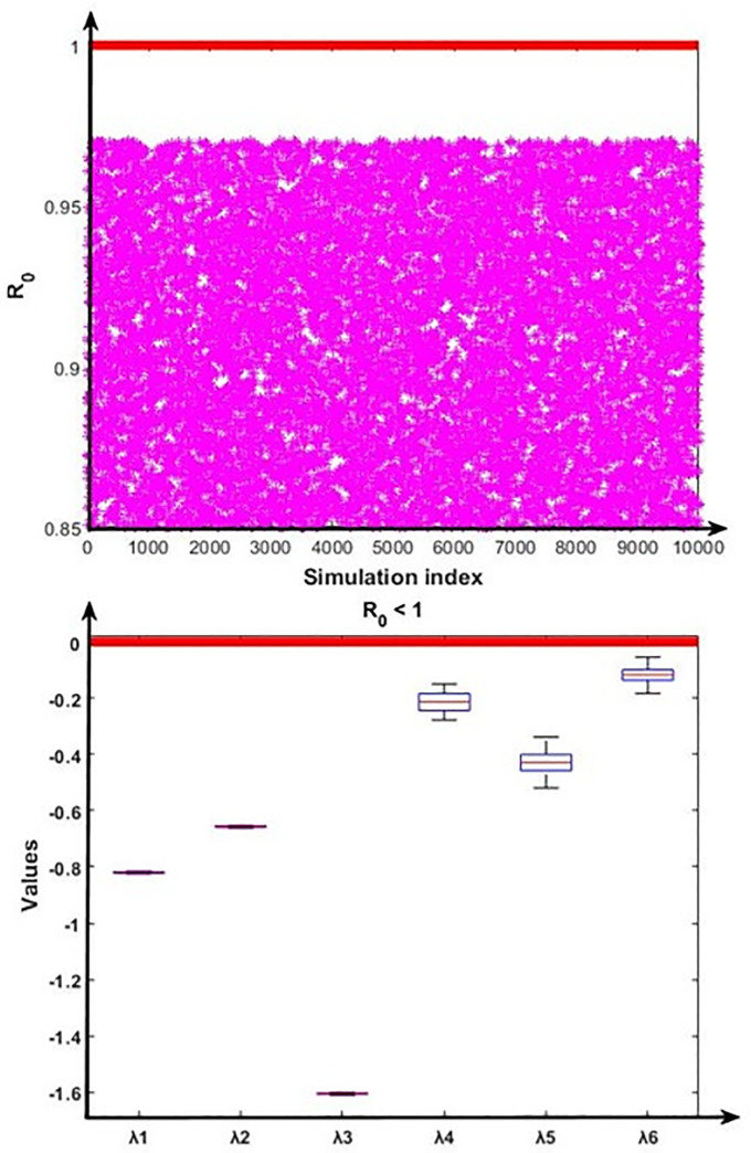
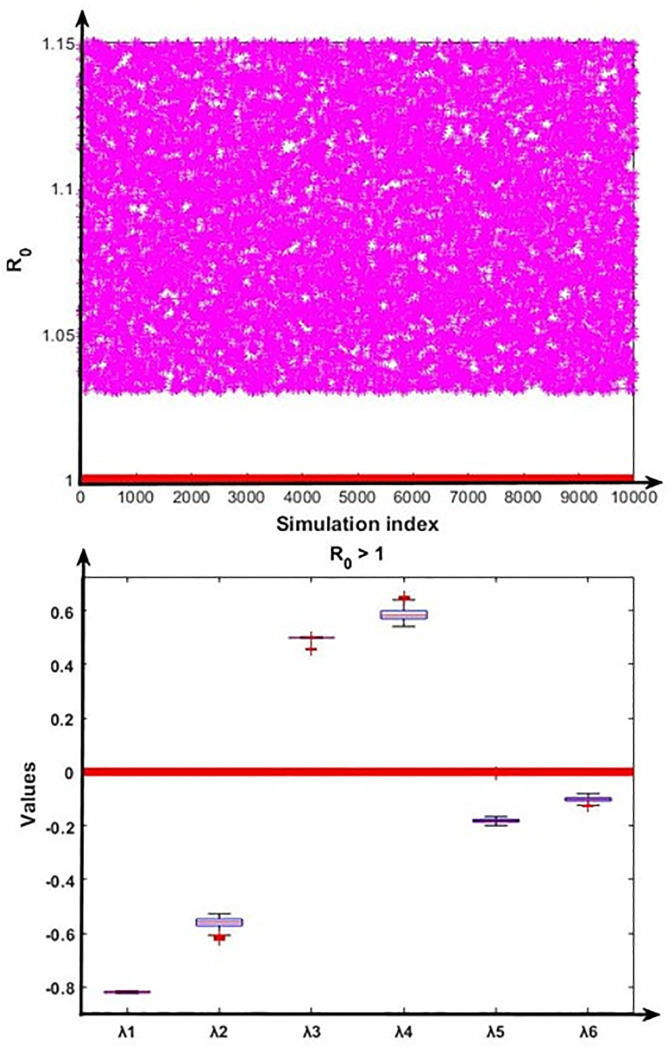
To validate the nature of the disease-free and endemic equilibrium analysis, we conducted the numerical analysis using the Monte Carlo simulation method [56] to verify the stability properties for the disease-free equilibrium and endemic equilibrium by calculating the fundamental part of the eigenvalues of the Jacobian matrix of the system (10)–(15). According to the disease-free equilibrium and disease endemic equilibrium, the steady states coordinates can be expressed in terms of fourteen model parameters (β, η, μ, ρ, σ, κ, α₁, α₂, ω₁, ω₂, ϕ, γ₁, γ₂, δ) whose baseline values are given in Table 1. The pool of sampling $\mathbb{N}={\prod }_{k=1}^{14}{A}_k\in {\mathbb{R}}_{+}^{14}$ was introduced by a Cartesian product of fourteen closed intervals of the form A_k = [a_k − θa_k, a_k + θa_k], where each a_k, k = 1, 2, ……14 stands for the baseline value of one parameter (see Table 1), and θ > 0 represents the range of variation. Our sampling comprised 10,000 confounding scenarios $N=(a_1,\dots \dots a_{14})\in \mathbb{N}$ where each a_k ∈ A_k, k = 1,2, ……14 was randomly chosen for θ = 0.20 (i.e., 20% deviation from the parameters baseline values) under a uniform distribution with no correlation between model parameters. The outcomes of this simulation are presented in Figs 2 and 3.

Fig 2. Numerical simulation for the stability condition of the disease-free equilibrium and the eigenvalues (λ₁, λ₂, λ₃, λ₄, λ₅ and λ₆) real part distribution.

First portion represents that R₀ < 1 always hold, and second portion depict the eigenvalues real part related distribution of the disease-free conditions.

Fig 3. Numerical analysis for the stability condition of the endemic equilibrium and the eigenvalues (λ₁, λ₂, λ₃, λ₄, λ₅ and λ₆) real part distribution.

First portion represents that R₀ < 1 always hold, and second portion depict the eigenvalues’ real part related distribution of the endemic equilibrium conditions.

Fig 2 displayed that the disease-free equilibrium is locally asymptotically stable as the real part of all six eigenvalues are negative (i.e. λ₁ < 0, λ₂ < 0, λ₃ < 0, λ₄ < 0, λ₅ < 0 and λ₆ < 0). Further, Fig 3 displayed that the endemic equilibrium is unstable as the real part of the two eigenvalues is positive (i.e. λ₃ > 0 and λ₄ > 0).

Estimation of parameters

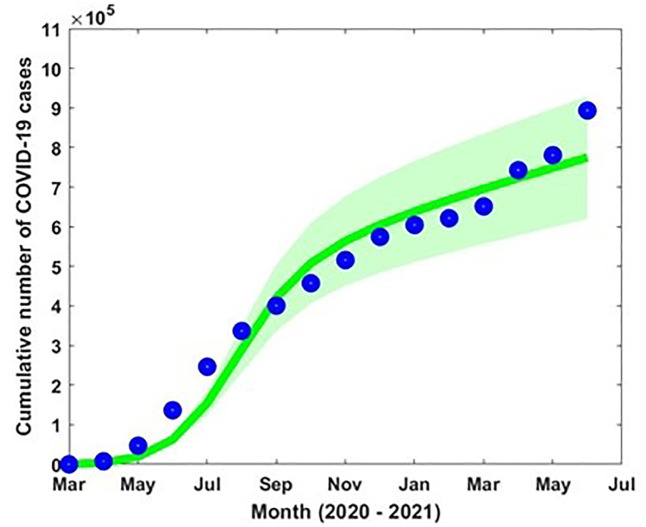
Model parameters are estimated based on the accessible COVID-19 data from March 2020 to June 2021 in Bangladesh [57]. The incidence of COVID-19 data in Bangladesh was available, and the number of cases increased from May to July (2020–2021) due to the outbreak of different variants. The transmission rate β, progression rate from L to M and C (ω₁ and ω₂) and loss of immunities (α₁ and α₂) are estimated by minimizing the error of the incidence data to the model curve using the least-squares fitting technique which offers a superior fit [56]. We used MATLAB optimization routine (built-in function such as ‘fmincon’) to perform least-square fitting for parameter estimation. The ‘fmincon’ is a MATLAB function used for solving constrained optimization problems. It stands for "function minimization with constraints" and is part of MATLAB’s Optimization Toolbox. Initial guess is considered for the parameters to optimize. This is a starting point for the algorithm to begin the search. Fig 4 shows the incidence data (blue dot) and the model-fitted curve (green solid curve) with the estimated parameter values β = 2.34 × 10⁻⁶, ω₁ = 0.013, ω₂ = 0.00731, α₁ = 0.0052, α₂ = 0.0203 and η = 1.124.

Fig 4. Reported COVID-19 incidence data (blue dots) and the model simulation (green solid curve), with the 95% confidence intervals (CI) indicated by the pink-shaded area.

In addition, the natural death rate (μ) was considered the inverse of the life expectancy (70 years) in Bangladesh. The rest of the parameter values were obtained from the literature (see Table 1).

The objective function used in the parameter estimation for the COVID-19 cumulative incidence is as follows:

$$\widehat{\theta }=\text{argmin}{\displaystyle {\sum }_{i=1}^n{\left(\left({\omega }_1+{\omega }_2\right){\text{L}}_{{\text{t}}_{\text{i}}}-{\text{data}}_{\text{tip}}\right)}^2}$$

where $\mathrm{d}\mathrm{a}\mathrm{t}{{\mathrm{a}}_{\mathrm{t}}}_{\mathrm{i}\mathrm{p}}$ represents the actual COVID-19 incidence data and $\left({\mathrm{\omega }}_1+{\mathrm{\omega }}_2\right){{\mathrm{L}}_{\mathrm{t}}}_{\mathrm{i}}$ is the corresponding model incidence solution at the time t_i and n is the number of available data points. The goal of the objective fuction is to minimize the sum of the squared differences (residuals) between the observed data and the model solution. The model (2)–(8) associated parameters are tabulated in Table 1.

Sensitivity analysis

Sensitivity analysis is a crucial modeling technique that evaluates how changes in important parameters impact the model’s results. Sensitivity analysis offers a methodical way to manipulate one or more parameters and track changes in the output to determine which parameters influence the model’s behaviour most. Here, we performed the sensitivity analysis of R₀ to the model parameters using the Latin Hypercube Sampling (LHS) method with 10000 runs per simulation. The LHS is a Monte Carlo stratified sampling method that allows us simultaneously to achieve an unbiased estimation of the model outcome for a specific set of input parameter values [51, 58, 59]. We allocated a uniform distribution for individual parameters from 0 to 4 times the baseline value.

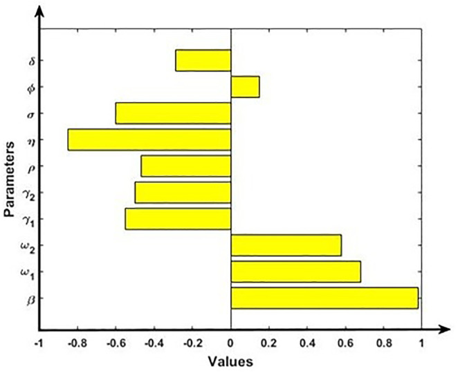
We calculate the Partial Rank Correlation Coefficients (PRCCs), a global sensitivity analysis technique of the key output variables. The PRCC positive value of model parameters indicates a positive correlation with model outputs and negative values represent a negative correlation. The PRCC for the full range of parameters is shown in the tornado plots in Fig 5. Results show that parameters β, ω₁, ω₂ and ϕ have a positive correlation with the effective reproduction number R₀, indicating that increasing the parameter values will increase the value of R₀. We found that transmission rate (β) has the high positive impact on effective reproduction number R₀. Hence, a small increase in the transmission rate can significantly raise the R₀, leading to a more rapid spread of the disease and higher peak infection rates. Conversely, a reduction in transmission rate (β) through interventions can flatten the epidemic curve. On the contrary, parameters γ₁, γ₂, ρ, η, σ, and δ have a negative association with the effective reproduction number R₀, implying that increasing the parameter values will reduce the value of R₀. Here, we found that first dose vaccination rate (η) has the high negative impact on R₀. Hence, the first does vaccination coverage rate significantly impacts herd immunity thresholds. Higher coverage rates lead to lower overall infection rates and can prevent outbreaks from reaching epidemic levels.

Fig 5. Sensitivity analysis of the model outcome R₀ and model parameters β, ω₁, ω₂, γ₁, γ₂, ρ, η, σ, ϕ and δ.

Bifurcation analysis

In this section, we present the bifurcation analysis of the proposed model (2)–(8) using the centre manifold theory as delineated by Castillo-Chavez and Song [60] (Theorem 4.1). We assume the bifurcation parameter as β, R₀ = 1, and then perform the bifurcation analysis [60–63]. We rewrite the model by considering S = x₁, V₁ = x₂, V₂ = x₃, L = x₄, M = x₅, C = x₆ as x = (x₁, x₂, x₃, x₄, x₅, x₆)^T, so the structure can be expressed as $\frac{\mathrm{d}\mathrm{x}}{\mathrm{d}\mathrm{t}}=\mathbf{f}\left(\mathrm{x}\right)$, where f = (f₁, f₂, f₃, f₄, f₅, f₆)^T.

Theorem 3

The model proposed in (2)–(8) has experienced backward bifurcation at β = β*, R₀ = 1. We provided the relative expression in the proof.

Proof:

Let consider S = x₁ and similarly, V₁ = x₂, V₂ = x₃, L = x₄, M = x₅, C = x₆. Then the system can be expressed as:

$$\begin{array}{ll}\frac{{\text{dx}}_1}{\text{dt}}=\hfill & \mu \text{N}+{\rho \text{x}}_2+{\delta \text{x}}_6-{\beta \text{x}}_1\left({\text{x}}_5+{\text{x}}_6\right)-{\text{v}}_1{\text{x}}_1\hfill \\ \frac{{\text{dx}}_2}{\text{dt}}=\hfill & {\beta \text{x}}_1-{\text{v}}_2{\text{x}}_2\hfill \\ \frac{{\text{dx}}_3}{\text{dt}}=\hfill & {\sigma \text{x}}_2-{\text{v}}_3{\text{x}}_3\hfill \\ \frac{{\text{dx}}_4}{\text{dt}}=\hfill & {\beta \text{x}}_1\left({\text{x}}_5+{\text{x}}_6\right)+{\alpha }_1{\text{x}}_2+{\alpha }_2{\text{x}}_3-{\text{v}}_4{\text{x}}_4\hfill \\ \frac{{\text{dx}}_5}{\text{dt}}=\hfill & {\omega }_1{\text{x}}_4-{\text{v}}_5{\text{x}}_5\hfill \\ \frac{{\text{dx}}_6}{\text{dt}}=\hfill & {\omega }_2{\text{x}}_4+\varphi {\text{x}}_5-{\text{v}}_6{\text{x}}_6\hfill \end{array}$$ (20)

Here, v₁ = (η + μ), v₂ = (ρ + σ + α₁ + μ), v₃ = (κ + α₂ + μ), v₄ = (ω₁ + ω₂ + μ), v₅ = (γ₁ + ϕ + μ), v₆ = (γ₂ + δ + μ), and v₇ = u₁u₂–ηρ. The transmission rate among the susceptible, unvaccinated group is defined as the bifurcation parameter, with the condition R₀ = 1. Thus, we have

$${\beta }^{*}=\frac{\left(\left(\mathrm{\rho }+\mathrm{\sigma }++\mathrm{\mu }\right)\left(\mathrm{\eta }+\mathrm{\mu }\right)-\mathrm{\eta }\mathrm{\rho }\right)\left({\mathrm{\omega }}_1+{\mathrm{\omega }}_2+\mathrm{\mu }\right)\left(\varphi +{\mathrm{\gamma }}_1+\mathrm{\mu }\right)\left({\mathrm{\gamma }}_2+\delta +\mathrm{\mu }\right)}{\mathrm{\mu }\mathrm{N}\left(\mathrm{\rho }+\mathrm{\sigma }+{\mathrm{\alpha }}_1+\mathrm{\mu }\right)\left[{\mathrm{\omega }}_1\left(\varphi +{\mathrm{\gamma }}_2+\delta +\mathrm{\mu }\right)+{\mathrm{\omega }}_2\left(\varphi +{\mathrm{\gamma }}_1+\mathrm{\mu }\right)\right]}$$ (21)

So the disease-free equilibrium point for the transformed system (20) is,

$${\mathrm{E}}^0=\left({\mathrm{x}}_1^0,{\mathrm{x}}_2^0,{\mathrm{x}}_3^0,{\mathrm{x}}_4^0,{\mathrm{x}}_5^0,{\mathrm{x}}_6^0\right)=\left(\frac{{\mathrm{v}}_2\mathrm{N}\mathrm{\mu }}{{\mathrm{v}}_7},\frac{\mathrm{N}\mathrm{\mu }\mathrm{\eta }}{{\mathrm{v}}_7},\frac{\mathrm{N}\mathrm{\mu }\mathrm{\eta }\mathrm{\sigma }}{{\mathrm{v}}_7},\mathrm{0,0},0\right)$$

The linearization matrix of the transformed system (20), can be expressed in terms of Jacobian as J(E⁰):

$$\text{J}\left({\text{E}}^0\right)=\left[\begin{array}{cccccc}-{\text{v}}_1& \rho & 0& 0& -\beta \frac{{\text{v}}_2\text{N}\mu }{{\text{v}}_7}& -\beta \frac{{\text{v}}_2\text{N}\mu }{{\text{v}}_7}+\delta \\ \eta & -{\text{v}}_2& 0& 0& 0& 0\\ 0& \sigma & -{\text{v}}_3& 0& 0& 0\\ 0& {\alpha }_1& {\alpha }_2& -{\text{v}}_4& \beta \frac{{\text{v}}_2\text{N}\mu }{{\text{v}}_7}& \beta \frac{{\text{v}}_2\text{N}\mu }{{\text{v}}_7}\\ 0& 0& 0& {\omega }_1& -{\text{v}}_5& 0\\ 0& 0& 0& {\omega }_2& \varphi & -{\text{v}}_6\end{array}\right]$$ (22)

When, R₀ = 1, i.e., at β*, the expressed Jacobian (22) of the system possesses a single zero eigenvalue, and the remaining eigenvalues exhibit negative real parts. Consequently, the behavior of the transformed system in the vicinity of β* (at R₀ = 1) is analyzed through the application of central manifold theory [60]. The essential computations based on the central manifold theory [60–63] are outlined as follows. Let. H = (h_1, h_2, h_3, h_4, h_5, h₆)^T be the right eigenvector for J(E⁰) at R₀ = 1, is determined by solving J(E⁰).H = 0, and therefore

$${\mathrm{h}}_1=\frac{{\mathrm{h}}_2\left(\begin{array}{c}\left(\left({\mathrm{\alpha }}_1+\mathrm{\rho }\right){\mathrm{v}}_3+{\mathrm{\alpha }}_2\mathrm{\sigma }\right)\mathrm{\mu }\mathrm{\beta }\left(\left({\mathrm{v}}_6+\varphi \right){\mathrm{\omega }}_1+{{\mathrm{v}}_5\mathrm{\omega }}_2\right)\mathrm{N}{\mathrm{v}}_2\\ -{\mathrm{v}}_7\left(\varphi \delta \left({\mathrm{\alpha }}_2\mathrm{\sigma }+{{\mathrm{\alpha }}_1\mathrm{v}}_3\right){\mathrm{\omega }}_1+\left(\left({\delta {\mathrm{\alpha }}_1\mathrm{\omega }}_2+\mathrm{\rho }{\mathrm{v}}_4{\mathrm{v}}_6\right){\mathrm{v}}_3+{\mathrm{\alpha }}_2\mathrm{\sigma }{\delta \mathrm{\omega }}_2\right){\mathrm{v}}_5\right)\end{array}\right)}{{\mathrm{v}}_1{\mathrm{v}}_3\left(\mathrm{\mu }\beta \left(\left({\mathrm{v}}_6+\varphi \right){\mathrm{\omega }}_1+{{\mathrm{v}}_5\mathrm{\omega }}_2\right)\mathrm{N}{\mathrm{v}}_2-{\mathrm{v}}_4{\mathrm{v}}_5{\mathrm{v}}_6{\mathrm{v}}_7\right)},$$

$${\mathrm{h}}_3=\frac{{\mathrm{h}}_2\mathrm{\sigma }}{{\mathrm{v}}_3},{\mathrm{h}}_4=\frac{{\mathrm{h}}_2{\mathrm{v}}_5{\mathrm{v}}_6{\mathrm{v}}_7\left({\mathrm{\alpha }}_2\mathrm{\sigma }+{{\mathrm{\alpha }}_1\mathrm{v}}_3\right)}{{\mathrm{v}}_3\left(-\mathrm{\mu }\beta \left(\left({\mathrm{v}}_6+\varphi \right){\mathrm{\omega }}_1+{{\mathrm{v}}_5\mathrm{\omega }}_2\right)\mathrm{N}{\mathrm{v}}_2+{\mathrm{v}}_4{\mathrm{v}}_5{\mathrm{v}}_6{\mathrm{v}}_7\right)},$$

$${\mathrm{h}}_5=\frac{{\mathrm{h}}_2{\mathrm{\omega }}_1{\mathrm{v}}_6{\mathrm{v}}_7\left({\mathrm{\alpha }}_2\mathrm{\sigma }+{{\mathrm{\alpha }}_1\mathrm{v}}_3\right)}{{\mathrm{v}}_3\left(-\mathrm{\mu }\beta \left(\left({\mathrm{v}}_6+\varphi \right){\mathrm{\omega }}_1+{{\mathrm{v}}_5\mathrm{\omega }}_2\right)\mathrm{N}{\mathrm{v}}_2+{\mathrm{v}}_4{\mathrm{v}}_5{\mathrm{v}}_6{\mathrm{v}}_7\right)},$$

$${\mathrm{h}}_6=\frac{{\mathrm{h}}_2\left(\varphi {\mathrm{\omega }}_1+{{\mathrm{v}}_5\mathrm{\omega }}_2\right){\mathrm{v}}_7\left({\mathrm{\alpha }}_2\mathrm{\sigma }+{{\mathrm{\alpha }}_1\mathrm{v}}_3\right)}{{\mathrm{v}}_3\left(-\mathrm{\mu }\beta \left(\left({\mathrm{v}}_6+\varphi \right){\mathrm{\omega }}_1+{{\mathrm{v}}_5\mathrm{\omega }}_2\right)\mathrm{N}{\mathrm{v}}_2+{\mathrm{v}}_4{\mathrm{v}}_5{\mathrm{v}}_6{\mathrm{v}}_7\right)}.$$

Let. K = (k_1, k_2, k_3, k_4, k_5, k₆)^T be the left eigenvector for J(E⁰) at R₀ = 1, is determined by solving K.J(E⁰) = 0 (calculated by J(E⁰)^T. K), and therefore we have,

$${\mathrm{k}}_1=\frac{\mathrm{\eta }{\mathrm{k}}_2}{{\mathrm{v}}_1},{\mathrm{k}}_3=\frac{\mathrm{\eta }{\mathrm{k}}_2{\mathrm{\alpha }}_2\left(\mathrm{\mu }\left(\left({\mathrm{v}}_6+\varphi \right){\mathrm{\omega }}_1+{{\mathrm{v}}_5\mathrm{\omega }}_2\right)\beta \mathrm{N}{\mathrm{v}}_2-\delta {\mathrm{v}}_7\left(\varphi {\mathrm{\omega }}_1+{{\mathrm{v}}_5\mathrm{\omega }}_2\right)\right)}{{\mathrm{v}}_1{\mathrm{v}}_3\left(\mathrm{\mu }\beta \left(\left({\mathrm{v}}_6+\varphi \right){\mathrm{\omega }}_1+{{\mathrm{v}}_5\mathrm{\omega }}_2\right)\mathrm{N}{\mathrm{v}}_2-{\mathrm{v}}_4{\mathrm{v}}_5{\mathrm{v}}_6{\mathrm{v}}_7\right)},$$

$${\mathrm{k}}_4=\frac{\mathrm{\eta }{\mathrm{k}}_2\left(\mathrm{\mu }\left(\left({\mathrm{v}}_6+\varphi \right){\mathrm{\omega }}_1+{{\mathrm{v}}_5\mathrm{\omega }}_2\right)\beta \mathrm{N}{\mathrm{v}}_2-\delta {\mathrm{v}}_7\left(\varphi {\mathrm{\omega }}_1+{{\mathrm{v}}_5\mathrm{\omega }}_2\right)\right)}{{\mathrm{v}}_1\left(\mathrm{\mu }\beta \left(\left({\mathrm{v}}_6+\varphi \right){\mathrm{\omega }}_1+{{\mathrm{v}}_5\mathrm{\omega }}_2\right)\mathrm{N}{\mathrm{v}}_2-{\mathrm{v}}_4{\mathrm{v}}_5{\mathrm{v}}_6{\mathrm{v}}_7\right)},$$

$${\mathrm{k}}_5=\frac{\mathrm{\eta }{\mathrm{k}}_2\left(\mathrm{\mu }\left(\left({\mathrm{v}}_6+\varphi \right){\mathrm{v}}_4-{\delta \mathrm{\omega }}_2\right)\beta \mathrm{N}{\mathrm{v}}_2-\delta {\varphi {\mathrm{v}}_4\mathrm{v}}_7\right)}{{\mathrm{v}}_1{\mathrm{v}}_3\left(\mathrm{\mu }\beta \left(\left({\mathrm{v}}_6+\varphi \right){\mathrm{\omega }}_1+{{\mathrm{v}}_5\mathrm{\omega }}_2\right)\mathrm{N}{\mathrm{v}}_2-{\mathrm{v}}_4{\mathrm{v}}_5{\mathrm{v}}_6{\mathrm{v}}_7\right)},$$

$${\mathrm{k}}_6=\frac{\mathrm{\eta }{\mathrm{k}}_2\left(\beta \mathrm{N}{\mathrm{v}}_2\mathrm{\mu }\left(\delta {\mathrm{\omega }}_1+{\mathrm{v}}_4{\mathrm{v}}_5\right)-\delta {\mathrm{v}}_4{\mathrm{v}}_5{\mathrm{v}}_7\right)}{{\mathrm{v}}_1\left(\mathrm{\mu }\beta \left(\left({\mathrm{v}}_6+\varphi \right){\mathrm{\omega }}_1+{{\mathrm{v}}_5\mathrm{\omega }}_2\right)\mathrm{N}{\mathrm{v}}_2-{\mathrm{v}}_4{\mathrm{v}}_5{\mathrm{v}}_6{\mathrm{v}}_7\right)}.$$

Subsequently, k₂ is computed to satisfy the requirement that H.K = 1⁵⁶, thus resulting in k₂ = 1, whereas h₂ can be expressed as:

$${\text{h}}_2=\frac{1}{\left(\begin{array}{c}1+\frac{\eta \left(\begin{array}{c}\left(\left({\alpha }_1+\rho \right){\text{v}}_3+{\alpha }_2\sigma \right)\mathrm{\mu }\mathrm{\beta }\left(\left({\text{v}}_6+\varphi \right){\omega }_1+{\text{v}}_5{\omega }_2\right)\mathrm{N}{\text{v}}_2\\ -{\text{v}}_7\left(\varphi \delta \left({\alpha }_2\sigma +{\alpha }_1{\text{v}}_3\right){\omega }_1+\left(\left({\delta \alpha }_1{\omega }_2+{\rho \text{v}}_4{\text{v}}_6\right){\text{v}}_3+{\alpha }_2{\sigma \delta \omega }_2\right){\text{v}}_5\right)\end{array}\right)}{{\text{v}}_1{\text{v}}_3\left(\mu \beta \left(\left({\text{v}}_6+\varphi \right){\omega }_1+{\text{v}}_5{\omega }_2\right){\text{Nv}}_2-{\text{v}}_4{\text{v}}_5{\text{v}}_6{\text{v}}_7\right){\text{v}}_1}\\ +\frac{{\eta \alpha }_2\sigma \left(\mu \left(\left({\text{v}}_6+\varphi \right){\omega }_1+{\text{v}}_5{\omega }_2\right){\beta \text{Nv}}_2-{\delta \text{v}}_7\left(\varphi {\omega }_1+{\text{v}}_5{\omega }_2\right)\right)}{{\text{v}}_1{\text{v}}_3\left(\mu \beta \left(\left({\text{v}}_6+\varphi \right){\omega }_1+{\text{v}}_5{\omega }_2\right){\text{Nv}}_2-{\text{v}}_4{\text{v}}_5{\text{v}}_6{\text{v}}_7\right){\text{v}}_3}\\ -\frac{\eta \left({\text{v}}_5{\text{v}}_6{\text{v}}_7\left({\alpha }_2\sigma +{\alpha }_1{\text{v}}_3\right)\right)\left(\mu \left(\left({\text{v}}_6+\varphi \right){\omega }_1+{\text{v}}_5{\omega }_2\right){\beta \text{Nv}}_2-{\delta \text{v}}_7\left(\varphi {\omega }_1+{\text{v}}_5{\omega }_2\right)\right)}{{\text{v}}_1{\text{v}}_3{\left(\mu \beta \left(\left({\text{v}}_6+\varphi \right){\omega }_1+{\text{v}}_5{\omega }_2\right){\text{Nv}}_2-{\text{v}}_4{\text{v}}_5{\text{v}}_6{\text{v}}_7\right)}^2}\\ -\frac{\eta \left({\omega }_1{\text{v}}_6{\text{v}}_7\left({\alpha }_2\sigma +{\alpha }_1{\text{v}}_3\right)\right)\left(\mu \left(\left({\text{v}}_6+\varphi \right){\text{v}}_4-{\delta \omega }_2\right){\beta \text{Nv}}_2-\delta \varphi {\text{v}}_4{\text{v}}_7\right)}{{\text{v}}_3{\text{v}}_1{\text{v}}_3{\left(\mu \beta \left(\left({\text{v}}_6+\varphi \right){\omega }_1+{\text{v}}_5{\omega }_2\right){\text{Nv}}_2-{\text{v}}_4{\text{v}}_5{\text{v}}_6{\text{v}}_7\right)}^2}\\ -\frac{{\eta \text{v}}_7\left({\beta \text{Nv}}_2\mu \left({\delta \omega }_1+{\text{v}}_4{\text{v}}_5\right)-{\delta \text{v}}_4{\text{v}}_5{\text{v}}_7\right)\left(\varphi {\omega }_1+{\text{v}}_5{\omega }_2\right)\left({\alpha }_2\sigma +{\alpha }_1{\text{v}}_3\right)}{{\text{v}}_1{\text{v}}_3{\left(\mu \beta \left(\left({\text{v}}_6+\varphi \right){\omega }_1+{\text{v}}_5{\omega }_2\right){\text{Nv}}_2-{\text{v}}_4{\text{v}}_5{\text{v}}_6{\text{v}}_7\right)}^2}\end{array}\right)},$$

So, the bifurcation coefficient a and b can be written as^55,56,57,58,

$$a={\displaystyle \sum }_{\text{p},\text{q},\text{r}=1}^6{\text{k}}_{\text{r}}{\text{h}}_{\text{p}}{\text{h}}_{\text{q}}\frac{{\partial }^2{\text{f}}_{\text{r}}\left({\text{E}}^0,{\beta }^{*}\right)}{\partial {\text{x}}_{\text{p}}\partial {\text{x}}_{\text{q}}}\text{and}b={\displaystyle \sum }_{\text{p},\text{q},\text{r}=1}^6{\text{k}}_{\text{r}}{\text{h}}_{\text{p}}\frac{{\partial }^2{\text{f}}_{\text{r}}\left({\text{E}}^0,{\beta }^{*}\right)}{\partial {\text{x}}_{\text{p}}\partial \beta }.$$ (23)

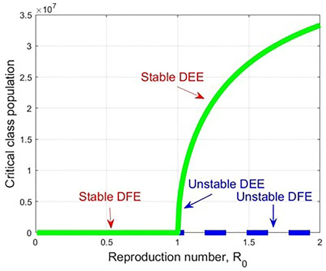
By substituting the corresponding values of H = (h_1, h_2, h_3, h_4, h_5, h₆), K = (k_1, k_2, k_3, k_4, k_5, k₆), and performing the partial derivative of the transformed function (f_l(E⁰, β*)), putting the corresponding rate parameter values, we observe the forward bifurcation at R₀ = 1. In the forward bifurcation case, the disease-free equilibrium becomes unstable, and the disease-endemic equilibrium point becomes stable when R₀ >1 (see Fig 6). Forward bifurcation provides a clear and predictable threshold behaviour at R₀ = 1, making it easy to determine whether COVID-19 will die out or become endemic. It indicates that maintaining R₀ below 1 is sufficient to eliminate the disease. This insight helps in designing control strategies that are focused on reducing R₀ through vaccination, social distancing, or other interventions.

Fig 6. A forward bifurcation graph which displays the stability changes concerning R₀, when R₀ ranges from 0 to 2.

Numerical simulation

In this section, we carry out detailed numerical simulations using the MATLAB programming language to support the analytic results and measure the effect of first and second-dose vaccination and different biological parameters on the proposed COVID-19 model in Bangladesh. MATLAB’s powerful numerical solvers and visualization tools make it ideal for analyzing the behavior of epidemic models across various domains. We used the MATLAB toolbox to solve ordinary differential equations (ODEs). It has built-in functions like ‘ode45’ for solving ODEs of our proposed model. For illustration, we have chosen baseline parameter values consistent with COVID-19 infection and transmission. By the analytic results, we found two equilibrium points: the infection-free equilibrium (E⁰); and disease endemic equilibrium(E*). Furthermore, we employed various initial conditions for all populations and established that if R₀ is less than one, then the infection-free equilibrium is locally asymptotically stable. Further, if R₀ is greater than one, then the COVID-19 disease persists in the population.

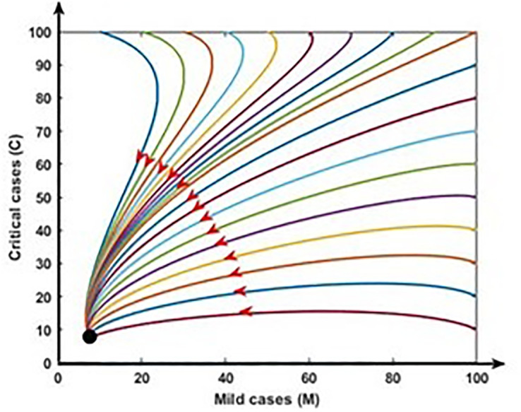
Fig 7 demonstrates the stability of the infection-free equilibrium (i.e., R₀ < 1) by illustrating model trajectories through the M vs C plane starting for various initial conditions. In such a case, COVID-19 fade-out. Fig 8 shows the stability of the endemic equilibrium (i.e., R₀ > 1), and in that event, COVID-19 disease persists in the population.

Fig 7. Disease free equilibrium: R₀ < 1. In this case COVID-19 fade-out (black dot).

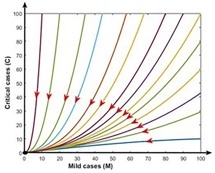
Fig 8. Endemic equilibrium: R₀ > 1. In this case COVID-19 persist in the population (black dot).

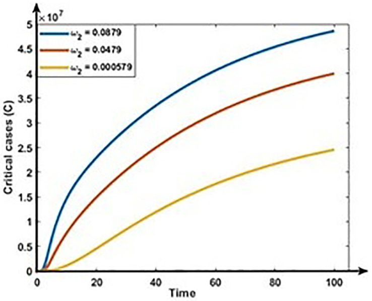
Figs 9 and 10 show the impact of progression rates (ω₁ and ω₂) on the dynamics of Mild and Critical cases. From these Figures, we perceive that the burden of Mild and Critical cases increases if the progression rates rise, which means those positively associated with Mild and Critical cases.

Fig 9. Impact of progression rate (ω₁) on the dynamics of Mild cases (M).

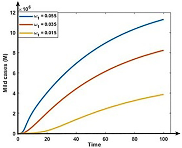
Fig 10. Impact of progression rate (ω₂)on the dynamics of Critical cases (C).

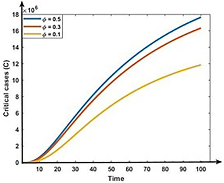
Figs 11 and 12 show the impact of co-infection rate on the dynamics of Mild and Critical cases. Results show that the co-infection rate negatively correlates with Mild cases but positively correlates with Critical cases. Our analysis is consistent with reality because the following infection, some Mild populations move to the critical cases due to the co-infection with other diseases, including hypertension, diabetes, cardiovascular disease, and respiratory disease.

Fig 11. Impact of co-infection rate (ϕ) on the dynamics of Mild cases (M).

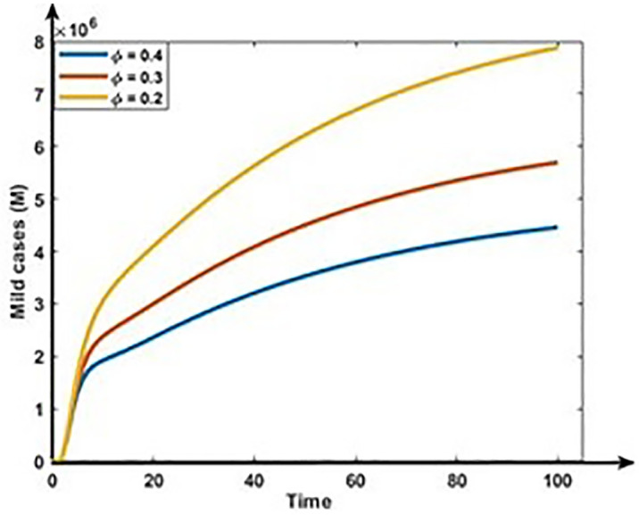
Fig 12. Impact of co-infection rate (ϕ) on the dynamics of Critical cases (C).

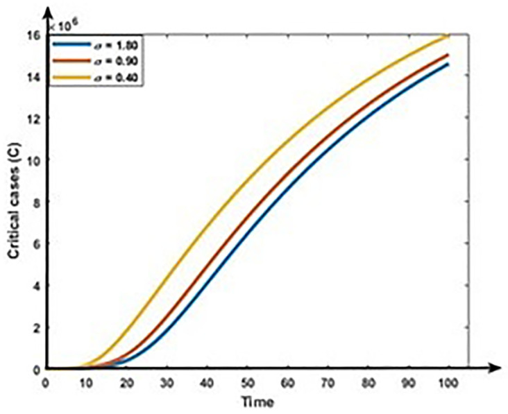
Figs 13 and 14 show that the rises in the first dose vaccination rates decrease the Mild and Critical cases of COVID-19 and decrease the risk of an outbreak. Figs 15 and 16 display that the rise in the second dose vaccination rates declines the Mild and Critical cases of COVID-19 in Bangladesh. From this analysis, we observe that the First-dose vaccination rate has a higher impact on COVID-19 cases compared to the second-dose vaccination rate, which is consistent with our observation and previous study [64] because the first-dose vaccine may prevent transmission from an infected person to another person.

Fig 13. Impact of first does vaccination rate (η) on the dynamics of Mild cases (M).

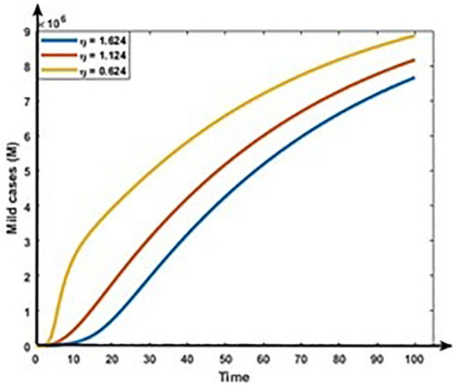
Fig 14. Impact of first does vaccination rate (η) on the dynamics of Critical cases (C).

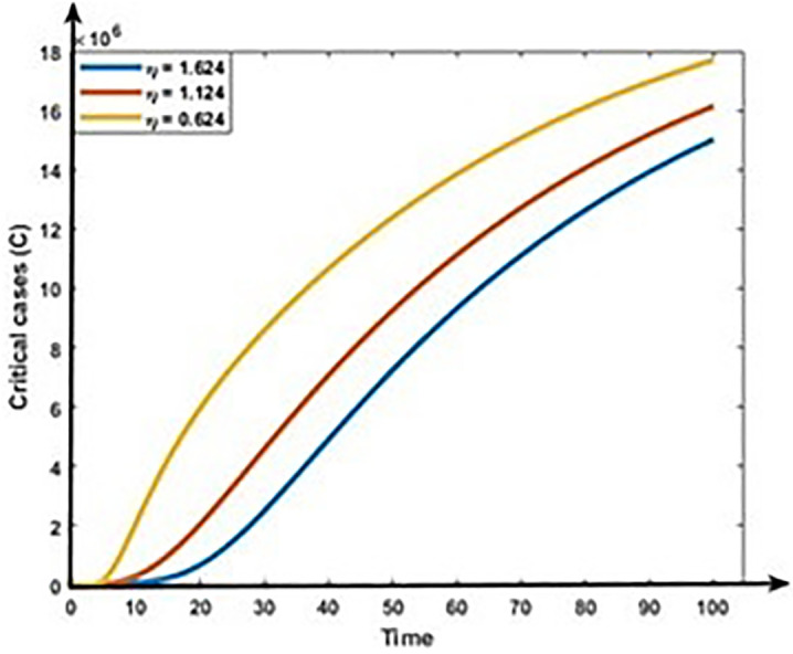
Fig 15. Impact of second does vaccination rate (σ) on the dynamics of Mild cases (M).

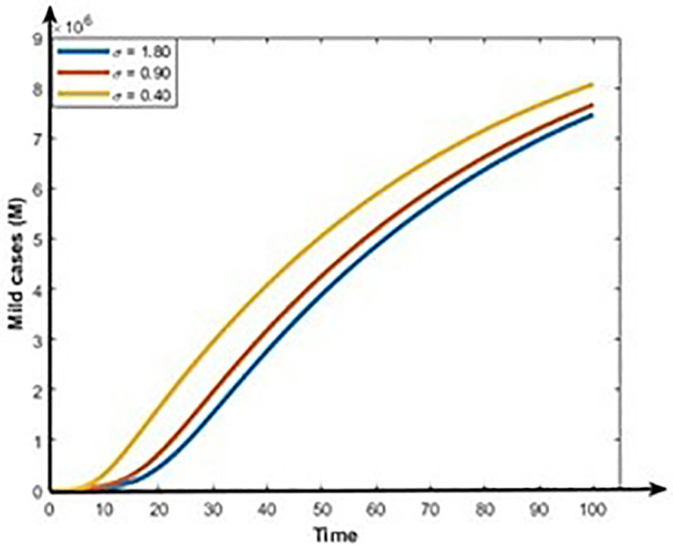
Fig 16. Impact of second does vaccination rate (σ) on the dynamics of Critical cases (C).

Discussion and conclusion

In this paper, we proposed a seven-compartmental COVID-19 model by introducing the epidemiology of mild and critical cases with dual-dose vaccination in Bangladesh. We analyzed that the solutions of this model are bounded and non-negative. We also determined a mathematical expression for the effective reproduction number of the model to confirm whether this disease persists or dies out. We found that if R₀ is less than one, i.e., R₀ < 1, the disease-free equilibrium is locally asymptotically stable. Conversely, if R₀ is greater than one, i.e., R₀ > 1, the coronavirus infection persists in the population. This analysis can help us to identify regions in the parameter space where the various asymptotic states are stable or unstable, thus allowing us to predict the long-term behavior of the COVID-19 dynamics. This information can advise the Ministry of Health in Bangladesh to reduce the period of infectiousness until R₀ < 1.

The existence and stability of the transmission dynamics of nonlinear COVID-19 models were considered in previous modeling studies [45, 46, 65–68]. Previous studies show that if the effective reproduction number is less than one, the COVID-19 disease dies out of the community. On the other hand, if the effective reproduction number is greater than one, the disease persists in the community [45, 46, 66, 67], which is similar to our results. Numerous COVID-19 modelling studies examined the effect of different intervention scenarios. Results show that combined intervention strategies are the most effective for reducing the burden of COVID-19. In this study, we considered Bangladesh-specific seven compartmental COVID-19 model and allowed the Mild class population to move to the Critical class due to the co-infection and comorbidity with other diseases, including diabetes, cardiovascular disease, chronic respiratory disease, and cancer are more likely to develop a serious illness which is not considered in previous modeling studies [46, 48].

To investigate the significance of the model parameters, we implemented the sensitivity analysis of the effective reproduction number R₀ corresponding to the model parameters. The result shows that transmission rate β is the most significant parameter, which is because infectious COVID-19 patients transmit the disease through coughing, sneezing, and spitting are the main source of infection, which is consistent with previous modeling studies [36, 49, 58, 65]. If the inhaled coronavirus enters and settles in the body of a healthy person and begins to multiple infection. Therefore, it is crucial to defend susceptible persons from COVID-19 infected person from a public health viewpoint by efficiently dropping the transmission rate between susceptible and infectious persons. In addition, the degree of exposure to this disease is extensive for those who are in close and prolonged contact with an infectious individual. Hence, it is very important to identify and notify individuals who have been in contact with infected persons to break the chain of transmission. Controlling the transmission of COVID-19 involves implementing a combination of public health measures and individual behaviors to reduce the spread of the virus. The second most important parameter is the first dose vaccination rate η, which is because it prevents the spread of contagious and dangerous. WHO stated that vaccination not only protects vaccinated persons, it also reduces exposure in the community. Therefore, increasing completion of vaccination rate is the most effective way of preventing COVID-19 disease in Bangladesh.

Qualitative techniques are important to understand real-world phenomena, which offer valuable insights into public hesitancy, misinformation, cultural beliefs, and barriers to vaccination that quantitative methods often overlook. Understanding these factors is essential for developing effective communication strategies and interventions to enhance vaccine uptake in Bangladesh. Meanwhile, bifurcation analysis identifies critical points where minor changes in vaccination rates or public health measures can cause major shifts in disease dynamics, such as transitioning from a controlled outbreak to an epidemic or vice versa. This information is crucial for determining when to adjust vaccination strategies or modify public health measures.

Integrating qualitative and bifurcation analysis enables a comprehensive understanding of both social dynamics and the mathematical modeling of disease transmission. This interdisciplinary approach combines insights from social sciences and epidemiological modeling, improving the reliability of results by considering multiple dimensions of the problem. Justifying the use of both methodologies bridges the gap between theoretical modeling and practical realities, which is key for translating insights into actionable public health strategies in Bangladesh.

Determining the effective reproduction number can help public health officials focus vaccination efforts on areas with higher transmission rates. Our study’s insights into factors affecting transmission, such as co-infection, vaccination, and progression rates, can inform the design of public health interventions tailored to specific local contexts. Additionally, findings from bifurcation and stability analyses can guide policymakers on when to adjust control measures like lockdowns, social distancing, or mask mandates based on real-time data, thereby minimizing COVID-19 spread and reducing the socio-economic impact of extended restrictions. The study identifies key parameters, such as vaccination and transmission rates, significantly affecting disease dynamics. Public health authorities can use this information to allocate vaccines more effectively, prioritizing high-risk groups or areas with high transmission. This study also guides policymakers in adjusting strategies like testing, contact tracing, quarantine, or social distancing by pinpointing critical points where small changes in vaccination or health measures impact transmission. Additionally, the findings support contingency planning by anticipating scenarios where new variants with different transmission rates could arise.

From the numerical analysis, it is also clear that an increment in the vaccine dose rate reduces the spread of COVID-19, which is similar to the previous study [64]. Therefore, to control and eradicate COVID-19 infection, it is vital to consider the following policies: (a) the first and most significant policy is to reduce the transmission rate with infected people; (b) the second most significant policy is to raise the vaccination rate. Therefore, we recommended that the most feasible and optimal strategy to eliminate COVID-19 in Bangladesh is to decrease the transmission rate through a mass vaccination campaign to cover most of the total population vaccination as soon as possible. There are many ways we can minimize the transmission rate, such as personal respiratory protection; this includes wearing masks by patients to reduce the dispersal of coronavirus when they talk, cough, or sneeze. Moreover, patients must be taught basic infection control measures, such as covering the nose and mouth during coughing.

Ongoing research is crucial for developing and improving new vaccines, especially as the virus evolves with new variants. This includes studying long-term immunity, booster needs, and vaccine efficacy against emerging strains. To lessen the severity of COVID-19 infections and avoid fatalities, research into antiviral medications, monoclonal antibodies, and other therapies is still essential. This involves exploring alternative applications for already-approved medications and creating novel treatments based on the most recent research. International collaboration ensures equitable vaccine access, especially in low- and middle-income countries, including Bangladesh. Sharing epidemiological data and research findings across countries and institutions accelerates the global response to COVID-19. Collaborative research projects across borders have led to rapid advancements in understanding COVID-19, from vaccine development to public health strategies.

To balance the need to manage the virus and limit economic and social disturbance, decisions on public health measures, such as lockdowns, mask requirements, and travel restrictions, must be supported by scientific data. Governments may preserve public health and consider broader social effects by using evidence-based recommendations to guide their decision-making. In addition, stakeholders, policymakers, and researchers may all work together to improve the efficacy of the worldwide response to COVID-19 by utilizing study findings. Continued collaboration, informed decision-making, and translating research into practice are crucial to overcoming the challenges of the pandemic and preparing for future public health emergencies.

Limitations

It is important to note that this study has several limitations. First, a homogeneous mixed population model was taken into consideration. Homogeneous models ignore variances in factors like age, behavior, health, and economic status, presuming uniformity throughout the population. These differences can substantially impact the dynamics of disease transmission, the results of treatments, and the efficacy of interventions. By including heterogeneous features into modeling techniques, public health policies may better accommodate the different requirements of the community while also improving forecast precision. Under-reporting and misclassification cases of COVID-19 occur in Bangladesh due to inadequate recognition of infectious disease surveillance, nonspecific COVID-19 symptoms, and restricted access to healthcare facilities, and bias cannot be completely eliminated. Therefore, more accurate data should be gathered in order to solve COVID-19-related difficulties. Before putting our findings into practice, policymakers must take data into consideration, as our suggested results are dependent on it. In future, we will develop a heterogeneous population model to explore how factors like age, health status, occupation and behaviour interact with COVID-19. We will also identify which subgroups are most at risk and design vaccination and targeted interventions.

Supporting information

S1 Data

(XLSX)

Data Availability

All relevant data are within the manuscript and its Supporting information files.

Funding Statement

The author(s) received no specific funding for this work.

References

- 1.Sehgal M., Ladd J.H., Totapally B.: Trends in epidemiology and microbiology of severe sepsis and septic shock in children. Hosp Pediatr. 10(12), 1021–1030 (2020). doi: 10.1542/hpeds.2020-0174 [DOI] [PubMed] [Google Scholar]
- 2.World Health Organization (WHO). WHO reveals leading causes of death and disability worldwide: 2000–2019, (2020).
- 3.Harbeck M., Seifert L., Hänsch S., Wagner D.M., Birdsell D., Parise K.L., et al.: Yersinia pestis DNA from skeletal remains from the 6th century AD reveals insights into Justinianic Plague. PLoS pathog. 9(5), e1003349 (2013). doi: 10.1371/journal.ppat.1003349 [DOI] [PMC free article] [PubMed] [Google Scholar]
- 4.World Health Organization. (2023). COVID-19 Dashboard. https://covid19.who.int.
- 5.Zhang T., Qiao J., Hayashi K., & Nishiura H. (2024). Decomposing mechanisms of COVID-19 mortality in empirical datasets: A modeling study. Journal of Theoretical Biology, 584, 111771. doi: 10.1016/j.jtbi.2024.111771 [DOI] [PubMed] [Google Scholar]
- 6.Huang C., Wang Y., Li X., Ren L., Zhao J., Hu Y., et al.: Clinical features of patients infected with 2019 novel coronavirus in Wuhan, China. Lancet. 395(10223), 497–506 (2020). [DOI] [PMC free article] [PubMed] [Google Scholar]
- 7.Shahrear P., Rahman S.S., Nahid M.M.H.: Prediction and mathematical analysis of the outbreak of coronavirus (COVID-19) in Bangladesh. Results App. Math. 10, 100145 (2021). doi: 10.1016/j.rinam.2021.100145 [DOI] [PMC free article] [PubMed] [Google Scholar]
- 8.Kabir M.H., Gani M.O., Mandal A., Biswas M.H.: Modeling the dispersal effect to reduce the infection of COVID-19 in Bangladesh. Sensors International. 1, 100043 (2020). doi: 10.1016/j.sintl.2020.100043 [DOI] [PMC free article] [PubMed] [Google Scholar]
- 9.Chiodini J.: Maps, masks and media–Traveller and practitioner resources for 2019 novel coronavirus (2019-nCoV) acute respiratory virus. Travel. Med. Infect. Dis. 33, 101574 (2020). doi: 10.1016/j.tmaid.2020.101574 [DOI] [PMC free article] [PubMed] [Google Scholar]
- 10.Islam M. T., Talukder A. K., Siddiqui M. N., Islam T.: Tackling the COVID-19 pandemic: The Bangladesh perspective. J. Public Health Res. 9(4) (2020). doi: 10.4081/jphr.2020.1794 [DOI] [PMC free article] [PubMed] [Google Scholar]
- 11.Giordano G., Colaneri M., Di Filippo A., Blanchini F., Bolzern P., De Nicolao G., et al.: Modeling vaccination rollouts, SARS-CoV-2 variants and the requirement for non-pharmaceutical interventions in Italy. Nat Med. 27(6), 993–998 (2021). doi: 10.1038/s41591-021-01334-5 [DOI] [PMC free article] [PubMed] [Google Scholar]
- 12.Polack F. P., Thomas S. J., Kitchin N., Absalon J., Gurtman A., Lockhart S., et al.: Safety and efficacy of the BNT162b2 mRNA Covid-19 vaccine. N Engl J Med. 383(27), 2603–2615 (2020). doi: 10.1056/NEJMoa2034577 [DOI] [PMC free article] [PubMed] [Google Scholar]
- 13.Baden L. R., El Sahly H. M., Essink B., Kotloff K., Frey S., Novak R., et al.: Efficacy and safety of the mRNA-1273 SARS-CoV-2 vaccine. N Engl J Med. 384(5), 403–416 (2021). doi: 10.1056/NEJMoa2035389 [DOI] [PMC free article] [PubMed] [Google Scholar]
- 14.Voysey M., Clemens S. A. C., Madhi S. A., Weckx L. Y., Folegatti P. M., Aley P. K., et al.: Single-dose administration and the influence of the timing of the booster dose on immunogenicity and efficacy of ChAdOx1 nCoV-19 (AZD1222) vaccine: a pooled analysis of four randomised trials. Lancet. 397(10277), 881–891 (2021). doi: 10.1016/S0140-6736(21)00432-3 [DOI] [PMC free article] [PubMed] [Google Scholar]
- 15.Blumberg D., Sridhar A., Lakshminrusimha S., Higgins R. D., Saade G.: COVID-19 Vaccine Considerations during Pregnancy and Lactation. Am. J. Perinatol. 38(06), 523–528 (2021). doi: 10.1055/s-0041-1726390 [DOI] [PubMed] [Google Scholar]
- 16.Kriss J. L., Reynolds L. E., Wang A., Stokley S., Cole M. M., Harris L. Q., et al.: COVID-19 vaccine second-dose completion and interval between first and second doses among vaccinated persons—United States, December 14, 2020− February 14, 2021. Morbidity and Mortality Weekly Report. 70(11), 389 (2021). doi: 10.15585/mmwr.mm7011e2 [DOI] [PMC free article] [PubMed] [Google Scholar]
- 17.Fang Y., Nie Y., Penny M.: Transmission dynamics of the COVID‐19 outbreak and effectiveness of government interventions: A data‐driven analysis. J. Med. Virol. 92(6), 645–659 (2020). doi: 10.1002/jmv.25750 [DOI] [PMC free article] [PubMed] [Google Scholar]
- 18.Woldometers, Coronavirus. (Access on March 12, 2023) https://www.Woldometers.info/coronavirus/. 2021.
- 19.Woldometers, Coronavirus cases United State. (Access on March 12, 2023) https://www.Woldometers.info/coronavirus/country/us/. 2021.
- 20.Monjur M. R., Hassan M. Z., Early phases of COVID-19 management in a low-income country: Bangladesh. Infect. Control Hosp. Epidemiol. 41(9), 1116–1117 (2020). doi: 10.1017/ice.2020.147 [DOI] [PMC free article] [PubMed] [Google Scholar]
- 21.Woldometers, Coronavirus cases Bangladesh. (Access on March 12, 2023) https://www.Woldometers.info/coronavirus/country/bangladesh/.
- 22.Government of Bangladesh, Ministry of Health and Family Welfare. COVID-19 Updates. http://www.mohfw.gov.bd/.
- 23.Gebremeskel A. A., Berhe H. W., Atsbaha H. A.: Mathematical modelling and analysis of COVID-19 epidemic and predicting its future situation in Ethiopia. Results Phys. 22, 103853 (2021). doi: 10.1016/j.rinp.2021.103853 [DOI] [PMC free article] [PubMed] [Google Scholar]
- 24.Alkahtani B. S. T., Alzaid S. S.: A novel mathematics model of covid-19 with fractional derivative. Stability and numerical analysis. Chaos Solit. Fractals. 138, 110006 (2020). [DOI] [PMC free article] [PubMed] [Google Scholar]
- 25.Tuan N. H., Mohammadi H., Rezapour S.: A mathematical model for COVID-19 transmission by using the Caputo fractional derivative. Chaos Solit. Fractals. 140, 110107 (2020). doi: 10.1016/j.chaos.2020.110107 [DOI] [PMC free article] [PubMed] [Google Scholar]
- 26.Mandal M., Jana S., Nandi S. K., Khatua A., Adak S., Kar T.: A model based study on the dynamics of COVID-19: Prediction and control. Chaos Solit. Fractals. 136, 109889 (2020). [DOI] [PMC free article] [PubMed] [Google Scholar]
- 27.Diekmann, O., Heesterbeek, H., Britton, T.: Mathematical tools for understanding infectious disease dynamics: Princeton University Press, (2012).
- 28.Kahn R., Holmdahl I., Reddy S., Jernigan J., Mina M. J., Slayton R. B.: Mathematical modeling to inform vaccination strategies and testing approaches for COVID-19 in nursing homes. medRxiv, (2021). doi: 10.1101/2021.02.26.21252483 [DOI] [PMC free article] [PubMed] [Google Scholar]
- 29.Nuraini N., Khairudin K., Hadisoemarto P., Susanto H., Hasan A., Sumarti N.: Mathematical models for assessing vaccination scenarios in several provinces in Indonesia. medRxiv, (2020). [DOI] [PMC free article] [PubMed] [Google Scholar]
- 30.Gokbulut, N., Kaymakamzade, B., Sanlidag, T., Hincal, E.: Mathematical modelling of Covid-19 with the effect of vaccine. Paper presented at the AIP Conference Proceedings, (2021).
- 31.Kermack W. O., McKendrick A. G.: A contribution to the mathematical theory of epidemics. Proceedings of the Royal Society of London. Series A, containing papers of a mathematical and physical character. 115(772), 700–721 (1927). [Google Scholar]
- 32.Zhang S., Diao M., Yu W., Pei L., Lin Z., Chen D.: Estimation of the reproductive number of novel coronavirus (COVID-19) and the probable outbreak size on the Diamond Princess cruise ship: A data-driven analysis. Int. J. Infect. Dis. 93, 201–204 (2020). doi: 10.1016/j.ijid.2020.02.033 [DOI] [PMC free article] [PubMed] [Google Scholar]
- 33.Riyapan P., Shuaib S.E., Intarasit A.: A Mathematical Model of COVID-19 Pandemic: A Case Study of Bangkok, Thailand. Comput Math Methods Med. 6664483 (2021). doi: 10.1155/2021/6664483 [DOI] [PMC free article] [PubMed] [Google Scholar]
- 34.Watson O.J., Barnsley G., Toor J., Hogan A.B., Winskill P., Ghani A.C.: Global impact of the first year of COVID-19 vaccination: a mathematical modelling study. Lancet Infect. Dis. 22(9), 1293–1302 (2022). doi: 10.1016/S1473-3099(22)00320-6 [DOI] [PMC free article] [PubMed] [Google Scholar]
- 35.Martinez-Rodriguez D., Gonzalez-Parra G., Villanueva R.J.: Analysis of key factors of a SARS-CoV-2 vaccination program: A mathematical modeling approach. Epidemiologia. 2(2), 140–161 (2021). doi: 10.3390/epidemiologia2020012 [DOI] [PMC free article] [PubMed] [Google Scholar]
- 36.Kuddus M.A., McBryde E.S., Adekunle A.I., Meehan M.T.: Analysis and simulation of a two-strain disease model with nonlinear incidence. Chaos Solit. Fractals. 155, 111637 (2022). [Google Scholar]
- 37.McBryde E.S., Meehan M.T., Caldwell J.M., Adekunle A.I., Ogunlade S.T., Kuddus M.A., et al.: Modelling direct and herd protection effects of vaccination against the SARS‐CoV‐2 Delta variant in Australia. Med. J. Aust. 215(9), 427–432 (2021). doi: 10.5694/mja2.51263 [DOI] [PMC free article] [PubMed] [Google Scholar]
- 38.Biswas M. H. A., Paiva L. T., De Pinho M.: A SEIR model for control of infectious diseases with constraints. Math. Biosci. Eng. 11(4), 761 (2014). [Google Scholar]
- 39.Biswas M., Islam M., Akter S., Mandal S., Khatun M., Samad S., et al.: Modelling the effect of self-immunity and the impacts of asymptomatic and symptomatic individuals on COVID-19 outbreak. Comput. Model. Eng Sci. 125(3), 1033–1060 (2020). [Google Scholar]
- 40.Biswas M. H. A., Khatun M.S., Paul A.K., Khatun M.R., Islam M.A., Samad S.A., et al.: Modeling the effective control strategy for the transmission dynamics of global pandemic COVID-19. medRxiv. 2020–04 (2020). [Google Scholar]
- 41.McDonnell, A., Van Exan, R., Lloyd, S., Subramanian, L., Chalkidou, K., La Porta, A., et al.: COVID-19 Vaccine predictions: using mathematical modelling and expert opinions to estimate timelines and probabilities of success of COVID-19 vaccines. Center for Global Development Washington (DC). (2020).
- 42.Shayak B., Sharma M.M., Mishra K.A.: COVID-19 Spreading dynamics in an age-structured population with selective relaxation of restrictions for vaccinated individuals: a mathematical modeling study. medRxiv. (2021). [Google Scholar]
- 43.MacIntyre C. R., Costantino V., Trent M.: Modelling of COVID-19 vaccination strategies and herd immunity, in scenarios of limited and full vaccine supply in NSW, Australia. Vaccine. 40(17), 2506–2513 (2021). doi: 10.1016/j.vaccine.2021.04.042 [DOI] [PMC free article] [PubMed] [Google Scholar]
- 44.Ahmad S., Owyed S., Abdel-Aty A.H., Mahmoud E. E., Shah K., Alrabaiah H.: Mathematical analysis of COVID-19 via new mathematical model. Chaos Solit. Fractals. 143, 110585 (2021). doi: 10.1016/j.chaos.2020.110585 [DOI] [PMC free article] [PubMed] [Google Scholar]
- 45.Paul A.K., Kuddus M.A.: Mathematical analysis of a COVID-19 model with double dose vaccination in Bangladesh. Results Phys. 35, 105392 (2022). doi: 10.1016/j.rinp.2022.105392 [DOI] [PMC free article] [PubMed] [Google Scholar]
- 46.Kuddus M. A., & Rahman A. (2021). Analysis of COVID-19 using a modified SLIR model with nonlinear incidence. Results in Physics, 27, 104478. doi: 10.1016/j.rinp.2021.104478 [DOI] [PMC free article] [PubMed] [Google Scholar]
- 47.Rahman A., Kuddus M. A., Paul A. K., & Hasan M. Z. (2024). The impact of triple doses vaccination and other interventions for controlling the outbreak of COVID-19 cases and mortality in Australia: A modelling study. Heliyon, 10(4), 1–12. Article e25945. doi: 10.1016/j.heliyon.2024.e25945 [DOI] [PMC free article] [PubMed] [Google Scholar]
- 48.Peter O. J., Panigoro H. S., Abidemi A., Ojo M. M., & Oguntolu F. A. (2023). Mathematical model of COVID-19 pandemic with double dose vaccination. Acta biotheoretica, 71(2), 9. doi: 10.1007/s10441-023-09460-y [DOI] [PMC free article] [PubMed] [Google Scholar]
- 49.Rahman A., & Kuddus M. A. (2021). Modelling the transmission dynamics of COVID‐19 in six high‐burden countries. BioMed Research International, 2021(1), 5089184. doi: 10.1155/2021/5089184 [DOI] [PMC free article] [PubMed] [Google Scholar]
- 50.Theparod T., Kreabkhontho P., Teparos W.: Booster Dose Vaccination and Dynamics of COVID-19 Pandemic in the Fifth Wave: An Efficient and Simple Mathematical Model for Disease Progression. Vaccines. 11(3), 589 (2023). doi: 10.3390/vaccines11030589 [DOI] [PMC free article] [PubMed] [Google Scholar]
- 51.Kuddus M. A., McBryde E. S., Adekunle A. I., White L. J., Meehan M. T.: Mathematical analysis of a two-strain disease model with amplification. Chaos Solit. Fractals. 143, 110594 (2021). [Google Scholar]
- 52.Woldometers, Population of Bangladesh in 2020. (Accessed on March 12, 2023) https://www.Woldometers.info/world-population/bangladesh-population/.
- 53.Kuddus M. A., Meehan M. T., White L. J., McBryde E. S., Adekunle A. I.: Modeling drug-resistant tuberculosis amplification rates and intervention strategies in Bangladesh. PloS one. 15(7), e0236112 (2020). doi: 10.1371/journal.pone.0236112 [DOI] [PMC free article] [PubMed] [Google Scholar]
- 54.Tilahun G. T., Demie S., Eyob A.: Stochastic model of measles transmission dynamics with double dose vaccination. Infect. Dis. Model. 5, 478–494 (2020). doi: 10.1016/j.idm.2020.06.003 [DOI] [PMC free article] [PubMed] [Google Scholar]
- 55.Unicef: Humanitarian situation Bangladesh. Report No. 58.
- 56.Kuddus M. A., Mohiuddin M., Rahman A.: Mathematical analysis of a measles transmission dynamics model in Bangladesh with double dose vaccination. Sci. Rep. 11(1), 1–16 (2021). [DOI] [PMC free article] [PubMed] [Google Scholar]
- 57.DGHS, COVID-19 dynamics dashboard for Bangladesh. (2021).
- 58.Kuddus M.A., McBryde E.S., Adekunle A.I., White L.J., Meehan M.T.: Mathe-matical analysis of a two-strain tuberculosis model in Bangladesh. Sci. Rep. 12(1), 3634 (2022). doi: 10.1038/s41598-022-07536-2 [DOI] [PMC free article] [PubMed] [Google Scholar]
- 59.Paul A.K., Basak N., Kuddus M.A.: A mathematical model for simulating the transmission dynamics of COVID-19 using the Caputo–Fabrizio fractional-order derivative with nonsingular kernel. Inform. Med. Unlocked. 43, 101416 (2023). [Google Scholar]
- 60.Castillo-Chavez C., Song B.: Dynamical models of tuberculosis and their applications. Math. Biosci. Eng, 1(2), 361–404 (2004). doi: 10.3934/mbe.2004.1.361 [DOI] [PubMed] [Google Scholar]
- 61.Asamoah J.K.K., Nyabadza F., Jin Z., Bonyah E., Khan M.A., Li M.Y., Hayat T.: Backward bifurcation and sensitivity analysis for bacterial meningitis transmission dynamics with a nonlinear recovery rate. Chaos Solitons Fractals, 140, 110237 (2020). [Google Scholar]
- 62.Kumar R.P., Santra P.K., Mahapatra G.S.: Global stability and analysing the sensitivity of parameters of a multiple-susceptible population model of SARS-CoV-2 emphasising vaccination drive. Math. Comput. Simul., 203, 741–766 (2023). doi: 10.1016/j.matcom.2022.07.012 [DOI] [PMC free article] [PubMed] [Google Scholar]
- 63.Paul A.K., Basak N., Kuddus M.A.: Mathematical analysis and simulation of COVID-19 model with booster dose vaccination strategy in Bangladesh. Results in Engineering, 101741 (2024). doi: 10.1016/j.rineng.2023.101741 [DOI] [Google Scholar]
- 64.Brotherton J. M., Budd A., Rompotis C., Bartlett N., Malloy M. J., Andersen R. L., et al.: Is one dose of human papillomavirus vaccine as effective as three?: A national cohort analysis. Papillomavirus research (Amsterdam, Netherlands). 8, 100177 (2019). doi: 10.1016/j.pvr.2019.100177 [DOI] [PMC free article] [PubMed] [Google Scholar]
- 65.Kuddus M.A., Paul A.K.: Global Dynamics of a Two-Strain Disease Model with Amplification, Nonlinear Incidence and Treatment. Iran. J. Med. Sci. 1–16, (2023).36688190 [Google Scholar]
- 66.Gu Y., Ullah S., Khan A. M., Alsharani Y. M., Abohassan M., Riaz B. M.: Mathematical modelling and stability analysis of the COVID-19 with quarantine and isolation. Results Phys. 34, 105284 (2022). [DOI] [PMC free article] [PubMed] [Google Scholar]
- 67.Seadawy A.: Stability analysis of traveling wave solutions for generalized coupled nonlinear Kdv equations. Appl. Math. Inf. Sci. 10 (1), 209–214 (2016). [Google Scholar]
- 68.Tithi S.K., Paul A.K., Kuddus M.A.: Mathematical investigation of a two-strain disease model with double dose vaccination control policies. Results Phys. 53, 106930 (2023). [Google Scholar]
Associated Data
This section collects any data citations, data availability statements, or supplementary materials included in this article.
Supplementary Materials
(XLSX)
Data Availability Statement