Bayesian analysis of urban theft crime in 674 Chinese cities

Abstract

Current academic research on fitting the volume of urban theft crimes at a macro size is limited, especially from the urban functionality perspective. Given this gap, this study utilizes a Bayesian model to conduct a fitting analysis of theft crime data from 674 cities in China from 2018 to 2020. This research aims to explore novel pathways for theft crime fitting. Results indicate that the size of urban functionality, particularly points of interest (POIs), exhibits excellent performance in fitting theft crimes, with POIs related to public services and commercial activities demonstrating the most significant fitting effects. This research successfully identifies effective indicators for crime fitting, thereby offering a new perspective and supplement to theft crime research. This study holds significant value for gaining a profound understanding of criminal phenomena and explaining the causes and mechanisms underlying the differences in theft crimes among various cities in China.

Supplementary Information

The online version contains supplementary material available at 10.1038/s41598-024-77754-3.

Introduction

Amidst the evolving global order, the world is gradually transitioning from traditional fixed spatial patterns to markedly dynamic and fluid spatial models¹. This geographical transformation, characterized by its temporal and spatial dimensions, has profoundly altered their understanding of theft crimes and rendered the study of such crimes within regional spaces more complex than ever before. Theft crimes, defined as the unlawful taking of another’s property through secret means, have been on the rise globally in recent years, with motor vehicle theft^2,3 and burglary^4,5 being particularly prominent forms. These crimes, characterized by frequent opportunities, low costs, high frequency, low reporting willingness, difficult evidence-gathering processes, and insufficient penal consequences, have emerged as significant challenges for urban crime prevention and control effort. Consequently, there is an urgent necessity to explore the spatial distribution patterns of theft crimes in significant depth. Variations in crime rates among cities reflect differences in public safety levels, thereby necessitating a macro-size analysis of the disparities in theft crimes between cities.

When discussing the factors influencing the differences in theft crime rates among cities, one naturally associates them with city size. In general, as cities expand, so do instances of theft crimes. City size is often represented by such indicators as population size, economic size, urban land area, and the total number of urban facilities (POIs). Scholars have conducted extensive research using various factors, including population size^5–8, economic size^9,10, urban built environment^4,11,12, urban land area^13–15, and the total number of urban facilities (POIs)^16–18, to explore the influencing factors, spatial distribution, and model prediction of theft crimes. These aspects provide valuable insights for related research. However, although these studies have offered valuable perspectives and understandings of theft crimes, the field of criminal geography has long attempted to interpret this issue from a single angle. Accordingly, only a few studies have delved into which specific indicators perform better in fitting urban theft crimes. Thus, this study primarily focuses on identifying optimal indicators for fitting theft crimes, aiming for a markedly comprehensive understanding of the causes and distribution patterns of urban theft crimes.

Cities occupy specific spatial locations, and numerous studies have confirmed that spatial autocorrelation and the spatial diffusion of criminals must be considered when modeling crimes among neighboring cities¹⁹. In addition, owing to the inherent imbalances between cities, significant variations may emerge during crime fitting, emphasizing the importance of effectively describing and reflecting these differences within the model. To accurately fit the spatial distribution characteristics of criminal activities, a mathematical model needs to be constructed, utilizing different city sizes as bases for representing theft crimes. By incorporating a Bayesian spatial model with random effects, we can simultaneously model the influence of spatial autocorrelation and the differentiated spatial characteristics among cities, enabling considerably precise estimates of model parameters and a substantially comprehensive revelation of the merits of indicators used in fitting theft crimes²⁰. Bayesian models have been extensively utilized in spatial statistical analysis of epidemics^21–23 and have gradually demonstrated their unique value in the field of criminal geography in recent years^24–27, thereby offering a fresh perspective on the study of crime spatial patterns. After fitting the parameters using Bayesian methods, the visualization of spatial random effects can be achieved through Geographic Information System (GIS) mapping techniques, effectively identifying the effectiveness of specific indicators in fitting theft crimes.

Given the preceding context, this study applies a Bayesian model to fit theft crimes in 674 Chinese cities using data on population, GDP, built-up area, and POI numbers. This research aims to conduct an in-depth exploration from multiple angles and identify significantly advantageous crime-fitting indicators, thereby contributing to the research on theft crimes. Determining optimal crime fitting indicators is crucial for gaining substantial insights into criminal phenomena and explaining the causes and mechanisms underlying the differences in theft crimes among cities.

Literature review

Indicators influencing the spatial differences in theft crime patterns

Among the foundational theories in criminology, Social Disorganization Theory, pioneered by the Chicago School scholars Shaw and McKay, identifies factors such as poverty, high residential mobility, feeble community institutions, and cultural discord as the primary contributors to high crime rates within communities²⁸. These elements are seen as diluting communal solidarity and the capacity for social control, exerting a profound impact on the trajectory of crime geography as a field of study. Building on this, Cohn and Felson introduced Routine Activity Theory in 1979, concentrating on the micro-level genesis of criminal opportunities and asserting that the proliferation of such opportunities is the central driver of rising crime rates²⁹. This theoretical framework meticulously examines the link between an individual’s routine activities and the emergence of criminal opportunities, garnering considerable interest in contemporary criminological research.

Spatial patterns of theft crimes are shaped by a multitude of intricate factors that intertwine and collectively determine the distribution characteristics of criminal activities. In particular, population size, land use patterns, urban economics, and the number of points of interest (POI) have been widely acknowledged to have a close correlation with crimes. Recent studies have suggested that the environmental population serves as a useful proxy for measuring at-risk populations, significantly determining the activity patterns of people. Sypion-Dutkowska et al. explored the relationship between environmental population size and five types of crimes in Szczecin, Poland; they found a positive correlation between population size and commercial theft, with minimal impact on other crime types⁵. He et al. leveraged mobile phone data to quantify various environmental population sizes and activity patterns, further revealing a significant correlation between environmental population and spatial variations in theft⁸. Apart from environmental population, the floating population represents another crucial influencing factor. Liu et al. measured the spatial distribution pattern of theft crimes based on residents’ spatial mobility and tested the explanatory power of this estimate using a negative binomial model³⁰.

Land use types are closely tied to local socioeconomic conditions. Resource scarcity and life pressures in economically lagging or impoverished areas often contribute to an increase in theft. In addition, planning of green spaces and open areas can enhance community cohesion and reduce crime risks. Therefore, the relationship between land use and theft crimes has garnered increasing attention from scholars. Sypion-Dutkowska et al. utilized GIS tools to comprehensively assess the impact of diverse land use types on criminal activities in Szczecin, Poland³¹. Li and Kim utilized a negative binomial fixed-effects model to delve into the relationship between subway use and theft crimes based on the land use structure and characteristics of New York City¹³. Cowen et al. conducted a thorough study of 782 census blocks in Miami-Dade County, Florida, analyzing the correlation between land use diversity and theft crime rates in these blocks. Their results showed that land use diversity is positively correlated with the occurrence of theft crimes, with these crimes peaking during daytime hours³².

The impact of urban economics on theft crimes is complex and far-reaching. On the one hand, economic prosperity and stable growth are typically accompanied by lower theft crime rates. On the other hand, urban economics can also catalyze theft crimes. The widening economic inequality and social disparities may lead certain population segments to feel deprived and discontented, thereby increasing their motivation to engage in criminal activities, such as theft. Hipp and Kane studied various cities (with populations of at least 10,000) over 40 years and found that high income inequality, unemployment rates, and ethnic heterogeneity in cities lead to an increase in crime rates⁶. Hipp focused on metropolitan areas experiencing significant population growth after World War II and discovered that higher levels of economic segregation contributed to higher crime rates³³.

POIs, as significant representations of urban spatial structures and functional layouts, are closely related to people’s daily lives. Theft crimes, as a complex social phenomenon, are profoundly influenced by socioeconomic conditions. With the development of GIS technology in recent years, POIs have gradually emerged as an essential environmental factor potentially impacting the occurrence of theft crimes. Academia has conducted extensive research on the relationship between POIs and crimes, attempting to uncover their inherent connection by analyzing the distribution and characteristics of POI data. Cichosz et al. used POI attributes as input variables to predict crime risks in newly developed or dynamically changing communities¹⁶. Kim and Lee leveraged big data, including street-level POIs in Seoul, South Korea, to analyze the relationship between crime incidence and urban environments¹⁷. He et al. categorized local populations into five types of POIs, significantly describing the relationship between locations and crime levels and how they affect crime opportunities⁸.

Research on modeling methods for burglary crimes

Existing research on modeling burglary crimes has primarily utilized four methods: clustering detection, spatial point pattern testing, regression analysis, and multi-factor joint modeling³⁴.

Clustering detection methods are commonly used to analyze the similarity and aggregation degree between points or regions in spatial data. These methods can effectively identify geographical units with similar characteristics or attributes and reveal their spatial relationships. Spatial point pattern testing is a method for quantifying the similarity between two geo-referenced point datasets. By iteratively sampling subsets of points, establishing confidence intervals, and calculating the percentage of small areas where another dataset falls within these confidence intervals, the similarity between the two patterns can be compared³⁵. Regression analysis, as a powerful data analysis tool, has become increasingly widespread in the field of criminal geography in recent years. Through this method, researchers can extract key information from massive and complex data and deeply analyze the internal connections between different variables, thereby providing a solid scientific basis for crime prevention and control decision-making. The advantage of multi-factor joint modeling lies in its ability to comprehensively and accurately analyze the combined effects of multiple factors on the outcome. When facing more complex data processing and analysis challenges, this method tends to attract more attention and favor from scholars.

Bayesian statistics, as an effective means of dealing with complex models, differs from the traditional frequentist school because it treats unknown parameters as random variables represented by probabilities. On the bases of prior probabilities and observed data, posterior probabilities are calculated through Bayes’ theorem, thereby enabling the prediction and inference of unknown events. Its core idea is to quantify uncertainty as probabilities and update probabilistic estimates of events through observed data. Bayesian methods are diverse and include hierarchical Bayesian models, Bayesian smoothing techniques, and spatio-temporal disease mapping. Spatio-temporal disease mapping, the most commonly used method in Bayesian spatio-temporal models, has received significant attention and application in the study of crime geography in recent years, offering a novel perspective on the spatio-temporal patterns of crime^24–27. In the process of spatio-temporal modeling of crime geography, Poisson distribution is particularly important owing to its characteristic of handling count data. These models integrate fixed and random effects, aiming to accurately predict crime risks or spatio-temporal variations across different times and regions.

Given the increasingly complex burglary situations, an increasing number of scholars have recognized the advantages of Bayesian spatial models. Liu et al. utilized a multivariate Bayesian spatial modeling approach to jointly model burglaries and non-motor vehicle thefts, aiming to reveal the geographical distribution patterns and potential risk factors of burglaries²⁶. Adeyemi et al. constructed a Poisson mixture model to explore the influence of six explanatory variables on crime in Nigeria, estimating model parameters using a fully Bayesian approach based on Markov Chain Monte Carlo (MCMC) simulations³⁶. Chung and Kim statistically modeled spatial crime data for various crime types, using a Bayesian method based on MCMC to estimate model parameters based on the number of burglaries in 83 census tracts in San Francisco in 2010 and demonstrating the advantages of using multivariate spatial analysis for crime data¹⁹. Quick et al. adopted a Bayesian multivariate spatial modeling method to analyze the spatial patterns of various crime types, including burglaries, on a small scale in London, UK³⁴. Locke et al. used a Bayesian mixture model to conduct a difference-in-differences analysis of violent and burglary crimes in Baltimore, Maryland, exploring the impact of demolishing vacant buildings on violent and property crimes in the city²⁴. De Nadai et al. utilized Bayesian models to investigate the influence of built environment, socioeconomic factors, and mobility characteristics on violent and property crimes across different cities in the US²⁵. Matthews used exploratory spatial data analysis (ESDA) tools and Bayesian models to delve into the spatial patterns of property crimes in Seattle from 1998 to 2000, revealing that built environment variables are significant predictors of property crimes²⁷. In summary, as the situation of burglaries becomes increasingly severe and complex, the application of Bayesian spatial models in crime analysis has become increasingly important and effective. By utilizing these methods, we can gain a significant understanding of the spatio-temporal distribution patterns and potential risk factors of burglaries, thereby providing strong theoretical support and practical guidance for crime prevention and control.

Data and research methodology

Study area and data sources

In the academic realm, researchers have employed a variety of core indicators to study theft crimes. Current research trends indicate that factors such as population size^{5–8,30,37,38}, land use patterns^13,31,32, and urban economic conditions^6,33,39 have been extensively utilized in these studies. However, there has been relatively little research focusing on the use of Points of Interest (POI) counts in relation to urban theft crimes. Given their widespread application and significance in analyzing the spatial distribution of theft crimes, this study selects four key indicators—urban population size, GDP, built-up area, and POI number—for in-depth exploration. The selection of these indicators is well-supported by a substantial body of literature in the literature review section.

Taking the urban areas of 674 cities in China as the basic research units, the annual average number of burglaries from 2018 to 2020 is the primary focus of the analysis. Data were sourced from “China Judgments Online” (https://wenshu.court.gov.cn/). The screening criteria were as follows: Case Type: Criminal Cases; Location and Court: XX District or XX County-level City; Cause of Action: Theft; Trial Procedure: First Instance Criminal Trial; Year of Judgment: 2018, 2019, 2020; Document Type: Judgment. Data collection was conducted in August 2023, yielding a total of 356,105 burglary cases adjudicated by district-level (or county-level city) people’s courts in China from 2018 to 2020, all of which were included in the analysis. Resident population data for the fitted factors were sourced from the Tabulation on the 2020 China Population Census by County; GDP data were sourced from the 2021 China City Statistical Yearbook (statistics for 2020); and built-up area data were sourced from the 2020 China Urban and Rural Construction Yearbook. POI data were sourced from Amap for 2022 (The descriptive statistics of relevant factors are presented in Table 1).

Table 1.

Descriptive statistics on factors influencing theft crimes.

Variable	Unit	Min	Max	Mean	Std.Dev
Number of crimes	Units	0.6667	6645.3334	176.1152	454.8004
Population size (resident population)	104person	1.1097	2537.9469	129.9168	237.7339
Economic size (GDP)	108yuan	17.6877	38,701	1174.8712	3129.0227
Land size (built-up area)	Km2	3.97	1565.61	91.9509	167.3959
POI number	104	0.0243	82.3733	4.4486	9.0956

Spatial autocorrelation analysis

By utilizing a weight matrix formulated via the inverse distance squared method and setting a threshold distance of 50 km, we computed the global Moran’s I index to perform an autocorrelation analysis on the spatial arrangement of theft incidents across 674 cities in China. In detail, a Moran’s I index within the range of (0,1] signifies increasingly strong clustering with higher values; within [-1,0), it implies increasingly strong dispersion with lower values; and values nearing 0 indicate a random distribution. The z-score is a standardized score that represents the degree of difference between the observed value and the expected value. In spatial autocorrelation analysis, the z-score is used to assess the statistical significance of the Moran’s I index. Generally, a z-score greater than + 1.65 or less than − 1.65 indicates that the spatial distribution exhibits statistically significant clustering or dispersion characteristics. The p-value is an important concept in hypothesis testing, representing the probability of observing the current or more extreme Moran’s I index under the null hypothesis (that the data is randomly distributed in space). A smaller p-value indicates a greater difference between the spatial pattern and the null hypothesis, signifying more pronounced spatial autocorrelation. Typically, when the p-value is less than 0.05, it can be considered that the spatial autocorrelation is significant⁴⁰.

Bayesian model-based fitting of urban burglary crimes

The application strengths of Bayesian models in theft crime research are predominantly demonstrated through their adept utilization of data characteristics and effective tackling of research hurdles. Notably, given that judicial document data available online is not exhaustive and some cities may have comparatively scant crime data, potentially posing challenges associated with small datasets, Bayesian models adeptly address this by harnessing information from neighboring cities to accurately fit the overall crime distribution. Specifically, when confronted with incomplete theft crime data, Bayesian models employ prior knowledge and available data to infer unknown parameters, thereby adeptly addressing the challenge of missing data. Moreover, acknowledging the prominent spatial and temporal distribution patterns of theft crimes, Bayesian models incorporate spatio-temporal effects, facilitating the revelation of crime distribution patterns and trends. By furnishing a comprehensive probability distribution of parameters, rather than a solitary estimate, these models enrich the understanding of parameter uncertainty and variability, thereby providing a more comprehensive informational foundation for policy formulation. Furthermore, criteria within the Bayesian framework, such as the Deviance Information Criterion (DIC), offer potent tools for selecting and evaluating crime prediction models, aiding researchers in determining the most fitting model^41,42.

In the context of analyzing theft crime data, Bayesian models are particularly advantageous for several situations: Firstly, when crime data displays a clustered spatial distribution, Bayesian models are capable of considering spatial autocorrelation to make more precise predictions of crime hotspots. Secondly, when confronted with complex data structures that encompass multi-level data from different regions and time periods, the flexibility and adaptability of Bayesian models render them an ideal option. Additionally, given their outstanding predictive capabilities, Bayesian models are well-suited for forecasting future crime trends or evaluating crime risks in specific regions. When research necessitates the integration of diverse data sources such as police records, demographic statistics, and economic indicators, Bayesian models offer an intuitive approach for consolidation. Lastly, in the face of the challenge posed by extensive missing data, Bayesian models can estimate missing values based on prior distributions and other observed data, thereby enabling effective data analysis.

This study utilizes a Bayesian model to fit crime data from 674 cities in China. The Bayesian approach’s core viewpoint, compared with traditional frequentist methods, is to treat parameters as uncertain random variables rather than fixed values. By assigning prior probability distributions to each parameter and combining actual observational data with the likelihood function, the Bayesian method can accurately derive the posterior probability distribution of the parameters, thereby achieving precise parameter estimation. The posterior probability expectation of the parameters is often used to represent the most likely value of each parameter, while the 95% credible interval characterizes the 95% probability range of the parameter values. This probabilistic description provides point estimates for parameters and also deeply quantifies the uncertainty of parameters, making the analysis results markedly complete and reliable. This study selects the Poisson distribution to simulate the random distribution process of crimes, incorporating fixed effects and spatial random effects to fit the spatial differentiation of crimes⁴³. The relevant parameters and calculation formulas of the Bayesian model are as follows:

1

2

3

4

where Y_i represents the number of crimes in city i, assumed to follow a Poisson distribution; λ_i in Eq. (1) is the mean parameter of the Poisson distribution, represented by Eq. (2); E_i in Eq. (2) is the expected number of burglaries in city i, which can be calculated based on different city size indicators; and ρ_i represents the relative risk of crime in city i, reflecting the level of crime compared with its expected value. Equations (3) and (4) model the relative risk ρ_i. Given that the relative risk must be positive, it is typically modeled after taking the logarithm. Meanwhile, η_i is an intermediate variable for the natural logarithm of the relative risk; b₀ is the intercept of the model, representing the average relative risk across cities; u_i represents the spatially structured random effect of city i, measuring the influence of neighboring cities on this city (i.e., spatial correlation or spatial autocorrelation effects); and ν_i represents the spatial unstructured random effect of city i, which characterizes a random spatial effect not influenced by other regions, measuring spatial heterogeneity owing to random disturbances. Incorporating this random disturbance in the model can effectively represent data overdispersion, thereby stabilizing the model.

When fitting the spatial random effects (u_i + ν_i ) of the model, the widely used BYM model proposed by Besag et al.⁴⁴ in Bayesian models is adopted. Prior distribution of the spatial structured random effect u_i is estimated using a conditional autoregressive model. Prior probability distribution of the spatial unstructured random effect ν_i is assumed to follow a Gaussian distribution with a mean of 0.

The fitting and calculation of model parameters were implemented using the Integrated Nested Laplace Approximation (INLA) package in the R environment. A key advantage of INLA, compared with the commonly used MCMC method, is its ability to return accurate parameter estimates within a shorter time frame while maintaining flexibility^45,46. For the fitting of other parameters and hyperparameters in the model, the default minimally informative prior probability distributions provided by the R-INLA package were adopted.

During model fitting, multiple sensitivity tests were conducted, in which various vague priors were assigned to relevant parameters and hyperparameters. Thereafter, the selection of the optimal model was made by comparing the deviance information criterion (DIC) values among the models. DIC, a statistical criterion used for model selection and evaluation, combines the goodness of fit of the model to the data with its complexity. A notable advantage of DIC (Deviance Information Criterion) is that it allows for the assessment and comparison of model goodness-of-fit without pre-specifying the number of model parameters. Consequently, DIC is often more suitable than AIC (Akaike Information Criterion) or BIC (Bayesian Information Criterion) when evaluating and selecting hierarchical Bayesian models^47,48. In general, a lower DIC value indicates a better balance between fitting the data and maintaining model simplicity, but a difference of over 5 in DIC values is typically considered necessary to signify a significant improvement in the model^49,50. The results of sensitivity testing indicate that the model’s performance exhibits stability across different choices of prior distributions, with DIC values varying by no more than 5. Therefore, we have decided to adopt the Gamma (0.001, 0.001) as the prior distribution for the precision of hyperparameters in constructing our analytical model. It is worth noting that the default prior settings are intended to allow the data itself to speak as much as possible, hence the selected prior distributions are all of the high-variance, non-informative type. Such settings ensure that our model, at its initial stage, is not overly influenced by human assumptions, but rather relies more on actual data to uncover its underlying patterns⁴¹.

After obtaining the results using the R-INLA package, following the approach proposed by Blangiardo et al., the marginal posterior distributions of the sum of u_i and υ_i were extracted and transformed exponentially [i.e., exp(u_i + υ_i)]. The posterior mean of this transformation was calculated to represent the relative risk of crime arising from spatial random effects⁴⁵. By utilizing ArcGIS 10.5 software, the degree of fit represented by the spatial effects in each city under different prior specifications was visually expressed, thereby enabling further analysis of their spatial distribution characteristics.

Results and analysis

Spatial differentiation pattern and spatial autocorrelation of theft crimes in China

On the bases of data from this study, we counted the number of cities with varying levels of theft crime occurrences, as shown in Fig. 1. In particular, there are 425 cities with theft crime numbers ranging from 0.66 to 100, representing the largest proportion of 63.06% of the total. By contrast, only 19 cities have theft crime numbers exceeding 1000, accounting for the smallest proportion of 2.82% of the total. However, these cities possess the highest number of theft crimes and are the most severely affected by theft crimes, hence requiring greater attention.

Fig. 1.

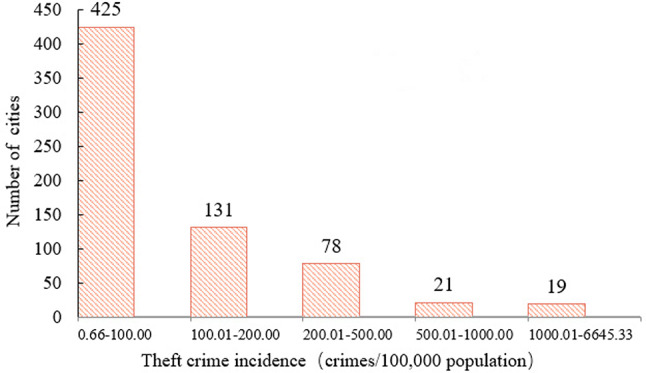
Number of cities with varying levels of theft crimes.

To visually demonstrate the uneven regional distribution of theft crime numbers in China, we utilized ArcGIS to visualize the spatial pattern of theft crime occurrences (see Fig. 2). Overall, the number of theft crimes in China exhibits a decreasing trend from the eastern, central, to western regions. Theft crimes are primarily concentrated in the Yangtze River Delta, Beijing–Tianjin–Hebei region, Pearl River Delta, and other economically developed cities or provincial capitals. The results reveal a significant imbalance and substantial regional disparities in the occurrence of theft crimes across geographical spaces in China, suggesting a need for heightened attention to the key cities where theft crimes frequently occur.

Fig. 2.

Spatial patterns of the number of theft crimes in cities in China.

In the spatial autocorrelation analysis spanning 674 cities in China, a Moran’s I index of 0.201095 was determined. This figure underscores a pronounced positive spatial autocorrelation regarding theft crime incidents, suggesting that cities with similar crime rates are geographically clustered. The z-score, at 3.734666, not only surpasses the critical threshold of 2.58 for the 0.01 significance level but also affirms the clustering pattern’s statistical significance, with a p-value as low as 0.000188. This near-certitude level of significance indicates that the observed clustering is not a random occurrence. The Table 2 suggest that theft crime distribution within the study area follows a pattern of aggregation rather than being randomly dispersed, with spatial autocorrelation potentially linking crime rates in neighboring cities through unspecified underlying factors. Given the Bayesian model’s adeptness at capturing inter-regional interdependencies and its flexibility, this study adopts a Bayesian approach to delve into the spatial distribution patterns of theft crime.

Table 2.

shows the results of spatial autocorrelation analysis.

Category	Moran’s I	Z score	P Value
Average Theft Cases	0.201	3.735	0.000

Bayesian model-based fitting of crime in Chinese cities

This study employs a Bayesian modeling approach to conduct an in-depth fitting analysis of theft crime occurrences by selecting four key indicators: population size (permanent resident population), economic size (total GDP), geographical size (built-up area), and functional size (total number of POI). Figure 3 presents the spatial patterns of theft crimes as presented by the four fitting indicators, revealing the multi-faceted and complex factors influencing the distribution of theft crimes.

Fig. 3.

Spatial patterns of theft crimes presented by different indicators fitting.

By using the Bayesian modeling method to fit theft crime occurrences, the Bayesian fitting curves for different indicators are shown in Fig. 4, and the DIC values are presented in Table 3. As shown in Table 3, the DIC value for the total number of POIs is the smallest (5427.86), while the largest DIC value belongs to the built-up area (5462.27). In Bayesian model selection a smaller DIC value with a difference above 5 between indicators indicates a better fit of that indicator for the model. Therefore, among the four indicators, the total number of POIs exhibits the best fit for modeling urban crime, while the built-up area has a relatively poorer fit. In addition, the difference in DIC values between the total number of POIs and the other three indicators is substantial, with the maximum difference being 34.41 and the minimum being 17.53, suggesting a markedly pronounced difference in the fitting effectiveness among the indicators. The significant difference in DIC values between the total number of POIs and built-up area underscores the distinct effects of the two indicators in fitting crime. Conversely, the small DIC difference (i.e., below 5) between the permanent resident population and GDP implies that the two indicators have similar effectiveness in describing or predicting crime.

Fig. 4.

Bayesian curves fitted for different indicators.

Table 3.

DIC values for fitting crime with different indicators.

Indicator	Permanent Resident Population	GDP	Built-up Area	Total Number of POIs
DIC Value	5445.39	5449.53	5462.27	5427.86

POI, as an integral part of geospatial data, often reflects an area’s daily activity level, commercial prosperity, and population concentration. These factors are closely related to criminal activities. For example, regions with frequent commercial activities, owing to the density of people and logistics, tend to be considerably prone to theft, robbery, and other criminal behaviors. In addition, areas with a concentration of entertainment, dining, and other POIs may experience markedly prominent public security issues at night owing to increased foot traffic. By contrast, permanent resident population and GDP, as static indicators describing basic regional characteristics, generally exhibit smooth changes and minimally significant fluctuations in the short term. This stability may lead to less direct correlations with crime rates compared with POIs. However, this case does not mean they are unrelated to crime. The density of the permanent resident population and the region’s economic development level are crucial factors influencing crime rates. They may indirectly impact crime rates through a series of intermediary variables, such as social structure and cultural habits. The relationship between construction land, a manifestation of urbanization, and crime is considerably complex. On the one hand, rapid urban expansion may lead to lags in urban planning and public security management, thereby creating opportunities for criminal activities. On the other hand, the increase in construction land may also result in numerous job opportunities and high incomes for residents, which can relatively help reduce crime rates. Therefore, the unsatisfactory fitting effect of construction land and crime may reflect this complex relationship.

As shown in Table 3, there are differences in DIC values among different indicators when fitting crime data, with the lowest DIC value for the total number of POIs indicating a strong correlation with crime. To delve deeper into the relationship between POI and crime, the POI classification was further refined, resulting in separate Bayesian fitting curves for the number of crimes against different subcategories of POI (Fig. 5). In addition, the DIC values for fitting crimes with various POI indicators are presented in Table 4. This study conducts a detailed fitting study focusing on four dimensions: residential, commercial, public service, and corporate and enterprise POIs.

Fig. 5.

Bayesian fitting curves for different types of POIs.

Table 4.

DIC values for fitting crime with different types of POI indicators.

Indicator	Residential POIs	Commercial POIs	Public service POIs	Corporate and enterprise POIs
DIC value	5441.47	5429.48	5428.38	5434.19

Table 4 shows that public service POIs (DIC value of 5428.38) and commercial POIs (DIC value of 5429.48) have relatively lower DIC values, indicating better fitting effects with crime. The small difference of 1.1 between their DIC values suggests that public service and commercial POIs have similar effectiveness in fitting crime data. Residential POIs have the highest DIC value, with a difference of 13.09 from the best-fitting public service POIs, indicating that residential POIs have a relatively poorer fitting effect among the four indicators.

Residential POIs reveal the characteristics and density of residential areas, whereas commercial POIs map the hotspots of economic activities and consumer behaviors. Public service POIs embody the coverage of urban infrastructure and public services, and corporate and enterprise POIs represent the heart of urban economic activities. By analyzing the correlation between these different types of POIs and theft crime data, we can precisely depict the spatial pattern of theft crimes in various functional areas, revealing the underlying socioeconomic drivers and geographical factors behind them.

Discussion

In the current academic and practical fields, the fitting study of the total number of theft crimes generally focuses on traditional macro-indicators, such as population size, economic size, and land use size. These indicators have played a crucial role in revealing the socioeconomic background of criminal phenomena. Nevertheless, with the acceleration of urbanization and the increasing complexity of urban functions, relying solely on these traditional indicators has become insufficient to fully explore the underlying causes and spatial distribution characteristics of theft crimes. Given this situation, this study focuses on the functional size of cities, particularly through finely classified POI data, to delve into the intrinsic relationship between theft crimes and urban functional layouts. The functional size of a city, as an essential indicator measuring the diversity, vitality, and convenience of residents’ lives, encompasses various POIs, such as residential, commercial, public service, and corporate enterprises. These POIs reflect the complexity and diversity of urban spatial structures and also profoundly influence the occurrence and distribution of theft crimes.

Commercial POIs, as crucial indicators reflecting regional commercial activities and human traffic, often have a direct correlation with the frequency of criminal acts. These areas attract numerous customers and employees but also potential criminals, leading to frequent occurrences of theft, robbery, and other commercial-related crimes. Consequently, the fitting effect between commercial POIs and crimes is relatively significant, providing a solid basis for predicting and analyzing the law and order situation in commercial areas. Meanwhile, public service POIs, including parks, libraries, and hospitals, are indispensable components of residents’ daily lives. The completeness of these facilities often reflects the quality of life for residents and the level of social services and security. The good fitting effect between public service POIs and crimes may be attributed to the relatively better law and order conditions in these areas, resulting in lower crime rates and providing a safe and comfortable living environment for residents.

By contrast, residential POIs, representing the residential population and housing distribution in an area, exhibit a relatively weaker fitting effect with crimes. The primary reason is that residential POIs do not directly reflect crime inducements but are considerably intertwined with other social and economic factors that collectively influence crime risks. To accurately predict crime risks in residential areas, a combination of relevant factors must be considered. For corporate enterprise POIs, involving office spaces and industrial areas, they experience dense human traffic during the day but may be relatively quiet at night. Therefore, the fitting effect between corporate enterprise POIs and crimes is influenced by time and space, showing certain fluctuations. In some industrial areas, owing to poor management or inadequate security measures, there may be security issues, while in other strictly managed areas, crime rates may be relatively low. This case necessitates a markedly detailed and in-depth analysis of the relationship between corporate enterprise POIs and crimes.

In the fitting analysis of Bayesian models, Points of Interest (POIs) related to commerce and public services typically exhibit lower Deviance Information Criterion (DIC) values and superior model fit compared to residential and corporate POIs. This correlation is fundamentally attributed to the higher association with risk factors for theft crimes inherent in commercial and public service POIs. These POIs are often located in densely populated areas, such as shopping centers, restaurants, parks, libraries, and hospitals, which naturally increase the number of potential targets for crime and provide more opportunities for criminal activities. Moreover, the extended duration of activities in these areas, especially during sparsely populated nighttime hours, can inadvertently create conditions conducive to criminal behavior. The frequent display of wealth and valuables in commercial and public service venues may attract the attention of theft criminals. Although these areas may be equipped with more comprehensive surveillance systems, the existence of surveillance blind spots and security vulnerabilities can still be exploited by criminals.

In contrast, residential and corporate POI areas, characterized by lower foot traffic, stronger community surveillance, and stricter security measures, have a relatively lower association with theft crimes. Consequently, their fit in Bayesian models is not as pronounced as that of commercial and public service POIs. This finding suggests that policymakers and law enforcement agencies should place special emphasis on crime prevention efforts in areas with commercial and public service POIs to effectively reduce the incidence of theft crimes.

POI data offers a multidimensional perspective for crime mapping and spatial analysis, enabling a detailed portrayal of the geographical distribution of commercial activities, service facilities, and social interaction points. It reveals the socio-economic background and influencing factors of crime. Especially in areas with high incidence of theft crimes, POI data can significantly improve the accuracy of identifying crime hotspots, assisting law enforcement agencies in optimizing resource allocation and patrol strategies. Analyzing POI data with timestamps can also uncover the temporal patterns of criminal activities, enhancing the understanding of the spatiotemporal distribution of crime. Combined with machine learning, crime events can be predicted, providing timely warnings for law enforcement departments¹⁶. When integrated with other statistical data, POI data allows for a more accurate assessment of crime risks in specific areas, aiding in decision-making. Cross-departmental data integration platforms facilitate collaboration and enhance analysis efficiency. A regular evaluation mechanism ensures the continuous optimization of POI data applications, aiding in a deeper understanding of crime distribution and trend prediction, and providing data support for formulating preventive measures to jointly build safer cities.

Through a Bayesian model’s deep fitting analysis of theft crime data from 674 cities in China, we provide a novel perspective and pathway for studying urban theft crimes. In particular, the introduction of functional size-related indicators, such as POIs, presents a fresh perspective for delving into the complex relationship between theft crimes and urban spatial structures. This innovative practice coincides with Cichosz’ research on using POI data to predict urban crime interests, thereby demonstrating the immense potential and unique value of big data and spatial analysis in criminological studies¹⁶. To effectively prevent theft crimes in the future, we should focus on the following strategies. First, for urban areas with dense functional activities, a comprehensive, efficient, and intelligent security prevention and control system from a macro-strategic perspective must be established, thereby significantly strengthening the prevention and control of theft crimes. Second, given the significant attractiveness and fitting effect of commercial and public service POIs on theft crimes, these areas tend to be hotspots for theft crimes. To effectively address this issue, substantially precise and detailed prevention and control measures need to be adopted, delving into the urban fabric and focusing on areas with high concentrations of commercial and public service POIs to effectively curb the occurrence of theft crimes.

To effectively deter theft and enhance urban security, policymakers can adopt strategies such as bolstering police presence and refining surveillance in high-theft areas like commercial zones and public service spots, employing smart monitoring to prevent and respond to criminal activities. Additionally, intensifying night-time lighting through additional streetlights or brighter illumination and implementing environmental design interventions—like natural barriers with greenery and physical obstacles—to restrict unauthorized access can augment safety. Decentralizing commercial and public service facilities to disperse crowds and mitigate crime risks, along with promoting the development of integrated urban complexes that combine residential, occupational, and recreational spaces, can minimize necessary travel and reduce opportunities for crime.

Note that although this study has made significant progress in applying the Bayesian model to fit and analyze theft crime data from 674 cities in China, we must acknowledge its limitations as well. In particular, the types of indicators used in the study are relatively limited and fail to comprehensively cover all factors that may influence theft crimes. In addition, the period of the study is insufficient to fully reveal the comprehensive picture of the long-term evolution of theft crimes. Looking ahead, county-level data can be included in the statistical data to expand the scope of case areas. By increasing the diversity and representativeness of samples, we will be able to more comprehensively summarize the laws and characteristics of theft crimes, providing strong support for formulating more precise and effective public security policies. Furthermore, continuously optimizing research methods and introducing significantly advanced statistical analysis tools and technical means will be important avenues for improving research quality and deepening research levels.

Conclusion

With the acceleration of urbanization, the spatial distribution pattern of theft crimes has become increasingly intricate. The Bayesian model, with its capabilities in handling small samples, addressing overdispersion, and spatial autocorrelation, provides a powerful tool to gain a comprehensive insight into the spatial distribution of theft crimes. Its comprehensiveness and flexibility have demonstrated significant advantages in research, warranting widespread promotion and application. This study focuses on theft crime data from 674 cities in China and utilizes the Bayesian model to fit the data, revealing that urban functional sizes, particularly urban functional areas represented by POIs, perform exceptionally well in predicting and fitting theft crimes. In particular, public service and commercial POIs exhibit the most notable fitting effects, indicating a close relationship between urban functional layouts and theft crime risks. Furthermore, this study reveals a trend of declining theft crime rates geographically from the eastern to the central and western regions of China. in particular, high-incidence areas of theft crimes are primarily concentrated in economically prosperous regions, such as the Yangtze River Delta, Beijing–Tianjin–Hebei, and Pearl River Delta, as well as other economically developed cities or provincial capitals.

Electronic Supplementary Material

Below is the link to the electronic supplementary material.

Author contributions

Author contributionsHaolei Zheng：Analyzed and interpreted the data; Writing-original draft; Validation.Daqian Liu：Methodology; Theoretical analysis; Writing-original draft.Yang Wang：Conceptualization; Writing—review and editing; Visualization; Project management.Xiaoli Yue：Data analysis; Materials.

Data availability

All data generated or analysed during this study are included in this published article [and its supplementary information files].

Declarations

Competing interests

The authors declare no competing interests.

Ethical approval

This article does not contain any studies with human participants performed by any of the authors.

Informed consent

This article does not contain any studies with human participants performed by any of the authors.

References

- 1.Eilstrup-Sangiovanni, M. & Hofmann, S. C. Of the contemporary global order, crisis, and change. J. Eur. Public. Policy. 27, 1077–1089 (2020). [Google Scholar]
- 2.Kerry, R., Goovaerts, P., Haining, R. P. & Ceccato, V. Applying geostatistical analysis to crime data: Car-related thefts in the Baltic states. Geogr. Anal.42, 53–77 (2010). [DOI] [PMC free article] [PubMed] [Google Scholar]
- 3.Lee, B., Lee, J. & Hoover, L. Neighborhood characteristics and auto theft: An empirical research from the social disorganization perspective. Secur. J.29, 400–408 (2016). [Google Scholar]
- 4.Silva, P. & Li, L. Urban Crime occurrences in association with built environment characteristics: An African case with implications for urban design. Sustainability. 12, 3056 (2020). [Google Scholar]
- 5.Sypion-Dutkowska, N., Lan, M., Dutkowski, M. & Williams, V. Different ways ambient and immobile population distributions influence urban crime patterns. IJGI. 11, 581 (2022). [Google Scholar]
- 6.Hipp, J. R. & Kane, K. Cities and the larger context: What explains changing levels of crime? J. Criminal Justice. 49, 32–44 (2017). [Google Scholar]
- 7.Caminha, C. et al. Human mobility in large cities as a proxy for crime. PLoS One. 12, e0171609 (2017). [DOI] [PMC free article] [PubMed] [Google Scholar]
- 8.He, L. et al. Ambient population and larceny-theft: A spatial analysis using mobile phone data. ISPRS Int. J. Geo-Inf9, 342 (2020).
- 9.Rosenfeld, R., Vogel, M. & McCuddy, T. Crime and inflation. S Cities J. Quant. Criminol.35, 195–210 (2019). [Google Scholar]
- 10.Hegerty, S. W. Crime, housing tenure, and economic deprivation: Evidence from Milwaukee, Wisconsin. J. Urban Affairs. 39, 1103–1121 (2017). [Google Scholar]
- 11.Kondo, M., Hohl, B., Han, S. & Branas, C. Effects of greening and community reuse of vacant lots on crime. Urban Stud.53, 3279–3295 (2016). [DOI] [PMC free article] [PubMed] [Google Scholar]
- 12.Ioannidis, I., Haining, R. P., Ceccato, V. & Nascetti, A. Using remote sensing data to derive built-form indexes to analyze the geography of residential burglary and street thefts. Cartogr. Geogr. Inf. Sci.10.1080/15230406.2023.2296598 (2024). [Google Scholar]
- 13.Li, N. & Kim, Y. A. Subway Station and Neighborhood Crime: An egohood analysis using subway ridership and crime data in New York City. Crime. Delinq69, 2303–2328 (2023).
- 14.Gaigné, C. & Zenou, Y. Agglomeration, city size and crime. Eur. Econ. Rev.80, 62–82 (2015). [Google Scholar]
- 15.Sohn, D. W. Residential crimes and neighbourhood built environment: Assessing the effectiveness of crime prevention through environmental design (CPTED). Cities. 52, 86–93 (2016). [Google Scholar]
- 16.Cichosz, P. Urban crime risk prediction using point of interest data. ISPRS Int. J. Geo-Inf. 9, 459 (2020). [Google Scholar]
- 17.Kim, S. & Lee, S. Nonlinear relationships and interaction effects of an urban environment on crime incidence: Application of urban big data and an interpretable machine learning method. Sust Cities Soc.91, 104419 (2023). [Google Scholar]
- 18.Kadar, C. & Pletikosa, I. Mining large-scale human mobility data for long-term crime prediction. EPJ Data Sci.7, 26 (2018). [Google Scholar]
- 19.Chung, J. & Kim, H. Crime risk maps: A multivariate spatial analysis of crime data. Geogr. Anal.51, 475–499 (2019). [Google Scholar]
- 20.Tseloni, A. & Pease, K. Population inequality: The case of repeat crime victimization. Int. Rev. Victimology. 12, 75–90 (2005). [Google Scholar]
- 21.Best, N., Richardson, S. & Thomson, A. A comparison of Bayesian spatial models for disease mapping. Stat. Methods Med. Res.14, 35–59 (2005). [DOI] [PubMed] [Google Scholar]
- 22.Osei, F. B., Duker, A. A. & Stein, A. Bayesian structured additive regression modeling of epidemic data: Application to cholera. BMC Med. Res. Methodol.12, 1–11 (2012). [DOI] [PMC free article] [PubMed] [Google Scholar]
- 23.Wang, Y., Chen, X. & Xue, F. A. Review of Bayesian spatiotemporal models in spatial epidemiology. ISPRS Int. J. Geo-Information. 13, 97 (2024). [Google Scholar]
- 24.Locke, D. H. et al. Vacant building removals associated with relative reductions in violent and property crimes in Baltimore, MD 2014–2019. J. Urban Health. 100, 666–675 (2023). [DOI] [PMC free article] [PubMed] [Google Scholar]
- 25.De Nadai, M., Xu, Y., Letouz, E., Gonzalez, M. C. & Lepri, B. Socio-economic, built environment, and mobility conditions associated with crime: A study of multiple cities. Sci. Rep.10, 13871 (2020). [DOI] [PMC free article] [PubMed] [Google Scholar]
- 26.Liu, H. & Zhu, X. Joint modeling of multiple crimes: A Bayesian spatial approach. ISPRS Int. J. Geo-Inf. 6, 16 (2017). [Google Scholar]
- 27.Matthews, S. A., Yang, T. C., Hayslett-McCall, K. L. & Ruback, R. B. Built environment and Property Crime in Seattle, 1998–2000: A Bayesian Analysis. Environ. Plan. A. 42, 1403–1420 (2010). [DOI] [PMC free article] [PubMed] [Google Scholar]
- 28.Shaw, C. R. & McKay, H. D. Juvenile Delinquency and Urban Areas xxxii, 451 (University of Chicago Press, 1942).
- 29.Cohen, L. E. & Felson, M. Social change and crime rate trends: A routine activity approach. Am. Sociol. Rev.44, 588–608 (1979). [Google Scholar]
- 30.Liu, L., Li, C., Xiao, L. & Song, G. Explaining theft using offenders’ activity space inferred from residents’ mobile phone data. ISPRS Int. J. Geo-Inf. 13, 8 (2024). [Google Scholar]
- 31.Sypion-Dutkowska, N. & Leitner, M. Land use influencing the spatial distribution of urban crime: A case study of Szczecin. Pol. IJGI. 6, 74 (2017). [Google Scholar]
- 32.Cowen, C., Louderback, E. R. & Sen Roy, S. The role of land use and walkability in predicting crime patterns: A spatiotemporal analysis of Miami-Dade County neighborhoods, 2007–2015. Secur. J.32, 264–286 (2019). [Google Scholar]
- 33.Hipp, J. R. Spreading the Wealth: The effect of the distribution of income and race/ethnicity across households and neighborhoods on city crime trajectories*. Criminology. 49, 631–665 (2011). [Google Scholar]
- 34.Quick, M., Li, G. & Brunton-Smith, I. Crime-general and crime-specific spatial patterns: A multivariate spatial analysis of four crime types at the small-area scale. J. Criminal Justice. 58, 22–32 (2018). [Google Scholar]
- 35.Andresen, M. A. Testing for similarity in area-based spatial patterns: A nonparametric Monte Carlo approach. Appl. Geogr.29, 333–345 (2009). [Google Scholar]
- 36.Adeyemi, R. A., Mayaki, J., Zewotir, T. T. & Ramroop, S. Demography and Crime: A spatial analysis of geographical patterns and risk factors of crimes in Nigeria. Spat. Stat.41, 100485 (2021). [Google Scholar]
- 37.Hipp, J. R. & Roussell, A. Micro- and macro-environment population and the consequences for crime rates. Soc. Forces. 92, 563–595 (2013). [Google Scholar]
- 38.Xu, C., Chen, X., Chen, J. & Chen, D. Exploring the impact of floating population with different household registration on theft. ISPRS Int. J. Geo-Inf. 11, 443 (2022). [Google Scholar]
- 39.Metz, N. & Burdina, M. Neighbourhood income inequality and property crime. Urban Stud.55, 133–150 (2018). [Google Scholar]
- 40.Gatrell, A. C. Autocorrelation in spaces. Environ. Plan. A. 11, 507–516 (1979). [Google Scholar]
- 41.Liu, D., Song, W., Xiu, C. & Xu, J. Understanding the spatiotemporal pattern of crimes in Changchun, China: A Bayesian modeling approach. Sustainability. 13, 10500 (2021). [Google Scholar]
- 42.Hua, P. & Zhao, X. A. Review of Bayesian model averaging. In Data Processing and Quantitative Economy Modeling (eds. Zhu, K. L. & Zhang, H.) 32-+ (Aussino Acad Publ House, 2010).
- 43.Alexander, N. Bayesian disease mapping: Hierarchical modeling in spatial epidemiology. J. Royal Stat. Soc. Ser. A: Stat. Soc.174, 512–513 (2011). [Google Scholar]
- 44.Besag, J., York, J. & Mollié, A. Bayesian image restoration, with two applications in spatial statistics. Ann. Inst. Stat. Math.43, 1–20 (1991). [Google Scholar]
- 45.Blangiardo, M., Cameletti, M., Baio, G. & Rue, H. Spatial and spatio-temporal models with R-INLA. Spat. Spatio-temporal Epidemiol.7, 39–55 (2013). [DOI] [PubMed] [Google Scholar]
- 46.Bakka, H. et al. Spatial modeling with R-INLA: A review. WIRE Comput. Stat.10, e1443 (2018). [Google Scholar]
- 47.Shriner, D. & Yi, N. Deviance information criterion (DIC) in Bayesian multiple QTL mapping. Comput. Stat. Data Anal.53, 1850–1860 (2009). [DOI] [PMC free article] [PubMed] [Google Scholar]
- 48.Dogan, O. Integrated deviance information criterion for spatial autoregressive models with heteroskedasticity. Spat. Stat.61, 100842 (2024). [Google Scholar]
- 49.Spiegelhalter, D. J., Best, N. G., Carlin, B. P. & Van Der Linde, A. Bayesian measures of model complexity and fit. J. Royal Stat. Society: Ser. B (Statistical Methodology). 64, 583–639 (2002). [Google Scholar]
- 50.Law, J., Quick, M. & Chan, P. Bayesian spatio-temporal modeling for analysing local patterns of crime over time at the small-area level. J. Quant. Criminol.30, 57–78 (2014). [Google Scholar]
Associated Data
This section collects any data citations, data availability statements, or supplementary materials included in this article.
Supplementary Materials
Data Availability Statement