Investigation of linear and microscopic nonlinear optical responses of 1-indanone compounds in different environments based on polarity models

Abstract

Molecular spectroscopic and nonlinear features can indicate positive changes by solvent molecules. In this work, DFT and spectroscopic techniques were used to study the polarity effects of different solvent environments. Polarity-based models were used for studying solvent induced interactions on the optical features of new groups of biomolecules. Despite the significant contribution of general effects on the molecular absorption spectra, there is considerable competition between general and specific environmental effects on the molecular emission properties. Under this condition, strong hydrogen bonds tend to increase molecular nonlinear responses. The same results were observed for the low order (first and second order) nonlinearity of biomolecules. Therefore, the studies on the environment effects on the biomolecules’ first order nonlinearity can give valuable information about higher-order optical responses. Moreover, 1-Indanone compounds with high nonlinearity can be considered as an effective element in designing optical devices.

Supplementary Information

The online version contains supplementary material available at 10.1038/s41598-024-78194-9.

Introduction

1-Indanone compounds with unique structures and biologically active groups in their chemical structures are important in pharmacology. They are involved in biologically important activities because of their anti-inflammatory¹, anti-cholinergic², antimalarial³, anti-microbial⁴, anticancer⁵, analgesic⁶, and dopaminergic⁷ properties. This moiety is usually found in some natural compounds and is used as an intermediate in the synthesis process of various biological molecules with wide application in the treatment of diseases. Among various diseases, today, Alzheimer’s is a great threat to human health by increasing the elderly population. In this case, drugs with 1-indanone moiety and enzyme inhibitor characteristics can play a main role in treating Alzheimer’s disease^8–10.

Moreover, important biological activities of indanone compounds may be modified by their surrounding environment properties. The study of the various biological characteristics of molecules is generally done in the solution. Under this circumstance, interactions between the selected molecules and their environmental molecules are a significant issue in their function. In this case, studies on possible molecular interactions with different contributions are significant in explaining various phenomena.

Molecular interactions are separated into two categories: general and specific interactions. The first groups are directional, induction, and dispersion forces that cannot be saturated completely. The second group comprises hydrogen bonds, and electron-pair donor–acceptor forces which can be saturated and lead to stoichiometric molecular compounds^11–13. Studies have indicated that solvents can modify the intensity, and position of absorption bands studied molecules. Solvent effects are usually described using environment polarity scales and solvatochromic parameters^11–16. However, single solvent polarity parameters such as solvent orientation polarizability parameters may be used to approximate solvent effects. The Kamlet-Abboud-Taft formulation (Eq. 1) with multi-parameter polarity scales is a good model for studying environmental effects¹¹.

1

In Eq. 1, a, b, and c are regression coefficients that display the strength of various polarity effects. In the Kamlet-Abboud-Taft model, A, B, and C are indicated by α, β, and π*, respectively. α, and β explain hydrogen bonds^17,18, and π* is solvent dipolarity/polarizability ability¹⁹. y₀ is also obtained from the analysis. To separate general environment effects, the Catalan model can be considered as a proper selection. In this case, A, B, and C are indicated by SA, SB, and SPP. In this formalism, SA, SB, and SPP are selected environment acidity, basicity, and dipolarity/polarizability, respectively^20,21. The last solvent polarity parameter can be divided into SP and SdP parameters.

Moreover, light-mater interactions at the molecular level in the linear and nonlinear optical domains can limit the activity of biologically important molecules in the solution state. The studies on the various optical responses of understudy molecules will provide essential information about their function in different processes.

In this experimental research, the effects of environment polarity on the optical behavior of some 1-Indanone compounds were investigated in linear and nonlinear optics domains. In this case, the spectroscopic technique and density functional theory (DFT) theoretical method were used for studying the optical properties of understudy samples in various environments with different features. In addition, the obtained results from a simple experimental method were used to quantitatively detect the effects of polarity-sensitive features of some biologically important molecules. It is expected that results can give a simple way to improve the nonlinearity of biomolecules. Moreover, the data will give interesting results for increasing the application of 1-Indanone compounds in optics and photonics.

Experimental section

Material

In this work, 1-Indanone compounds with different substituents, as shown in Fig. 1, were synthesized according to our previous work^22,23. Detailed information about synthesis materials is available in references 20 and 21. The selected solvent environments with different polarities were bought from Merck¹¹. The polarity parameters of these solvents are summarized in Table 1.

Fig. 1.

Chemical structure and name of (a) sample I, (b) sample II, (c) sample III, and (d) sample IV.

Table 1.

Polarity parameters of selected solvents. (α: Solvent hydrogen bond donor ability, β: Solvent hydrogen bond acceptor ability, π*: Solvent dipolarity/polarizability ability, SA: Solvent acidity, SB: Solvent basicity, SP: Solvent polarizability, and SdP: Solvent dipolarity.)

Solvent	α	β	π*	SP	SdP	SA	SB
DMSO	0.00	0.76	1.00	0.83	1	0.072	0.647
DMF	0.00	0.69	0.88	0.759	0.977	0.031	0.613
Methanol	0.98	0.66	0.60	0.608	0.904	0.605	0.545
Ethanol	0.86	0.75	0.54	0.633	0.783	0.4	0.658
Acetone	0.08	0.48	0.62	0.651	0.907	0.00	0.475
2-propanol	0.76	0.84	0.48	0.633	0.808	0.283	0.83
1-Butanol	0.84	0.84	0.47	0.674	0.655	0.341	0.809
1-Hexanol	0.67	0.94	0.40	0.698	0.552	0.315	0.879
Dichloromethane	0.13	0.1	0.73	0.761	0.769	0.04	0.178
Diethyl ether	0.00	0.47	0.24	0.617	0.385	0.00	0.562
Benzene	0.00	0.1	0.59	0.793	0.27	0.00	0.124
1,4-Dioxane	0.00	0.37	0.49	0.737	0.312	0.00	0.444
Cyclohexane	0.00	0.00	0.00	0.683	0.00	0.00	0.073

Spectroscopic techniques

In this experimental work, first, prepared solutions with special concentration (0.000005 M) were poured into the spectroscopic cell. Then, absorption and fluorescence spectra of 1-Indanone compounds at room temperature were recorded by a double-beam Shimadzu (UV-1800) spectrometer and Jasco spectrofluorometer (FP-6200), respectively. In this experiment, the accuracy of the spectrometer was 0.1 nm. Moreover, a quartz cell (1 cm thickness) was used for spectroscopy.

Theoretical methods

In this section, first, the optimization of the structure of 1-Indanone compounds was done using the DFT approach. Then, the CAM-B3LYP hybrid function was selected²⁴ and 6-311 + G(d, p) basis sets were applied for carbon, hydrogen, oxygen, and nitrogen atoms, and the DGDZVP basis was selected for the bromine atom^25,26. Also, the basis set superposition error (BSSE) was considered for the calculations²⁷. The solvation model based on the density (SMD) method was used to investigate solvent media²⁸. The required solvent properties for SMD calculations including: refractive index at 293 K (n), Abraham’s hydrogen bond acidity (α), and basicity (β), macroscopic surface tension at liquid-air interface at 298 K (γ), and dielectric constant at 298 K (ε), are listed in Table 2 and were obtained from Minnesota solvent descriptor database²⁹. The optimized structures of the molecules are accessible in Fig. 2. These optimized structures were selected to determine their vertical electronic excitations by the time-dependent density functional theory (TDDFT) method³⁰. The results for TDDFT calculations are given in Table 3. Finally, the Onsager radii of the molecules were calculated³¹. The calculated Onsager radii for the molecules in different solvent media are listed in Table 3. It should be noted that the NWchem quantum chemistry program was used for all calculations³².

Table 2.

Refractive index at 293 K (n), Abraham’s hydrogen bond acidity (α), Abraham’s hydrogen bond basicity (β), macroscopic surface tension at liquid-air interface at 298 K (γ), and dielectric constant at 298 K (ε), used for SMD calculations.

Solvent	n	α	β	γ	ε
DMSO	1.4783	0.00	0.88	61.78	46.826
DMF	1.4305	0.00	0.74	49.56	37.219
Methanol	1.3288	0.43	0.47	31.77	32.613
Ethanol	1.3611	0.37	0.48	31.62	24.852
Acetone	1.3588	0.04	0.49	33.77	20.493
2-propanol	1.3776	0.33	0.56	30.13	19.264
1-Butanol	1.3993	0.37	0.48	35.88	17.332
1-Hexanol	1.4178	0.37	0.48	37.15	12.510
Dichloromethane	1.4242	0.10	0.05	39.15	8.930
Diethyl ether	1.3526	0.00	0.41	23.96	4.240
Benzene	1.5011	0.00	0.14	40.62	2.271
1,4-Dioxane	1.4224	0.00	0.64	47.14	2.210
Cyclohexane	1.4266	0.00	0.00	35.48	2.016

Fig. 2.

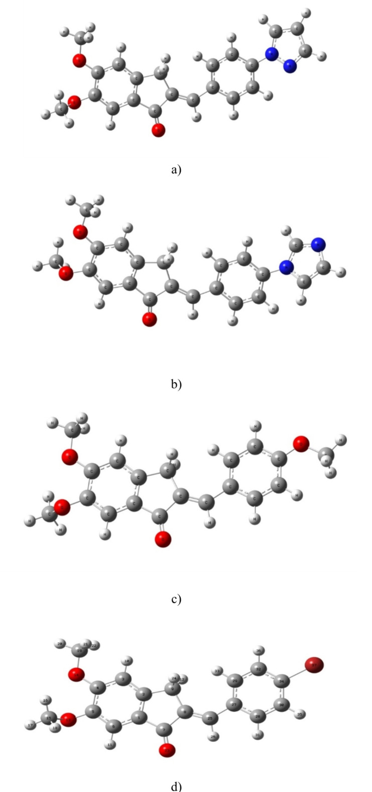
Optimized structure of (a) sample I, (b) sample II, (c) sample III, (d) sample IV.

Table 3.

DFT results of selected samples. (a₀: Onsager radii, and λ_max: maximum absorption wavelength)

Solvent	λmax (nm)	a0(Å)	λmax	a0(Å)
Sample I Sample II
DMSO	323.79	5.66	317.7	5.53
DMF	323.89	5.53	317.75	5.67
Methanol	331.20	5.53	324.8	5.53
Ethanol	330.05	5.50	323.63	5.70
Acetone	323.08	5.47	316.8	5.45
2-propanol	328.97	5.86	322.36	5.53
1-Butanol	330.20	5.56	323.61	5.55
1-Hexanol	329.83	5.72	323.09	5.69
Dichloromethane	324.06	5.53	317.36	5.53
Diethyl ether	320.16	5.27	313.16	5.49
Benzene	320.74	5.70	316.8	5.81
1,4-Dioxane	319.56	5.75	311.83	5.57
Cyclohexane	319.44	5.51	311.55	5.69
solvent
Sample III Sample IV
DMSO	324.77	5.58	311.97	5.28
DMF	324.87	5.4	312.06	5.04
Methanol	332.79	5.27	318.82	5.30
Ethanol	331.61	5.46	317.52	5.60
Acetone	323.84	5.44	311.29	5.20
2-propanol	330.5	5.59	316.59	5.47
1-Butanol	331.68	5.72	317.57	5.53
1-Hexanol	331.17	5.69	317.19	5.15
Dichloromethane	324.61	5.55	311.97	5.47
Diethyl ether	319.52	5.6	308.29	5.15
Benzene	318.81	5.44	308.11	5.25
1,4-Dioxane	317.49	5.43	307.09	5.30
Cyclohexane	317.03	5.38	306.82	5.40

Result and discussion

Linear optical properties of 1-Indanone compounds

In this section, to investigate the optical features of prepared solutions of biomolecules, first absorption and then fluorescence spectra were measured at (25 ± 0.1) °C. As shown in Figs. 3, 4, 5 and 6 and data in Table 4, the spectral properties of biomolecules depend on their surrounding the environment features. The effects of environment are usually detected using some important polarity scales. In this study, the concentration of solutions was low (5 × 10^− 6 M) that decrease the probability of aggregation process^33–35. 1-Indanon compounds can indicate different resonance structures in different solvents due to solute-solvent molecular that lead to observation of weak peaks. In this work, the main peak, which is more probable from the quantum point of view, has been investigated and analyzed.

Fig. 3.

(a) Absorption, (b) fluorescence spectra of sample I.

Fig. 4.

(a) Absorption, (b) fluorescence spectra of sample II.

Fig. 5.

(a) Absorption, (b) fluorescence spectra of sample III.

Fig. 6.

(a) Absorption, (b) fluorescence spectra of sample IV.

Table 4.

Maximum absorption and fluorescence of sample I, sample II, sample III, and sample IV.

Solvent name	λmax(Abs)(nm)	λmax(Flu)(nm)	λmax(Abs)(nm)	λmax(Flu)(nm)
Sample I Sample II
DMSO	348	492	341	483
DMF	348	496	339	484
Methanol	347	498	333	501
Ethanol	350	493	336	499
Acetone	350	503	355	488
2-propanol	350	488	336	493
1-Butanol	351	487	336	492
1-Hexanol	352	483	335	490
Dichloromethane	343	412	335	431
Diethyl ether	343	458	318	405
Benzene	349	434	334	414
1,4-Dioxane	343	409	332	410
Cyclohexane	364	444	363	442
solvent
Sample III Sample IV
DMSO	358	443	330	492
DMF	357	421	327	476
Methanol	361	474	328	502
Ethanol	362	466	330	496
Acetone	350	453	353	481
2-propanol	363	456	330	491
1-Butanol	363	457	330	490
1-Hexanol	362	456	330	488
Dichloromethane	354	432	326	431
Diethyl ether	347	404	317	408
Benzene	350	436	327	433
1,4-Dioxane	346	433	312	410
Cyclohexane	359	437	----	----

For precise investigation, the maximum wavelength of absorption and fluorescence spectra was plotted based on selected solvents’ dielectric constant. According to Fig. 7, sample solutions indicate positive solvatochromism behavior as the dielectric constant of the solutions increases. The different spectral shifts in sample solutions are correlated to different substituents. Compared to other samples, the maximum red shifts are obtained in sample IV with bromobenzene. These results are consistent with DFT results. The differences can be understood by considering various scientific approximations (Table 3). It is noticeable that some differences can be seen between DFT results in Table 3, and the experimental data of Table 4 for samples I and II, in such a way that DFT results predict a decrease in λ_max from DMF to cyclohexane for samples I, and II. However, experimental values of λ_max demonstrate more fluctuations with polarity of the solvent and show the longest λ_max for cyclohexane solvent for samples I, and II. The main reason for these differences arises from the implicit inclusion of the solvent as a continuous dielectric environment for DFT calculations. At these circumstances, some specific interactions between the solvent and the solute cannot be considered, exactly. Especially, when the charge transfer between two parts of the solute molecule strongly depends on some dihedral angles between the related fragments of the solute molecule, the differences between DFT results and experimental data becomes more important³⁶. By consideration of the optimized structures of samples I, and II, it can be observed that the dihedral angle between 5-membered C₃N₂ ring and its vicinal phenyl ring can play an important role in the charge transfer for these molecules. Due to the existence of two electronegative N atoms in the C₃N₂ ring, its interactions with small and more polar solvent molecules can be significant which may lead to torsion of the mentioned dihedral angle and can reduce the probability of charge transfer between C₃N₂ ring and its vicinal phenyl group. Hence one can expect that molecules I, and II may be more flat in cyclohexane solvent due to its high steric hindrance and non-polar nature which can make the charge transfer between C₃N₂ ring and its vicinal phenyl group, easier and give the highest for cyclohexane solvent. Whereas, DFT calculations predict similar values for the mentioned dihedral angle, see Table S1 of Supporting Information. The other source of the differences can be related to the problematic performance of TDDFT for the lowest π→π* transitions in the molecules containing heterocyclic fragments³⁶. Despite of the mentioned problems, the reasonable agreement between TDDFT results with acceptable computational cost and experimental data makes it the most appropriate and applicable theoretical method for vertical excitations.

Fig. 7.

Variation of (a) maximum absorption, (b) maximum fluorescence, and (c) Stokes shift of sample I, sample II, sample III, and sample IV as a function of dielectric constant of selected solvents.

Moreover, the bathochromic shifts in the fluorescence process are more significant than the absorption process. In contrast to the absorption phenomenon, fluorescence appears from a relaxed state. Indeed, this optical process is a relatively slow process in comparison to the absorption phenomenon. Solvent molecules in the excited state have time to reorient around the understudy molecule, leading to the emission phenomenon from a relaxed state. In this case, the differences between the maximum wavelength of absorption and fluorescence spectra lead to Stokes shift. According to Fig. 7, the Stokes shifts are increased by an increment of the solvent single polarity factor because of the reorientation of molecules. Under these conditions, the molecular interactions can modify solute molecules’ electronic structures and resonance forms. Hence, Lippert Mataga’s solvent model that describes the general environment effects can be applicable for calculating solute molecules’ ground and first-order excited state dipole moments in different solvents. According to Eq. 2, a linear behavior between Stokes shift data (υ_a-υ_f) and Lippert Mataga’s polarity (f_LM)³⁷ function is a simple way for calculating the changes between dipole moments of ground and first-order excited states.

In Eq. 2, b is constant. a, c, ε, n, h, and Δµ are also Onsager radius, light velocity in vacuum, used solvents’ dielectric constant, used solvents’ refractive index, Planck’s constant, and the changes between dipole moments, respectively.

2

The variation of Stokes shift values of 1-indanon compounds with different substituents based on orientation polarity function is indicated in Fig. 8. Using this figure, the differences between the dipole moments were calculated according to the data in Table 5, and Table 6. The obtained data indicate the possibility of charge transfer by exciting biomolecules in environments with different polarities. The different dipole moment values are due to active groups in the structure of solute molecules that lead to various interactions between solute and solvent molecules with different strengths. Therefore, the function of these compounds can be modified because of the presence of solvent molecules and various substituents in their chemical structures. According to our results, solute molecules with different chemical groups operate differently in solvent environments. These behaviors are related to different contributions of various molecular interactions. Although some polarity parameters such as dielectric constant can be considered for a qualitative investigation of solvent-induced general effects, they cannot fully explain the contribution of different molecular interactions. Hence, in the next section, some applicable models will be used.

Fig. 8.

Stokes shift changes of sample I, sample II, sample III, and sample IV based on Lippert Mataga’s polarity function.

Table 5.

The experimental results of sample I, and sample II in esu units. (Δµ: differences between ground and excited state dipole moments, f: oscillator strength, µ: transition dipole moment, α’: Linear polarizability, β’: first-order hyperpolarizability, and γ’: second order hyperpolarizability)

Solvent name	ΔµLP × 10− 18	f	µ × 10− 18	α’ × 10− 23	β’× 10− 29	γ’ × 10− 33
Sample I
DMSO	14.661	0.355	7.486	1.970	3.784	1.555
DMF	14.158	0.383	7.784	2.129	3.951	1.568
Methanol	14.158	0.438	8.311	2.421	4.478	1.772
Ethanol	14.043	0.454	8.492	2.549	4.718	1.868
Acetone	13.929	0.452	8.473	2.538	4.658	1.829
2-propanol	15.444	0.445	8.407	2.498	5.085	2.214
1-Butanol	14.274	0.440	8.379	2.489	4.696	1.895
1-Hexanol	14.894	0.390	7.894	2.215	4.373	1.847
Dichloromethane	14.158	0.066	3.227	0.360	0.659	0.258
Diethyl ether	13.172	0.217	5.814	1.171	1.992	0.725
Benzene	14.816	0.289	6.773	1.617	3.149	1.312
1,4-Dioxane	15.012	0.194	5.500	1.048	2.032	0.843
Cyclohexane	14.082	0.035	2.410	0.213	0.412	0.170
Sample II
DMSO	15.243	0.318	7.015	1.695	3.317	1.389
DMF	15.825	0.405	7.897	2.135	4.313	1.864
Methanol	15.243	0.485	8.568	2.469	4.719	1.930
Ethanol	15.951	0.501	8.741	2.593	5.233	2.260
Acetone	14.913	0.030	2.205	0.174	0.347	0.148
2-propanol	15.243	0.496	8.696	2.566	4.949	2.042
1-Butanol	15.326	0.486	8.613	2.517	4.881	2.025
1-Hexanol	15.909	0.433	8.114	2.228	4.470	1.919
Dichloromethane	15.243	0.335	7.142	1.726	3.319	1.365
Diethyl ether	15.078	0.325	6.857	1.510	2.726	1.053
Benzene	16.415	0.242	6.067	1.241	2.563	1.132
1,4-Dioxane	15.409	0.149	4.737	0.752	1.449	0.597
Cyclohexane	15.909	0.040	2.583	0.244	0.532	0.247

Table 6.

The experimental results of sample III, and sample IV in esu units.

Solvent name	ΔµLP × 10− 18	f	µ × 10− 18	α’ × 10− 23	β’× 10− 29	γ’ × 10− 33
Sample III
DMSO	17.181	0.298	6.959	1.751	4.055	2.009
DMF	16.356	0.310	7.088	1.812	3.983	1.874
Methanol	15.769	0.402	8.118	2.403	5.150	2.362
Ethanol	16.629	0.344	7.522	2.069	4.689	2.274
Acetone	16.538	0.068	3.303	0.385	0.840	0.392
2-propanol	17.227	0.390	8.021	2.359	5.554	2.798
1-Butanol	17.831	0.392	8.039	2.369	5.775	3.011
1-Hexanol	17.691	0.348	7.560	2.090	5.040	2.600
Dichloromethane	17.042	0.310	7.061	1.783	4.050	1.968
Diethyl ether	17.273	0.314	7.038	1.736	3.918	1.892
Benzene	16.538	0.300	6.909	1.687	3.678	1.715
1,4-Dioxane	16.492	0.188	5.441	1.034	2.223	1.022
Cyclohexane	16.265	0.036	2.445	0.216	0.476	0.224
Sample IV
DMSO	15.572	0.367	7.413	1.831	3.544	1.467
DMF	14.523	0.357	7.278	1.749	3.128	1.197
Methanol	15.661	0.543	8.997	2.682	5.187	2.146
Ethanol	17.009	0.525	8.873	2.624	5.546	2.508
Acetone	15.220	0.020	1.790	0.114	2.313	0.100
2-propanol	16.420	0.520	8.830	2.599	5.302	2.314
1-Butanol	16.691	0.522	8.842	2.606	5.404	2.398
1-Hexanol	15.001	0.488	8.549	2.436	4.540	1.810
Dichloromethane	16.420	0.397	7.663	1.933	3.897	1.681
Diethyl ether	15.001	0.267	6.199	1.230	2.203	0.844
Benzene	15.440	0.294	6.604	1.440	2.738	1.114
1,4-Dioxane	15.661	0.145	4.536	0.648	1.193	0.469
Cyclohexane	16.106	0.015	1.624	0.097	2.142	0.101

Linear properties and multi-parameter polarity models

In this work, the effect of three groups of solvents, polar aprotic (such as DMSO, and DMF), polar protic (such as alcohols), and nonpolar solvents, were studied. For precise investigation, multi-linear analysis was performed. In general, Kamlet-Abbod-Taft, and Catalan multi-parameters are applicable for studying the type and strength of interactions between various molecules. This analysis was performed in three steps as follows:

1. All selected solvents are considered in the analysis.

2. Some solvents may be deleted by paying attention to the values of statistical factor value (R²).

3. Multi-linear analysis of spectral results with Kamlet-Abbod-Taft and Catalan polarity scales was performed.

There is an excellent linear relation between the spectral data of sample solutions and solvent polarity parameters, as shown in Table 7, and Table 8. Furthermore, for a precise comparison of the behavior of various samples with each other, the contribution percentage of solvent polarity factors was calculated.

Table 7.

Regression fit to Kamlet-Abboud-Taft polarity scales for linear optical features of used samples with percentage contribution of various interactions. (a, b, and c: regression coefficients)

Multi-parameter scale	ν0(103cm−1)	a(103cm−1)	b(103cm−1)	c(103cm−1)	R 2
Sample I
Absorbance	27.632 ± 0.149	0.685 ± 0.194	-0.640 ± 0.242	1.775 ± 0.250	0.88
Fluorescence	23.281 ± 0.623	0.071 ± 0.817	-3.777 ± 1.068	0.182 ± 1.013	0.77
Stokes Shift	23.281 ± 0.623	0.071 ± 0.817	-3.777 ± 1.068	0.182 ± 1.013	0.86
Sample II
Absorbance	27.614 ± 0.438	1.643 ± 0.546	-0.216 ± 0.737	2.031 ± 0.715	0.78
Fluorescence	26.989 ± 0.920	-2.362 ± 0.798	-3.296 ± 1.116	-4.444 ± 1.263	0.86
Stokes Shift	4.640 ± 0.324	2.097 ± 0.424	2.903 ± 0.576	1.906 ± 0.545	0.95
Sample III
Absorbance	29.341 ± 0.210	-0.920 ± 0.182	-0.584 ± 0.254	-0.985 ± 0.288	0.90
Fluorescence	23.533 ± 0.440	-2.534 ± 0.583	0.852 ± 0.780	-0.900 ± 0.738	0.76
Stokes Shift	5.037 ± 0.377	2.064 ± 0.526	-1.840 ± 0.821	1.364 ± 0.722	0.70
Sample IV
Absorbance	32.444 ± 0.474	-0.874 ± 0.373	-0.742 ± 0.588	-1.563 ± 0.580	0.75
Fluorescence	26.527 ± 0.813	-2.348 ± 0.705	-2.584 ± 0.986	-4.462 ± 1.115	0.87
Stokes Shift	5.156 ± 0.399	1.866 ± 0.346	2.290 ± 0.484	2.997 ± 0.548	0.94
	Multi-parameter scale	Pα(%)	Pβ(%)	Pπ*(%)
	Sample I
	Absorbance	22	21	57
	Fluorescence	2	94	4
	Stokes Shift	30	4	66
	Sample II
	Absorbance	42	6	52
	Fluorescence	23	33	44
	Stokes Shift	30	42	28
	Sample III
	Absorbance	37	23	40
	Fluorescence	59	20	21
	Stokes Shift	39	35	26
	Sample IV
	Absorbance	28	23	49
	Fluorescence	25	28	47
	Stokes Shift	26	32	42

Table 8.

Regression fit to Catalan polarity scales for linear optical features of used samples with percentage contribution of various interactions.

Multi-parameter scale	ν0(cm− 1)	a(cm− 1)	b(cm− 1)	c(cm− 1)	d(cm− 1)	R 2
Sample I
Absorbance	30.439 ± 0.529	-1.118 ± 0.782	-0.157 ± 0.203	-0.569 ± 0.295	-1.056 ± 0.200	0.91
Fluorescence	24.493 ± 4.884	-0.108 ± 6.599	-2.384 ± 1.587	-1.746 ± 2.562	-3.511 ± 1.687	0.75
Stokes Shift	8.145 ± 3.250	-5.605 ± 4.483	2.893 ± 1.024	-0.250 ± 1.772	2.245 ± 1.308	0.78
Sample II
Absorbance	18.531 ± 3.136	13.985 ± 4.195	0.343 ± 0.681	3.776 ± 1.333	0.665 ± 0.863	0.72
Fluorescence	28.183 ± 3.031	-2.263 ± 3.986	-4.172 ± 0.998	-3.462 ± 1.556	-2.651 ± 1.220	0.88
Stokes Shift	4.000 ± 1.235	0.753 ± 1.704	2.145 ± 0.389	4.015 ± 0.673	2.638 ± 0.497	0.97
Sample III
Absorbance	30.881 ± 0.871	-2.437 ± 1.146	-0.461 ± 0.287	-1.830 ± 0.447	-0.790 ± 0.351	0.87
Fluorescence	-1.963 ± 2.747	0.698 ± 0.451	-4.532 ± 0.451	-4.532 ± 1.075	-0.166 ± 0.483	0.90
Stokes Shift	1.004 ± 1.789	6.236 ± 2.504	-1.020 ± 0.568	4.944 ± 0.982	-0.377 ± 0.609	0.79
Sample IV
Absorbance	33.514 ± 1.694	-1.296 ± 2.507	-1.050 ± 0.945	-1.050 ± 0.945	-0.999 ± 0.641	0.81
Fluorescence	29.153 ± 3.156	-4.799 ± 4.151	-3.453 ± 1.039	-4.138 ± 1.620	-1.994 ± 1.271	0.85
Stokes Shift	0.458 ± 1.283	7.780 ± 1.688	1.258 ± 0.422	4.870 ± 0.659	2.311 ± 0.516	0.95
	Multi-parameter scale	PSP(%)	PSdP(%)	PSA(%)	PSB(%)
	Sample I
	Absorbance	39	5	20	36
	Fluorescence	1	31	23	45
	Stokes Shift	51	26	2	21
	Sample II
	Absorbance	74	2	20	4
	Fluorescence	18	33	28	21
	Stokes Shift	8	22	42	28
	Sample III
	Absorbance	44	9	33	14
	Fluorescence	27	9	62	2
	Stokes Shift	50	8	39	3
	Sample IV
	Absorbance	27	31	20	22
	Fluorescence	33	24	29	14
	Stokes Shift	48	8	30	14

In biomolecules’ ground state, general interactions show a major role in the absorption characteristics of three selected samples. By optical excitation, general solvent effects still play the dominant role in sample II and sample IV. In sample I, the solvent environment hydrogen bond acceptor parameter with considerable contribution modifies the solute molecules’ linear optical behaviors. In sample III, hydrogen bond donor parameter has the dominant role. Stokes shifts also increase with the increase of the dominant media polarity factors.

In samples I, and IV, nonspecific polarity effects are significant in the Stokes shift values. In samples II, and III, specific solvent effects indicate significant roles. In this case, various substituents led to the detection of different types of molecular interactions with different contributions in the environments with different polarities.

The results show that solvent dipolarity/polarizability factor has considerable effects on the biomolecules’ optical linearity. Furthermore, the model presented by Catalan contains information about the dipolarity and polarizability features of solvents, separately. As shown in Table 8, the environment polarizability factor has an important effect on the ground state of samples I, II, and III. In a different behavior from samples I, II, and III, solvent dipolarity indicates a dominant effect in sample IV. By excitation, this general solvent effects’ contribution is reduced and specific solvent interactions are important in samples I and, III. In sample II, solvent environment dipolarity indicates main effect in the molecular excited state. Environment polarizability factor is also important in the fluorescence properties of sample IV.

Moreover, the stability of molecules in ground and excited states can be investigated by the results from multi-linear analysis. The sign of data in Table 7 indicates that increasing the effective environment polarity parameters enhances the stability of excited state. In addition, dominant solvent effects lead to the ground state’s stability in samples I, and II. Therefore, various molecular interactions with different nature and strength considerably affect the 1-Indanone compounds’ linear optical situation.

Nonlinear optical responses in different environments at the molecular level

According to the previous sections, environment polarity properties considerably affect the linear optical situation of 1-Indanone compounds. To check, the solvent affects the microscopic nonlinear optical situation of samples, in the next section, molecular hyperpolarizability will be calculated.

Linear polarizability (α’)

Before the calculation of molecular hyperpolarizability confections, the linear polarizability properties of sample solutions were investigated. In this case, using spectroscopic data and a two-level model, molecular linear polarizability was calculated in different environments. As shown in Eq. 3, the value of biomolecules’ transition dipole moment (µ_e.g.) is important in the changes in their linear polarizability³⁸.

3

In Eq. 3, h indicates Plank’s constant, and c is known as velocity of light in vacuum.

Transition dipole moment is also related to obtained results from biomolecules’ absorption spectra (Eq. 4)³⁷.

4

In Eq. 4, e, and m symbols describe charge, and m is the electron’s mass. The obtained results from two-level model are displayed in Table 5, and Table 6.

In this case, molecules with high transition dipole moments indicate high linear polarizability. As shown in Table 5, and Table 6, the values of this parameter and linear polarizability depend on the polarity characteristics of solvents. According to Fig. 9 (a), by incrementing the dielectric factor of solvents, the molecular linear polarizability is increased gradually. However, the opposite behavior is observed in high-polar solvents such as DMSO, DMF, and Methanol. Hence, various molecular interactions lead to observing different behaviors of samples with different substituents.

Fig. 9.

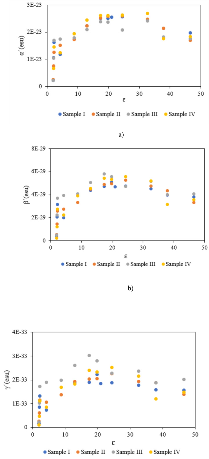
The changes of (a) α’, (b) β’, and (c) γ’ of used samples based on of dielectric constant of selected solvents.

Biomolecules’ hyperpolarizability (β’) in the first order

Oudar’s famous equation is a simple way to measure the nonlinearity of sample solutions. The Two-level model explains the relationship between the molecular hyperpolarizability parameter and changes in dipole moments (Δµ), and dipole transition (µ_e.g.) as follows^39–41:

5

In above equation, υ_L is the reference incident beam’s frequency. In this research, Δµ was calculated using Lippert Mataga’s model (Table 5, and Table 6). µ_e.g. is also obtained from the oscillator strength data of samples in different environments. Sample III with high differences between dipole moments tend to show high first-order hyperpolarizability. Under this condition, the molecular nonlinear responses are modified by variations in the molecular environment features. As shown in Fig. 9(b), molecular first-order hyperpolarizability is decreased in high-polar solvents such as DMSO.

Biomolecules’ hyperpolarizability (γ’) in the second order

Compared to first-order calculations, the three-level model is usually used for calculating nonlinear optical hyperpolarizability in the second order. In this case, three different terms are appeared in Eq. 6 for calculating molecular third-order nonlinear hyperpolarizability^42,43.

6

A comparison between Eq. 6 and Eqs. 3, 5 indicates that the second term depends on the dipole transition (µ_e.g.) and transition energy (E_e.g.) similar to Eq. 3, and the first term depends on the dipole transition (µ_e.g.), transition energy (E_e.g.) and changes in dipole moments (Δµ) similar behavior to Eq. 5. In contrast to first and second terms, dipole transition () and energy transition from ground to the second excited state () have the contribution in the molecular higher-order nonlinearity. Hence, by neglecting the third term, the above expression can be rewritten according to Eq. 5 (a quasi-two-level model).

5

As summarized in Table 5, and Table 6, sample III with high Δµ indicates high second-order hyperpolarizability compared to other samples. In general, charge distribution and molecular electronic structure are modified differently in environments with different polarity features. As shown in Fig. 9 (c), different nonlinear behaviors occur in low and high-polar solvent environments. For environments with ɛ < 21, by increment dielectric factor of solvents, molecular hyperpolarizability in the second order is enhanced. In opposite behaviors, the molecular nonlinear responses are decreased in environments with ɛ ˃ 21. In this case, in competition between various solute-solvent interactions, sample III with the methoxy group indicates high nonlinearity. The results display the same effects of solvents on the biomolecules’ linear polarizability, and their hyperpolarizability in the first and second order. Although, this qualitative study gives main data about environment polarity effects on the biomolecules’ nonlinear features, the studies on the contribution of each environment polarity effect will be helpful. In this case, multi-linear analysis is used similarly to Sect. 3.2. According to Data in Tables 9 and 10, specific solute-solvent interactions have an important effect on the molecular hyperpolarizability. Although environments with strong hydrogen bond acceptor features are increased the nonlinear optical behaviors of sample I, nonlinearity of other samples is enhanced in environments with high hydrogen bond donor abilities. So, a correct selection of polarity features of environments surrounding understudy molecules can enhance their nonlinear optical responses.

Table 9.

Regression fit to Kamlet-Abboud-Taft polarity scales for hyperpolarizability of used samples in first order with percentage contribution of various solvent interactions.

Multi-parameter scale	ν0 (cm− 1) x 10− 29	a (cm− 1) x 10− 29	b (cm− 1) x 10− 29	c (cm− 1) x 10− 29	R 2
Sample I
β’	0.661 ± 0.693	1.069 ± 0.908	3.047 ± 1.231	1.341 ± 1.165	0.75
Sample II
β’	0.742 ± 0.774	2.611 ± 1.014	1.172 ± 1.375	1.943 ± 1.301	0.72
Sample III
β’	1.579 ± 0.644	1.913 ± 0.852	1.370 ± 1.141	1.962 ± 1.079	0.75
Sample IV
β’	0.948 ± 1.214	3.816 ± 1.053	-0.044 ± 1.473	2.182 ± 1.666	0.73
	Multi-parameter scale	Pα(%)	Pβ(%)	Pπ*(%)
	Sample I
	β’	20	56	24
	Sample II
	β’	46	20	34
	Sample III
	β’	37	26	37
	Sample IV
	β’	63	1	36

Table 10.

Regression fit to Kamlet-Abboud-Taft polarity scales for hyperpolarizability of used samples in second order with percentage contribution of various interactions.

Multi-parameter scale	ν0 (cm− 1) x 10− 34	a (cm− 1) x 10− 34	b (cm− 1) x 10− 34	c (cm− 1) x 10− 34	R 2
Sample I
γ’	0.255 ± 0.287	0.446 ± 0.375	1.272 ± 0.509	0.525 ± 0.482	0.75
Sample II
γ’	0.299 ± 0.328	1.093 ± 0.430	0.483 ± 0.584	0.849 ± 0.552	0.71
Sample III
γ’	0.749 ± 0342	0.900 ± 0.452	0.873 ± 0.605	0.817 ± 0.572	0.74
Sample IV
γ’	0.363 ± 0.524	1.778 ± 0.455	-0.125 ± 0.636	0.978 ± 0.720	0.75
	Multi-parameter scale	Pα(%)	Pβ(%)	Pπ*(%)
	Sample I
	γ’	20	57	23
	Sample II
	γ’	45	20	35
	Sample III
	γ’	35	34	31
	Sample IV
	γ’	62	4	34

Moreover, a comparison between the nonlinear optical properties of 1-Indanone compounds with other organic compounds indicates that indanone derivatives tend to indicate high second-order nonlinear responses in comparison to other molecules such as coumarins, azo compounds, carbazole-based compounds, and pyrazole^44–49. Therefore, 1-Indanone compounds can be considerd as an excellent material for designing nonlinear optical devices.

Conclusions

In this experimental research, the polarity effects on the optical characteristics of 1-Indanone compounds were studied in linear and nonlinear domains. According to the results, the features of the environment surrounding biomolecules have vital roles in their optically important properties. In addition to a qualitative study, the polarity-based models were used to find dominant environment polarity effects. Despite the significant contribution of general interactions on the biomolecules’ ground state, there is considerable competition between general and specific environment-induced effects on their excited state. In contrast to samples II and IV, specific molecular interactions show a dominant effect in the excited state of sample I, and sample III. In real, these differently appeared behaviors are due to various activities of substituents in biomolecular structure.

Moreover, polarity-based models provide a simple way for estimating different environmental effects on biomolecules’ optical nonlinearity. Based on the results, environment polarity has the same effect on molecular hyperpolarizability in the first and second order. Therefore, the primary studies on the environmental effects on the first-order nonlinearity of biomolecules can give helpful information about their higher-order nonlinearity.

Electronic supplementary material

Below is the link to the electronic supplementary material.

Author contributions

All authors contributed to the study conception and design. Sample preparation was performed by Z. Sayyar, R. Teimuri-Mofrad, and K. Rahimpour. Experimental analysis was performed by M. Khadem Sadigh. Theoretical analysis was performed by A. N. Shamkhali. The first draft of the manuscript was written by M. Khadem Sadigh. All authors read and approved the final manuscript.

Funding

No funding sources.

Data availability

All data generated or analyzed during this study are included in this published article.

Declarations

Competing interests

The authors declare no competing interests.

Ethics approval and consent to participate

Not applicable.

Consent for publication

Not applicable.

References

- 1.Tang, M. L., Zhong, C., Liu, Z. Y., Peng, P. & Sun, X. Discovery of novel sesquistilbene indanone analogues as potent anti-inflammatory agents. Eur. J. Med. Chem.113, 63–74 (2016). [DOI] [PubMed] [Google Scholar]
- 2.Sheng, R. et al. Design, synthesis and AChE inhibitory activity of indanone and aurone derivatives. Eur. J. Med. Chem.44, 7–17 (2009). [DOI] [PubMed] [Google Scholar]
- 3.Charris, J. E. et al. Synthesis and antimalarial activity of (E)2-(2ˊ-chloro-3ˊ-quinolinylmethylidene)-5, 7-dimethoxyindanones, Lett. Drug Des. Discov. 4, 49–54 (2007). [Google Scholar]
- 4.Finkieisztein, L. M. et al. New 1-indanone thiosemicarbazone derivatives active against BVDV. Eur. J. Chem.43, 1767–1773 (2008). [DOI] [PubMed] [Google Scholar]
- 5.Gomez, N. et al. Synthesis, structural characterization, and pro-apoptotic activity of 1-Indanone thiosemicarbanzone platinum (II) and palladium (II) complexes: Potential as antileukemic agents. Chem. Med. Chem.6, 1485–1494 (2011). [DOI] [PubMed] [Google Scholar]
- 6.Hammen, P. D. & Miline, G. M. US Patent4164514 (1979).
- 7.Sindelar, R. D. et al. 2-Amino-4, 7-dimethoxyindan derivatives: Synthesis and assessment of dopaminergic and cardiovascular actions. J. Med. Chem.25, 858–864 (1982). [DOI] [PubMed] [Google Scholar]
- 8.Saxena, H. O. et al. Gallic acid-based indanone derivatives as anticancer agents. Bioorg. Med. Chem. Lett.18, 3914–3918 (2008). [DOI] [PubMed] [Google Scholar]
- 9.Ahmed, N. Synthetic advances in the indane natural product scaffolds as drug candidates: A review. Elsiver. 51, 383–434 (2016). Studies in natural products chemistry. [Google Scholar]
- 10.Patil, S. A., Patil, R. & Patil, S. A. Recent developments in biological activities of indanones. Eur. J. Med. Chem.138, 182–198 (2017). [DOI] [PubMed] [Google Scholar]
- 11.Reichardet, C. Solvents and Solvent Effects in Organic Chemistry, 3rd ed (Wiley-VCH Verlag GmbH & Co. KGaA, 2003).
- 12.Solomonov, B. N., Varfolomeev, M. A. & Abaidullina, D. I. Solvent effect on H-bond cooperativity factors in ternary complexes of methanol, octan-1-ol, 2,2,2-trifluoroethanol with some bases. J. Spectrochim Acta Mol. Biomol. Spectrosc., 985–990 (2008). [DOI] [PubMed]
- 13.Yao, E. & Acree, W. E. Jr Abraham model solute descriptors for favipiravir: Case of tautomeric equilibrium and intermolecular hydrogen-bond formation. Thermo. 3, 443–451 (2023). [Google Scholar]
- 14.Khadem Sadigh, M., Zakerhamidi, M. S., Shamkhali, A. N., Shabani, B. & Rad-Yousefinia, N. Investigation on environmental sensitivity characteristics of pyridine compounds with different position of N-atoms and various active functional groups. J. Mol. Liq.275, 926–940 (2018). [Google Scholar]
- 15.Khadem Sadigh, M. & Zakerhamidi, M. S. Solvent polarity sensitive characteristics of various tautomers of azo compounds: Linear and nonlinear optical properties. Spectrochemica Acta Part. A: Mol. Biomol. Spectrosc.239, 118445 (2020). [DOI] [PubMed] [Google Scholar]
- 16.Khadem Sadigh, M., Hasani, H. & Rahimpour, J. Media polarity and substituent effects on the photo-physical properties of some nickel complexes with azo-azomethine. J. Mol. Struct.1212, 128122 (2020). [Google Scholar]
- 17.Kamlet, M. J. & Taft, R. W. Linear solvation energy relationships, part 3, some reinterpretations of solvent effects based on correlations with solvent effects based on correlations with π* and α values. J. Chem. Soc. Perkin Trans.2, 349–356 (1979). [Google Scholar]
- 18.Kamlet, M. J. & Taft, R. W. The solvatochromism comparison method. I. the beta-scale of solvent hydrogen-bond acceptor (HBA) basicities. J. Am. Chem. Soc.98, 377–383 (1976). [Google Scholar]
- 19.Abboud, J. L., Kamlet, M. J. & Taft, R. W. Regarding a generalized scale of solvent polarities. J. Am. Chem. Soc.99, 8325–8327 (1977). [Google Scholar]
- 20.Catalan, J. Toward a generalized treatment of the solvent effect based on four empirical scales: Dipolarity (SdP, a new scale), polarizability (SP), acidity (SA), and basicity (SB) of medium. J. Phys. Chem. B. 113, 5951–5960 (2009). [DOI] [PubMed] [Google Scholar]
- 21.Wypych, G. Handbook of Solvents, 2nd edn (Chem Tec., Torento, 2014).
- 22.Mozaffarinia, S., Teimuri-Mofrad, R. & Rasidi, M. R. Design, synthesis and biological evaluation of 2,3-dihydro-5,6-dimethoxy-1H-inden-1-one and piperazinium salt hybrid derivatives as hAChE and hBuChE enzyme inhibitors. Eur. J. Med. Chem.191, 112140 (2020). [DOI] [PubMed] [Google Scholar]
- 23.Rahimpour, K., Nikbakht, R., Aghaiepour, A. & Teimmuri-Mofrad, R. Synthesis of 2-(4-amino substituted benzylidene indanone analogues from aromatic nucleophilic substitution (SNAr) reaction. Synth. Commun.48, 2253–2259 (2018). [Google Scholar]
- 24.Yanai, T., Tew, D. & Handy, N. A new hybrid exchange-correlation functional using the Coulomb-attenuating method (CAM-B3LYP). Chem. Phys. Lett.393, 51–57 (2004). [Google Scholar]
- 25.McLean, A. D. & Chandler, G. S. Contracted gaussian-basis sets for molecular calculations. 1. 2nd row atoms, Z = 11–18. J. Chem. Phys.72, 5639–5648 (1980). [Google Scholar]
- 26.Sosa, C. et al. A local density functional study of the structure and vibrational frequencies of Molecular Transition-Metal compounds. J. Phys. Chem.96, 6630–6636 (1992). [Google Scholar]
- 27.Simon, S., Duran, M. & Dannenberg, J. J. How does basis set superposition error change the potential surfaces for hydrogen bonded dimers? J. Chem. Phys.105, 11024–11031 (1996). [Google Scholar]
- 28.Marenich, A. V., Cramer, C. J. & Truhlar, D. G. Universal solvation model based on solute electron density and a continuum model of the solvent defined by the bulk dielectric constant and atomic surface tensions. J. Phys. Chem. B. 009, 113, 6378–6396 (2009). [DOI] [PubMed] [Google Scholar]
- 29.https://comp.chem.umn.edu/solvation/mnsddb.pdf
- 30.Furche, F. & Ahlrichs, R. Adiabatic time-dependent density functional methods for excited state properties. J. Chem. Phys.117, 7433–7447 (2002). [Google Scholar]
- 31.Onsager, L. Electric moments of molecules in liquids. J. Am. Chem. Soc.58, 1486–1493 (1936). [Google Scholar]
- 32.Valiev, M. et al. NWChem: A comprehensive and scalable open-source solution for large scale molecular simulations. Comput. Phys. Commun.181, 1477 (2010). [Google Scholar]
- 33.Ghanadzadeh Gilani, A., Moghadam, M., Hosseini, S. E. & Zakerhamidi, M. S. A comparative study on the aggregate formation of two oxazine dyes in aqueous and aqueous urea solutions. Spectrochim Acta Mol. Biomol. Spectrosc.83, 100–105 (2011). [DOI] [PubMed] [Google Scholar]
- 34.Khadem Sadigh, M. & Zakerhamidi, M. S. The roles of solute-solute and solute-solvent interactions on the nonlinearity of aqueous solutions of ionic dyes. Z. fur Naturforschung A. 73, 785–794 (2018). [Google Scholar]
- 35.Tajalli, H., Ghanbarzadeh Gilani, A., Zakerhamidi, M. S. & Moghadam, M. Effects of surfactants on the molecular aggregation of rhodamine dyes in aqueous solutions, 72 697–702. (2009). [DOI] [PubMed]
- 36.Prlj, A., Curchod, B. F. E., Fabrizio, A., Floryan, L. & Corminboeuf, C. Qualitatively incorrect features in the TDDFT spectrum of thiophene-based compounds. J. Phys. Chem. Lett.6, 13–21 (2015). [DOI] [PMC free article] [PubMed] [Google Scholar]
- 37.Lippert, E. Spektroskoische Bestimmung Des Dipolmmoments aromatischer Verbindungen Im Ersten Angeregten Singulettzustand. Z. Fur Elektrochemie Berichte Der Bunsengesellschaft Fur Phys. Chem.61, 962–975 (1957). [Google Scholar]
- 38.Cbeng, L., Tam, W., Sevenson, S. H., Meredith, G. R. & Marder, S. R. Experimental investigation of organic molecular nonlinear optical polarizabilities.1. Methods and results on benzene and stilbene derivatives. J. Phys. Chem.95, 10631–10643 (1991). [Google Scholar]
- 39.Zakerhamidi, M. S., Moghadam, M. & Karimi, A. Aggregative properties of Phodamine dyes in polyacrylamide hydrophilic gel media. J. Mol. Struct.1033, 289–297 (2013). [Google Scholar]
- 40.Oudar, J. L. & Chmla, D. S. Hyperpolarizabilities of the nitroanilines and their relations to the excited state dipole moment. J. Chem. Phys.66, 2664 (1977). [Google Scholar]
- 41.Momicchioli, F., Ponterini, G. & Vanossi, D. First- and second order polarizabilities of simple mercocyanines, an experimental and theoretical reassessment of the two-level model. J. Phys. Chem. A. 112, 11861–11872 (2008). [DOI] [PubMed] [Google Scholar]
- 42.Carlotti, B., Flamini, R., Kikas, I., Mazzucato, U. & Spalletti, A. Intramolecular charge transfer, solvatochromism and hyperpolarizability of compounds bearing ethynylene or ethylene bridges. Chem. Phys.407, 9–19 (2012). [Google Scholar]
- 43.Paley, M. S. et al. A solvatochromic method for determining second order polarizabilities of organic molecules. J. Org. Chem.54, 3774–3778 (1989). [Google Scholar]
- 44.Dirk, C. W., Cheng, L. T. & Kuzyk, M. G. A simplified three-level model describing the molecular third order optical susceptibility. Int. J. Quantum Chem.43, 27–36 (1992). [Google Scholar]
- 43.Warde, U. & Sekar, N. Solvatochromic benzo [h] coumarins: Synthesis, solvatochromism, NLO and DFT study. J. Opt. Mater.72, 346–358 (2017). [Google Scholar]
- 45.Warde, U. & Sekar, N. NLOphoric mono-azo dyes with negative solvatochromism and in-built ESIPT unit from ethyl 1,3-dihydroxy-2-naphthoate: Estimation of excited state dipole moment and pH study. Dyes Pigm.137, 384–394 (2017). [Google Scholar]
- 46.Kadam, M. L., Patil, D. & Sekar, N. Fluorescent carbazole based pyridine dyes synthesis, solvatochromism, linear and nonlinear optical properties. J. Opt. Mater.85, 308–318 (2018). [Google Scholar]
- 47.Thorat, K. G., Ray, A. K. & Sekar, N. Modulating TICT to ICT characteristics of acid switchable red emitting boradizaindacene chromophores: Perspectives from synthesis, photophysical, hyperpolarizability and TD-DFT studies. Dyes Pigm.136, 321–334 (2017). [Google Scholar]
- 48.Lanke, S. K. & Sekar, N. Pyrazole based NLOphores: Synthesis, photophysical, DFT, TDDFT studies. Dyes Pigm.127, 116–127 (2016). [Google Scholar]
- 49.Lanke, S. K. & Sekar, N. Aggregation induced emissive carbazole-based push pull NLOphores: Synthesis, photophysical properties and DFT studies. Dyes Pigm.124, 82–92 (2016). [Google Scholar]
Associated Data
This section collects any data citations, data availability statements, or supplementary materials included in this article.
Supplementary Materials
Data Availability Statement