A dynamic receptive field and improved feature fusion approach for federated learning in financial credit risk assessment

Abstract

Federated Learning (FL) uses local data to perform distributed training on clients and combines resulting models on a public server to mitigate privacy exposure by avoiding data sharing. However, further research indicates that communication overheads continue to be the primary limitation for FL relative to alternative considerations. This is especially true when training models on non-independent and identically distributed data, such as financial default risk data, where FL’s computational costs increase significantly. This study aims to address financial credit risk data by establishing a dynamic receptive field adjustment mechanism for feature extraction, efficiently extracting default features with varying distributions and attributes. Additionally, by constructing a distributed feature fusion architecture, characteristics from both local and overarching models are aggregated to attain higher accuracy with lower transmission costs. Experimental results demonstrate that the proposed FL framework can utilize dynamic receptive fields to allocate convolutional kernel weights, thereby improving feature extraction. In the feature fusion stage, the proposed Multi-Fusion strategy efficiently customizes the aggregation of features from local and global models. The final solution reduces the communication rounds in federated learning by approximately 80%.

Introduction

In situations where data is dispersed among multiple clients, each processing its own local private data, traditional centralized machine learning methods typically necessitate all data onto a single server for training^1,2. This approach poses privacy and data transmission risks. Federated learning addresses data privacy issues by training models across a distributed network of numerous client devices and sharing distributed model parameters instead of raw data^3–5. By performing local training using client data and subsequently aggregating the trained models on a central server, federated learning mitigates privacy exposure. federated learning has found extensive applications in fields such as financial services^6,7, healthcare⁸, the Internet of things^9,10, and recommendation systems¹¹.

One notable application in the financial services sector is the assessment of credit card fraud, where machine learning models are employed to detect fraudulent transactions. Credit card fraud occurs when an unauthorized party uses someone’s credit card information to make purchases or access funds. This activity presents severe financial risks for both individuals and institutions. However, the imbalanced nature of fraud detection datasets—where fraudulent cases are significantly fewer than legitimate transactions—can reduce the effectiveness of traditional machine learning models^12–14. Moreover, the diversity in feature types and the existence of non-independent and identically distributed (non-IID) data in credit datasets present significant challenges to federated learning algorithms’ accuracy^15,16.

The increasing complexity and volume of credit transactions, combined with evolving fraud tactics, have made it imperative for financial institutions to improve the accuracy of fraud detection models. Traditional centralized approaches often fail to scale effectively while maintaining data privacy, creating a critical need for advanced decentralized methods like federated learning that can operate under privacy constraints without compromising model performance. Addressing the challenge of imbalanced and non-IID data is crucial, as ineffective detection could lead to substantial financial losses and erode customer trust.

The heterogeneity of non-IID data manifests through differences in feature distributions across devices or nodes, as well as uneven label distribution, where some devices may only contain a subset of the overall categories. Such inconsistencies in local model updates can lead to conflicting parameter updates, hindering the convergence of the global model. Addressing non-IID data requires more complex policy designs or multiple communications between clients and the central server to ensure effective training. This increased computational complexity adds further challenges to federated learning implementations ^17–20.

In addition to the challenges of data heterogeneity, the computational and communication burdens associated with federated learning must be addressed to make it a practical solution in real-world financial environments. The frequent transmission of model parameters and feature information between clients and the central server can result in significant communication costs, further highlighting the need for optimization in the feature extraction and fusion processes.

In federated learning, the computational burden largely arises from the frequent transmission of model parameters or feature information between clients and the serve^21,22. The core principle of federated learning is to keep data on local devices, allowing each device to train a model independently and only send model parameters, such as weights and gradients, to the server for aggregation. Enhancing the efficiency of feature extraction is crucial as it allows devices to extract useful information more effectively, resulting in more compact and representative features. This efficiency reduces the dimensionality of the features, thereby decreasing the amount of data that needs to be transmitted, which lowers communication costs and bandwidth consumption^23–25.

Efficient feature extraction also accelerates the federated learning process by allowing clients to quickly identify and use important features locally, minimizing the transmission of unnecessary data^26–28. Moreover, by reducing noise and redundant information, efficient feature extraction improves model accuracy and performance, particularly in handling complex tasks^28,29. Overall, optimizing the feature extraction process enhances the performance and scalability of federated learning systems, making them more suitable for managing large-scale, heterogeneous data environments.

Given the financial sector’s sensitivity to privacy and efficiency, there is a pressing need for solutions that can not only improve the accuracy of federated learning models but also reduce the communication overhead associated with distributed training. This study introduces a federated learning architecture that focuses on improving feature extraction and fusion processes to address these critical needs.

Evaluating credit risk features from different financial institutions involves two critical steps: feature extraction and fusion ^30–33. Extracting these multi-source credit risk features requires a dynamically adjustable receptive field to better capture both local and global information within the data^34,35. A small receptive field helps capture local credit detail features, while a large receptive field captures global credit features. By dynamically adjusting the receptive field during training, the model can learn richer and more hierarchical feature representations, enhancing feature extraction effectiveness^36–38.

The heterogeneity of credit risk data, stemming from different regions, scenarios, and financial attributes, necessitates a coordinated feature fusion architecture^39,40. Such an architecture aids the federated learning framework in harmonizing distributed training across clients from different financial institutions⁴¹. Integrating features from these diverse sources enables the model to leverage multi-source credit default data, capturing richer and more comprehensive feature information, resulting in better training outcomes and improved model generalization^39,42.

In summary, this study aims to address the challenges of multi-source heterogeneous financial credit risk assessment data by establishing a federated learning architecture that leverages improved feature fusion techniques. The proposed architecture integrates a dynamic receptive field adjustment mechanism for efficient feature extraction and a sophisticated feature fusion strategy to reduce communication costs, thereby enhancing model performance and scalability in financial applications where data privacy and efficiency are paramount.

Basic principles

Federated learning

In federated learning, multiple entities (clients) work together to address machine learning challenges under the management of a global server. Individual client stores its private data locally without exchanging or transferring it, thereby providing a degree of privacy protection for users. The procedural stages of federated learning are outlined below: (1) The global model is distributed by the central server to each client participating in the training. (2) The clients receive the model, update it based on their local data, and upload the modified model to the central node. (3) The central server combines the received models and updates the consolidated model. The iterative process continues until convergence of the model is achieved (See Fig. 1).

Fig. 1.

Federated learning algorithm framework.

Given N clients, learning aims to optimize by minimizing the training loss function F(W) and find the optimal model W:

$$minf(w)=\frac{1}{N}\sum _{i=1}^N{f}_i(w)$$ 1

In the framework, each bank in the diagram (e.g., Bank A, Bank B, Bank C, etc.) represents a client, each holding its own private data. This data cannot be shared with other banks or the central server. Therefore, each bank performs model training locally. First, the banks initialize their local models using the global model parameters provided by the server. These initial model parameters have either been preprocessed or are the result of previous training rounds.

The banks perform multiple rounds of training on their local data. During the training process, each bank uses its local feature extractor to extract features from its local data. Simultaneously, features extracted by the server’s global feature extractor are also used, allowing the training to combine both local and global information. The banks’ local models compute outputs through classifiers, and these outputs are used to calculate the gradients of the loss function. These gradients are used for backpropagation to update the parameters of the local models.

Once the banks complete local training, they compute updated local model parameters (e.g., Model Update (A) for Bank A, Model Update (B) for Bank B, etc.). These model parameter updates (or gradient information) do not directly contain the original data but only include information on how to adjust the model to improve performance. Therefore, the banks can safely send this gradient information to the central server for further processing.

On the server side, after receiving the local model updates or gradients from different banks, federated aggregation is performed. After federated aggregation is completed, the server generates new global model parameters (Global Model Update). These updated parameters reflect the improvements integrated from multiple banks’ models. The new parameters are sent back to the participating banks to be used as the initial model parameters for the next training round. As multiple rounds of federated learning iterations take place, the model performance gradually improves. Ultimately, the global model is used for credit risk assessment. Since this model has been collaboratively trained on data from multiple banks, it generally possesses better generalization capabilities and improved predictive performance.

Squeeze-excitation of extracting feature

The squeeze-excitation attention mechanism is a type of channel-wise attention mechanism that specifically captures the dependencies among feature channels. In the squeeze-excitation networks, the importance of each feature channel is automatically learned, allowing the networks to amplify valuable features and attenuate less relevant features for the current task. Research has shown that incorporating the squeeze-excitation block into various existing classification networks yields significant improvements.

The squeeze-excitation block (Fig. 2) introduces a novel feature recalibration strategy without adding new spatial dimensions for feature channel fusion. Given an input X with c₁ feature channels, a set of convolutional operations and subsequent processing steps produce a feature map with c₂ channels. Unlike traditional Convolutional neural networks (CNNs), the squeeze-excitation block then applies two critical operations squeeze and excitation—to recalibrate the features obtained earlier.

Fig. 2.

The squeeze-excitation networks Structure Diagram. The key operations, squeeze and excitation, automatically learn the importance of feature maps in each channel. This process assigns different weights to different channels, enhancing the contribution of useful channels.

The main difference between the squeeze-excitation mechanism and traditional CNNs lies in how they handle the relationships between feature channels and the adaptability of weights. Traditional CNNs focus on extracting and combining local spatial features through convolution operations, using multiple filters to capture different spatial patterns. However, these operations do not explicitly model the relationships between different feature channels. In contrast, the squeeze-excitation mechanism explicitly models these inter-channel relationships. It adaptively recalibrates the importance of each feature channel, allowing the network to dynamically enhance or suppress specific features based on their relevance to the task.

Another key difference is the use of dynamic weights. In traditional CNNs, the weights of convolutional filters are static, meaning they remain unchanged after training and apply the same weights to all input images. However, the squeeze-excitation mechanism introduces a dynamic weight adjustment mechanism. For each input image, the squeeze-excitation mechanism generates a set of adaptive feature channel weights based on the global semantic information of the image. This dynamic property allows the model to flexibly respond to changes in input data, enhancing the model’s generalization ability across different tasks and datasets.

The Squeeze operation compresses features across the extent, reducing a high-dimensional representation into a single scalar with an overarching receptive field, which is that the representation is derived from the entire input space, providing a broad overview of the data. The resultant dimension aligns with the initial feature channel count, ensuring that the overall distribution responds to the feature channels, enabling even the layers near the input to have a global receptive feature.

The resultant dimension aligns with the initial feature channel count, ensuring that the overall distribution responds to the feature channels, enabling even the layers near the input to have a global receptive field, allowing the network to access information from the entire input, not just a local region.

The Excitation operator functions similarly to a gating mechanism in recurrent neural networks. It assigns trainable weights w to each feature channel, explicitly modeling the interdependencies between feature channels. The network adjusts these weights based on the loss function, prioritizing greater importance to valuable feature representations and diminishing the importance of less valuable ones, thereby enhancing the model’s performance.

The Excitation operator uses a new neural network (comprising two linear layers) to learn from the channel-wise data (processed independently on each feature channel), which is then multiplied with the original channel data. This operation provides more nonlinear fitting capability, allowing for a better capture of complex inter-channel relationships. The output weights from the Excitation operator represent the significance of individual channel post feature selection. By multiplying these weights with the initial data channel-wise, the initial data is recalibrated along the channel dimension.

Contribution

This study aims to address the challenges associated with multi-source heterogeneous financial credit risk assessment data by establishing a novel federated learning architecture that leverages an improved feature fusion technique. Unlike traditional federated learning approaches that often struggle with data heterogeneity and limited model generalization, our method introduces a dynamic receptive field adjustment mechanism during feature extraction, which allows for more precise and efficient identification of credit default features across diverse data sources. This mechanism adapts to varying data distributions and feature importance, providing a tailored extraction process that enhances model performance on complex, real-world financial datasets.

In addition to the innovative feature extraction process, our study also introduces an advanced feature fusion strategy that aggregates features from both local and global models in a more cohesive manner. This approach not only mitigates the issues of data distribution disparities but also significantly reduces communication costs—a common bottleneck in federated learning. By ensuring that the most relevant and representative features are effectively fused, the proposed architecture enhances the robustness and accuracy of the credit risk assessment models, making it more suitable for financial applications where data privacy and efficiency are critical.

Compared to existing works, which often rely on static and less adaptive methods for feature extraction and fusion, our approach provides a more dynamic and scalable solution (Table 1), a comparison of problems, prior research gaps, and our proposed approach). The integration of the dynamic receptive field adjustment mechanism with an optimized feature fusion process marks a substantial contribution to the field of federated learning, particularly in financial credit risk assessment. The proposed framework not only addresses the challenges of data heterogeneity and communication overhead but also enhances the model’s ability to generalize across different datasets, thereby providing a more reliable and efficient tool for assessing credit risk in a federated learning environment.

Table 1.

Comparison of problems, gaps in prior research, and the proposed federated learning approach.

Problem	Previous research	Proposed approach	Results/Impact
Data heterogeneity	Traditional federated learning methods struggle with non-IID data, leading to reduced model performance due to inconsistent local updates	Dynamic receptive field adjustment mechanism for feature extraction that adapts to varying data distributions and feature importance	Enhances model performance by capturing both local and global credit risk features effectively, overcoming the challenges posed by non-IID data distributions
Limited generalization of models	Models trained in federated learning frameworks often show poor generalization across diverse datasets due to inconsistent data distribution	Aggregates local and global features using a novel feature fusion strategy to ensure cohesive model updates across clients	Improves model generalization across different financial institutions’ datasets, providing more reliable credit risk assessments
Communication overhead	High transmission of model parameters between clients and servers increases communication costs and latency in federated learning frameworks	Efficient feature fusion strategy that reduces the volume of transmitted data by fusing only the most relevant features	Lowers communication costs and reduces bandwidth consumption, making federated learning more scalable and efficient in large financial networks
Static feature extraction and fusion	Prior approaches use static methods for feature extraction and fusion, which are less adaptive to real-world data complexities	Dynamic, adaptive feature extraction and fusion processes that can adjust to the varying nature of financial datasets	Provides a more flexible, scalable, and efficient solution for handling complex, real-world financial data with improved model accuracy and performance
Privacy and security	Centralized approaches increase privacy risks by transferring raw data to a central server	Federated learning architecture keeps data on local devices, sharing only model parameters	Ensures higher data privacy by minimizing data exposure during model training and parameter sharing

Multi-branch attention mechanism

The idea of squeeze-excitation networks is to automatically learn feature weights using a fully connected network based on loss, rather than directly assigning weights based on feature channel values. This approach increases the weights of effective feature channels. However, embedding this module into existing classification networks inevitably adds some parameters and computational overhead. Additionally, capturing dependencies between all channels is inefficient and often unnecessary.

To better adapt federated learning algorithms to individual user distributions, this paper combines feature embedding with personalized user models by introducing a multi-branch attention mechanism into the federated learning framework (Fig. 3). Under this framework, users can select the most appropriate model parameters based on their own data. To ensure training efficiency and accuracy, model parameters can be pre-trained without leaking raw data or compromising privacy. Finally, iterative training is conducted within each participant’s environment.

Fig. 3.

Structure diagram of the selective kernel mechanism. Split: The feature map is divided into multiple branches, each using a different convolutional kernel (resulting in different receptive fields) for extracting feature. Fuse: The features obtained from multiple branches are summed together. Select: Multiple feature vectors, processed by softmax, are multiplied by the feature maps extracted in the first step from the different branches.

The multi-branch attention mechanism enhances the flexibility and representational capacity of the model by introducing multiple parallel attention branches to model and optimize different types of features. This design enables the model to learn the relationships between features in a more fine-grained manner, improving its ability to handle complex data.

In terms of implementation, the multi-branch attention mechanism starts by setting up the branches. This mechanism divides the attention computation into multiple independent branches, each calculating a set of feature weights. These branches can have different parameter settings or network structures to capture various types of features in the input feature map. Each branch applies a different operation to the input feature map, generating a set of weights used to reweight the channels of the input feature map. Then, in the branch output merging stage, the attention weights from different branches are combined using operations like weighted averaging, summation, or concatenation. This step produces the final channel weights, which are used to adjust the channel responses of the input feature map. Finally, in the weight application stage, the fused weights are used to reweight each channel of the original input feature map, to fine-tuning the importance of each channel, allowing the network to better process different features in the input data.

The core principle of the multi-branch attention mechanism lies in capturing different feature patterns. By utilizing multiple parallel attention branches, the model can specialize in processing features across different dimensions. Each branch can be responsible for capturing different types of features, such as edges, textures, or colors, which may be more relevant to specific tasks or datasets. Additionally, the multi-branch mechanism enhances the model’s representational capacity and flexibility, enabling more fine-grained optimization in the feature space. Each branch provides a unique perspective on understanding the input data, allowing the model to perform better on more complex and diverse datasets, thereby improving its generalization ability. Although introducing multiple attention branches increases computational complexity, each branch focuses on different feature types, making the model more efficient in learning and utilizing features overall. This selective learning approach ensures more efficient resource utilization while reducing unnecessary computations.

Dynamic receptive fields

Dynamic receptive field refers to the model adaptively adjusting the size or weight distribution of its receptive field based on different input features during operation. Compared to static receptive fields (i.e. fixed size and weight receptive fields), dynamic receptive fields can more flexibly capture the diversity of input data and enhance the performance of the model.

To improve the efficiency of channel feature capture in squeeze-excitation networks, the module can be extended with multiple branches, each having a different receptive field. This module learns feature embedding functions in the distributed representation space based on personalized user characteristics. The selective kernel mechanism guides the module in determining which user datasets should be used for training model parameters. Additionally, the proposed module embeds personalized user features into the distributed representation space, (c, h, w) → (n, c, h, w), guiding the model to learn more efficient distributed parameter estimators to enhance the effectiveness of the entire federated learning networks.

Each feature map {U_i, i = 1,2,…,N_u} can be embedded into the global feature map S through global average pooling (GAP). The embedding process can be represented as: (n, c, h, w) → (c, h, w) → (c, 1, 1).

$$S_c=F_{\mathit{gap}}\left(U_c\right)=\frac{1}{H·W}\sum _{i=1}^H\sum _{j=1}^W{U}_c(i,j)$$ 2

where, the global feature map S has a shape of 1 × 1 × C, F_gap denotes the global average pooling fusion operator. H and W denote the height and width of the feature map.

The obtained global feature S is passed through a fully connected layer (FC) to reduce its dimensionality, producing a d × 1 (denoted as Z in the figure). This process is represented as:

$$Z=F_{\mathit{fc}}(s)=\delta (F_{\mathit{bn}}(W_s))$$ 3

where, F_fc denotes the fully connected layer function, δ is the ReLU activation function, F_bn is the batch normalization function, and W represents the weight matrix of size d × c:

$$d=\text{max}\left(c/r,L\right)$$ 4

where r is the scaling ratio and L is the minimum value of d.

Next, N_u fully connected layers are used for dimensionality expansion, resulting in N_u feature maps with the same dimensions as before the reduction. The N_u feature vectors undergo softmax processing, yielding N_u feature maps of dimensions (c, 1, 1). When N_u = 2, softmax processing yields a and b as follows:

$$e_i=e^{E_c^{i}Z}\left./\phantom{e^{E_c^{i}Z}\sum _i^{N_u}{e}^{E_c^{i}Z}}\right)\sum _i^{N_u}{e}^{E_c^{i}Z}$$ 5

where, e_i has dimensions (c, 1, 1). E ∈ R^d×c; E_c ∈ R^1×d represents the c-th row of E.

After applying softmax to multiple feature vectors, each vector is multiplied by the feature maps U_i extracted from multiple branches in feature separation. The feature dimensions change to N_u (c,1,1) * N_u (c, h, w) = (N_u, c, h, w). Finally, the n feature maps are summed up, represented as:

$$V_c=\sum _{i=1}^{N_u}{e}_c^i·U_c^i$$ 6

After the central global node transmits the model weights w^t_g to the k-th (k = 1,2,..,N_k) client, the client batch training can be represented as:

$$w_{k,b+1}^t=w_{k,b}^t-\eta \lambda \left(w_{k,b}^t-{\theta }_k(w_{k,b}^t)\right)$$ 7

where b denotes the client’s training round, N_b is the total count of training iterations, η controls the learning rate, and λ is a hyperparameter to be trained.

In machine learning, the learning rate (η) and hyperparameter (λ) are key factors that influence the effectiveness of model training. The learning rate determines the size of the step by which the model adjusts its weights in each iteration: a higher learning rate speeds up training but may lead to instability, while a lower learning rate makes training more stable but potentially too slow. The hyperparameter (λ) is often used for regularization, by adding a penalty term to the loss function to prevent overfitting. A larger λ value simplifies the model and reduces the risk of overfitting, but may cause underfitting, whereas a smaller λ value makes the model more complex and increases the risk of overfitting. In federated learning, the settings of η and λ not only affect the training on individual clients but also the global model. Therefore, they need to be dynamically adjusted based on the training conditions to achieve optimal results.

Deformable convolution

Deformable convolution (DeConv) is a specialized convolution operation that allows the convolution kernel (ConvK) to dynamically deform on the input feature map to adapt to irregular receptive fields. Traditional convolution operations use fixed kernel shapes (typically rectangles), whereas DeConv dynamically modifies the size and location of the convolution kernel based on the content of the input tensor, thereby effectively representing complex image features.

Compared to traditional convolutions, which extract features within a fixed rectangular window, DeConv can capture more complex spatial relationships within the receptive field. DeConv extends beyond image data and is applicable to diverse forms of unstructured data, particularly suitable for applications such as financial risk assessment to enhance the flexibility and efficiency of feature extraction.

The structure of traditional convolution is characterized by:

$$y(p_0)=\sum _{p_n\in R}\left(w(p_n)·x(p_0+p_n)\right)$$ 8

here p₀ denotes each location in the feature outputting map aligned with the central position of the Conv K, p_n is the offset of p₀ across the Conv K size, R denotes the index of each block, w(p_n) are the weights, and x(p₀ + p_n) denotes the original sample.

DeConv introduces an offset Δp_n for each sub-region point to achieve deformation based on Eq. (8). Δp_n is iteratively improved through end-to-end learning, starting from random initialization and updated after each iteration. The DeConv can be represents as:

$$y(p_0)=\sum _{p_n\in R}\left(w(p_n)·x(p_0+p_n)\right)$$ 9

Since the coordinates after adding offsets are usually not integers corresponding to actual feature points on the feature map, interpolation methods are needed to obtain the feature values after offsetting. A commonly used interpolation method is bilinear interpolation, which linearly interpolates data features in different directions to calculate the actual sampled values.

Global–local fusion (GLF)

During the t-th round of training, clients retain the global feature extractor E_g sent by the server. When iterating updates in the local classifier, they consider fusing E_g with E_l. During local training, the model’s features are not merely local; they integrate features extracted by the overarching model’s feature extractor in the prior iteration with local features before training. After fusion, training proceeds. Upon completion, the latest local model weights are sent to the server, at which these parameters undergo exponential moving average aggregation to form updated global parameters.

Throughout training, E_g remains static and a supplementary feature fusion module (Fig. 4) is attached. After training on the client side, the local networks, along with the feature fusion module, is transmitted to the global node for networks combination. Exponential moving average strategy is employed here for smoothing updates.

Fig. 4.

The fusion framework of global and local features in federated learning.

Three types of feature extractors—Single, Multi, and Conv (Fig. 5)—are used to evaluate the effectiveness of feature fusion. Each input data x is processed separately by the individual feature handler E_l and the overarching feature handler E_g. The feature fusion operator F combines the features extracted by both extractors: F(E_l (x), E_g (x)). The fused features are then mapped to R^C×H×W.

Fig. 5.

Different types of feature extractors. The blue parts represent 2-channel features derived from the local module, while the gray parts represent 2-channel features derived from the global module.

Single Operator employs a scalar λ to weight and sum the local and global features. Additionally, the Multi Operator employs a weight matrix λ to weight and sum the local and global features. To perform element-wise multiplication with feature maps, the shape of the λ weight matrix needs adjustment to match the shape of the feature maps.

$$F_{\mathit{single}}\left(E_l\left(x\right),E_g\left(x\right)\right)=\lambda E_g\left(x\right)+(1-\lambda )E_l\left(x\right)$$ 10

$$F_{\mathit{multi}}\left(E_l\left(x\right),E_g\left(x\right)\right)=\mathbf{\lambda }{E}_g\left(x\right)+(1-\mathbf{\lambda })E_l\left(x\right)$$ 11

where, λ is a weighting coefficient used to balance the global feature E_g(x) and the local feature E_l(x) in the fused feature F(E_g(x), E_l(x)). Its value ranges between [0, 1]: when λ = 1, the fusion result completely depends on the global feature; when λ = 0, it completely depends on the local feature; when 0 < λ < 1, it is a weighted average of the two. By adjusting λ, the model can find an optimal balance between global and local features, thus enhancing the flexibility of feature fusion and the model’s expressive capability. In practical applications, λ can be fixed or treated as a learnable parameter, allowing the model to adaptively adjust the feature fusion ratio to optimize performance. Therefore, the selection of λ is crucial for achieving effective feature fusion and improving the overall performance of the model.

After convolution and pooling operations, the feature information obtained by the CNN operator can be expressed as:

$$F_{\mathit{conv}}\left(E_l\left(x\right),E_g\left(x\right)\right)=W_{\mathit{conv}}\left(E_g\left(x\right)||E_l\left(x\right)\right)$$ 12

where, W_conv represents a trainable weight matrix of shape 2C × C. The operation involves concatenating (||) the global features E_g and local features E_l before applying convolution.

Following these operations, the features extracted by the global feature extractor E_g and the local feature extractor E_l are fused into a new feature representation with a shape of R × C × H × W.

Framework

The proposed framework is divided into four parts, with detailed descriptions of each part as follows:

The training framework is structured into two main phases (Table 2): server-side training and client-side training. The server-side processes mainly occur at the beginning and the end of the framework, namely: Server initialization of the model (Step 1) and Server aggregation of model parameters (Step 4).

Table 2.

The proposed federated learning framework process pseudocode.

In Server initialization of the model (Step 1), at the start of training, the server (global model) initializes the model parameters W_0,g and sets the global communication rounds T. In each round of communication, the server randomly selects M clients to participate in that round of training. This random selection helps reduce communication overhead and improve training efficiency. The selected clients will receive the current global model parameters W_t,g, which have been processed with selective kernel enhancement.

In Server aggregation of model parameters (Step 4), after completing all local training rounds, each client calculates and returns the updated local parameter gradients L_t,b+1 to the server. Then, each client sends its updated local model parameters W_t,k back to the server. Upon receiving the local model parameters from all participating clients, the server aggregates these parameters using the EMA method, which computes the new global model parameters W_t+1,g. The EMA method assigns more weight to the model weights from the most recent rounds, better reflecting the latest changes in the model.

In dynamic receptive field fusion (Step 2), during the t-th round update, a random selection of m clients occurs, where each client receives the current global parameters w_g. Clients compute gradients based on these weights and transmit them to the global node. The global node combines these gradients via exponential moving average to update the global parameters to w_g^t+1.

The main tasks for the clients are Client-side feature extraction (Step 2) and Client fusion of local features (Step 3).

In The main tasks for the clients are Client-side feature extraction (Step 2), each selected client performs local training. During local training, each client uses the global model weights W_t,g provided by the server as the initial weights for its local model. The client undergoes multiple rounds of training on its local data N_b. After receiving the global model, each client trains on its local data, using the local feature extractor E_l to extract local features while simultaneously using the global feature extractor E_g to extract global features. For the b-th round of training for the k-th client, the local classifier L is derived from the local feature extractor E_l.

In Client fusion of local features (Step 3), the client calculates local parameters as:

$$L_{t,b}=Cls(F(E_l)),$$ 13

where Cls is the classifier and F is another feature mapping function. During batch training, the client fuses the locally extracted features E_l(x) with the global features E_g(x) provided by the server. This fusion is achieved through different feature fusion operators (refer to Eqs. 10–12). The fused features F(E_l(x), E_g(x)) combine both local and global information. The client then calculates the gradient of the model Co(F(E_l(x), E_g(x))) for each data batch and uses these gradients to perform backpropagation, updating the local model parameters E_l, F, Cls.

In this framework, the dynamic receptive field and deformable convolutions are applied in Step 2 for client-side feature extraction, where local features E_l are extracted. The global–local fusion belongs to the training fusion process, where local fusion is used in Step 3 to merge the client’s local features, while global fusion is applied in Step 4 to aggregate the model parameters on the server side.

This process is repeated until all global communication rounds T are completed or other stopping criteria are met (e.g., model convergence or achieving a predefined training accuracy). After the final round of communication, the global model parameters W_T,g obtained by the server represent the final training result. In this way, federated learning integrates the data from multiple clients for joint model training without directly transmitting raw data, effectively protecting user privacy.

Experiment

Data

We selected 600,000 loan records from a credit platform, comprising 42 variables such as loan amount, loan term, interest rate, installment amount, loan grade, employment title, years employed, homeownership status, annual income, debt-to-income ratio, number of past 2-year credit defaults, number of derogatory public records, and 10 other anonymized variables (See Fig. 6).

Fig. 6.

Partial data distributions in financial credit risk data. (a) Shows the distribution of loan amount. (b) Represents the distribution of loan default status. (c) Depicts the distribution of interest rates. (d) Shows the distribution of installment amount. (e) Illustrates the distribution of variable n2. (f) Displays the distribution of loan grades.

Some of the important fields are as follows: The annualIncome field represents the borrower’s reported annual income, which is used to assess their repayment capacity. applicationType indicates whether the loan application is individual or joint with a co-borrower. dti refers to the debt-to-income ratio, which reflects the proportion of the borrower’s monthly debt payments relative to their monthly income. delinquency_2years records the number of delinquent events (30 days or more past due) in the borrower’s credit history over the past two years. The earliesCreditLine field shows the month when the borrower’s earliest reported credit line was opened. employmentLength indicates the borrower’s employment length, typically measured in years. employmentTitle is the job title provided by the borrower during the loan application. ficoRangeHigh and ficoRangeLow represent the upper and lower limits of the borrower’s FICO score range at the time the loan was issued, with higher scores indicating lower credit risk. grade and subGrade are used to categorize the loan based on the borrower’s credit risk, with subGrade offering further refinement within each grade. homeOwnership reflects the housing status provided by the borrower, such as “Rent” or “Own.” The id field is a unique identifier assigned to each loan record, ensuring that each loan is uniquely identifiable. initialListStatus indicates the initial listing status of the loan. installment refers to the fixed monthly payment amount that the borrower must pay, including both principal and interest. interestRate is the annual interest rate on the loan, indicating the cost of borrowing. issueDate is the month the loan was issued, marking the timeline of the loan’s approval. loanAmnt is the total amount of the loan that the borrower applied for and received. openAcc represents the number of open credit accounts in the borrower’s credit file. pubRec is the number of derogatory public records in the borrower’s credit history, while pubRecBankruptcies reflects the number of public record bankruptcies. purpose describes the loan purpose category selected by the borrower at the time of application, such as “debt consolidation” or “home improvement.” revolBal represents the total revolving credit balance, or the sum of all outstanding balances on revolving credit accounts, while revolUtil indicates the revolving credit utilization rate, which is the amount of credit the borrower has used relative to their total available revolving credit. term is the loan term, typically measured in years, indicating the duration over which the borrower is expected to repay the loan. title is the loan name provided by the borrower, usually a brief description of the loan’s purpose.

The distributions of different credit data vary. For instance, the distribution of anonymized variable n2 primarily concentrates within the range of 0–10, accounting for approximately one-tenth of the overall distribution. The distributions of loan amounts and income follow similar trends, with a predominant presence in the middle-to-low income groups and loan amount bands.

Feature extraction results

To highlight the empirical performance of the proposed feature extraction strategy, selective kernel federated learning (SKF), squeeze-excitation federated learning (SEF), and federated averaging (FedAvg)^43,44 were compared multiple times. Initially, all algorithms were evaluated using the same set of parameters for baseline comparison. Due to varying performances under different hyperparameters, a grid search was conducted to identify the optimal parameter combinations that yielded the highest test accuracy for each algorithm. The accuracy comparison on the financial credit risk dataset is shown in Fig. 7, indicating that SKF’s personalized model outperforms SEF and FedAvg in terms of accuracy.

Fig. 7.

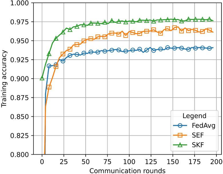
Performance comparison of SKF, SEF, and FedAvg on the financial credit risk dataset.

The training loss convergence curves (Fig. 8a) reveal that SKF starts with the highest initial loss but decreases rapidly, demonstrating the fastest convergence speed and ultimately achieving the lowest training loss, approaching approximately 0.05. This performance indicates excellent training effectiveness with rapid reduction in training loss. SEF starts with a slightly lower initial loss than SKF but exhibits slower descent, converging to a final training loss around 0.1. Overall, SEF shows good training effectiveness but lags behind SKF. FedAvg starts with the lowest initial loss but has the slowest descent rate, resulting in a final training loss of approximately 0.2.

Fig. 8.

The convergence trends of three algorithms on the financial credit risk dataset. (a) Shows the training loss convergence curve. (b) Shows the testing loss convergence curve.

SKF’s faster convergence speed and lower final loss compared to SEF and FedAvg indicate its superior ability to optimize the model during training. SEF demonstrates moderate optimization capability, while FedAvg shows the slowest convergence speed and highest final loss, suggesting poorer training effectiveness and optimization capability.

In testing, SKF initially exhibits the highest test loss but demonstrates the fastest convergence speed (Fig. 8b). After a rapid descent, it achieves the lowest final test loss, approaching around 0.05. This model’s performance on the test set reflects excellent generalization capability. SEF starts with a slightly lower initial test loss compared to SKF but descends slower, converging to a final test loss around 0.1, indicating strong generalization ability. FedAvg, as a reference benchmark, shows the slowest initial test loss descent rate and ends with a final test loss of approximately 0.2, highlighting comparatively weaker generalization among the models.

SKF’s faster convergence speed and lower final test loss compared to SEF and FedAvg demonstrate its superior generalization ability on the test set. SEF follows SKF but with slower convergence speed and slightly higher final test loss. SKF shows rapid descent in both training and test losses, indicating good generalization without overfitting. SEF also exhibits fast descent in both losses but ends with a slightly higher final value than SKF.

In summary, the SKnet algorithm performs the best in federated learning, achieving rapid convergence in both training and testing phases with low losses and strong generalization capability. SEF follows with commendable performance, albeit slightly inferior to SKnet. FedAvg shows comparatively weaker performance and may require model improvements or optimization methods to enhance its performance.

GLF results

To evaluate the effectiveness of the GLF framework in fusing global and local features, we compared the results of GLF_SKF and SKF based on the SKF model (Fig. 9). It is evident that without feature fusion (using the FedAvg method), the model’s performance is the poorest. Among these, the Multi-fusion strategy leads to the highest improvement, followed by the Conv-fusion strategy.

Fig. 9.

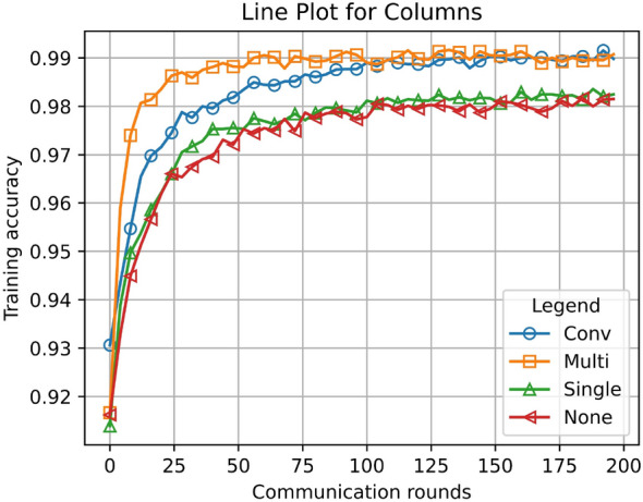
Convergence plots of GLF_SKF and SKF. GLF contains Conv, Multi and Single feature fusion strategy.

To evaluate the performance of three different feature extractors under varying numbers of clients, we applied various test permutations to models with different client counts (Table 3). The table compares the reduction in communication rounds needed to achieve specific accuracies (97% and 98%) relative to the FedAvg method (Table 4). The results show that the SKF + Multi and SKF + Conv strategies significantly reduce the number of communication rounds required.

Table 3.

The convergence precision of SKF across varied configurations.

	Clients number
	5	10	20	50
SKF_None	98.09	94.37	90.29	83.32
SKF + Single	98.26	95.90	91.45	83.85
SKF + Conv	99.04	97.65	95.04	89.21
SKF + Multi	99.19	97.84	95	90.98

Table 4.

Communication iterations to achieve specific precision goals. SKF_None serves as the reference, and decreases in communication iterations are detailed.

	Target acc 98%		Target acc 97%
	Iter	Decrease	Iter	Decrease
SKF_None	101	Ref.	43	Ref.
SKF + Single	93	7.92%	26	39.5%
SKF + Conv	39	61.4%	18	58.1%
SKF + Multi	22	78.2%	8	81.4%

Significant values are in bold.

Regardless of the strategy employed, model performance declines as the number of clients increases. This may be due to increased data diversity and heterogeneity, which poses greater challenges for model training. The SKF_None method performs the worst, indicating that model performance is highly sensitive to the number of clients when no optimization strategy is applied. The SKF + Single strategy shows a slight improvement over SKF_None, indicating some benefit, although the gains are modest. The SKF + Conv strategy demonstrates substantial performance improvements, particularly with fewer clients, highlighting its effectiveness in enhancing model performance. The SKF + Multi strategy consistently delivers the best performance, outperforming other strategies regardless of client count. Its effectiveness is particularly notable with a larger number of clients, demonstrating the Multi strategy’s adaptability and robustness in effectively handling multiple clients.

Overall, incorporating optimization strategies significantly reduces the number of communication rounds required to achieve target accuracy levels. The Multi strategy performs the best, followed by the Conv strategy, and then the Single strategy. SKF_None serves as the baseline method, requiring the most communication rounds. The SKF + Single strategy shows slight improvement, reducing communication rounds by 7.92% and 39.5% to achieve 98% and 97% accuracy, respectively. The SKF + Conv strategy shows significant improvement, reducing communication rounds by 61.4% and 58.1% to achieve 98% and 97% accuracy, respectively. The SKF + Multi strategy performs the best, reducing communication rounds by 78.2% and 81.4% to achieve 98% and 97% accuracy, respectively.

SKF + Multi requires the fewest communication rounds to achieve target accuracy, indicating its highest efficiency. SKF + Conv markedly decreases the needed communication cycles, showing excellent performance. SKF + Single also decreases the needed communication cycles, though not as effectively as Conv and Multi. Compared to SKF_None, all optimization strategies notably reduce the communication cycles needed to attain desired precision, demonstrating their effective enhancement of training efficiency (Table 5).

Table 5.

Comparison of model performance analysis.

Configuration	Precision	Recall	F1 score	AUC-ROC	Convergence speed (Rounds)	Computational overhead (GFLOPs)	Communication overhead (MB)
SKF_None	90.29	88.75	89.51	0.91	150	20.5	15
SKF + Single	91.45	89.65	90.54	0.92	140	22.0	16
SKF + Conv	95.04	94.10	94.57	0.95	130	25.0	18
SKF + Multi	95.00	94.80	94.90	0.96	125	27.5	20

In terms of recall, we observe a similar trend. Recall increases with the upgrade of model configurations, especially in the SKF + Conv and SKF + Multi setups, where these methods perform better at correctly identifying all positive samples. This suggests that the SKF models with convolutional or multi-feature fusion are able to more comprehensively capture the positive sample information in the data, reducing the likelihood of missed detections. The F1 score, which is the harmonic mean of precision and recall, indicates the overall performance of the model in handling imbalanced data. The table shows that both SKF + Conv and SKF + Multi configurations also excel in F1 score, with the SKF + Multi configuration having the highest F1 score, indicating that multi-feature fusion more effectively balances precision and recall. The improvement in AUC-ROC also increases with the enhancement of model configurations, reaching its peak in the SKF + Multi setup. This suggests that more complex feature fusion methods enhance the model’s ability to distinguish between positive and negative samples, providing stronger classification performance.

In terms of convergence speed, more complex model configurations, such as SKF + Multi, show faster convergence, indicating that these methods are able to achieve optimal model performance more quickly. This improvement may be attributed to more efficient feature fusion strategies, enabling the model to learn useful patterns in fewer iterations. However, the computational overhead and communication overhead also significantly increase with the complexity of the model configurations. For example, SKF + Multi has the highest computational and communication overhead. This reflects that although complex feature fusion methods can enhance model performance, they also place higher demands on computational resources and network bandwidth.

Conclusion

This study establishes an improved feature fusion framework within a federated learning architecture. It aims to address financial credit risk data by implementing a dynamic receptive field adjustment mechanism for efficient extraction of default features with diverse distributions and attributes. Moreover, it constructs a distributed feature fusion architecture to aggregate features from local and overarching models, achieving enhance precision with reduced communication costs. Experimental results demonstrate that this method achieves high precision while reducing communication rounds by approximately 80%. Additionally, the feature fusion module provides better initialization for new client data, thereby accelerating the convergence process.

Within the SKF framework, the Selective Kernel strategy effectively captures high-dimensional spatial relationships through adaptive receptive fields, suitable for training unstructured financial credit risk data. In the GLF fusion, the Multi operator provides adaptable selection among local and global feature mappings. The weight vectors consider the proportion of global feature mappings in the respective channels. When there are disparities in client data categories, the Multi operator learns to select the most useful feature mappings.

Author contributions

R.L.: Methodology, Formal analysis, Conceptualization, Writing—original draft, Project administration; Y.C.: Writing—review & editing, Funding acquisition; Y.S.: Writing—review & editing, Investigation; J.G.: Investigation, Supervision, Validation, Writing—original draft, Software; B.S.: Data curation, Software, Visualization, Writing—review & editing; J.Y.: Investigation, Data curation, Validation; Y.D.: Project administration, Resources, Writing—original draft, Validation; Q.Z.: Writing—original draft, Writing—review & editing, Visualization; H.T.: Writing—review & editing, Resources, Investigation.

Funding

The author(s) received no financial support for the research, authorship, and/or publication of this article.

Data availability

The datasets used and/or analyzed during the current study are available from the corresponding author on reasonable request.

Declarations

Competing interests

The author(s) declared no potential conflicts of interest with respect to the research, author-ship, and/or publication of this article.

References

- 1.Guerra, E., Wilhelmi, F., Miozzo, M. & Dini, P. The cost of training machine learning models over distributed data sources. IEEE Open J. Commun. Soc.4, 1111–1126 (2023). [Google Scholar]
- 2.Khan, Q. W. et al. Decentralized machine learning training: A survey on synchronization, consolidation, and topologies. IEEE Access11, 68031–68050 (2023). [Google Scholar]
- 3.Wen, J. et al. A survey on federated learning: Challenges and applications. Int. J. Mach. Learn. Cyber.14, 513–535 (2023). [DOI] [PMC free article] [PubMed] [Google Scholar]
- 4.Jithish, J., Alangot, B., Mahalingam, N. & Yeo, K. S. Distributed anomaly detection in smart grids: A federated learning-based approach. IEEE Access11, 7157–7179 (2023). [Google Scholar]
- 5.Alazab, A., Khraisat, A., Singh, S. & Jan, T. Enhancing privacy-preserving intrusion detection through federated learning. Electronics12, 3382 (2023). [Google Scholar]
- 6.Oualid, A., Maleh, Y. & Moumoun, L. Federated learning techniques applied to credit risk management: A systematic literature review. EDPACS68, 42–56 (2023). [Google Scholar]
- 7.Awosika, T., Shukla, R. M. & Pranggono, B. Transparency and privacy: The role of explainable AI and federated learning in financial fraud detection. IEEE Access12, 64551–64560 (2024). [Google Scholar]
- 8.Coelho, K. K., Nogueira, M., Vieira, A. B., Silva, E. F. & Nacif, J. A. M. A survey on federated learning for security and privacy in healthcare applications. Comput. Commun.207, 113–127 (2023). [Google Scholar]
- 9.Issa, W., Moustafa, N., Turnbull, B., Sohrabi, N. & Tari, Z. Blockchain-based federated learning for securing Internet of Things: A comprehensive survey. ACM Comput. Surv.55, 191:1-191:43 (2023). [Google Scholar]
- 10.Al Asqah, M. & Moulahi, T. Federated learning and blockchain integration for privacy protection in the Internet of Things: Challenges and solutions. Future Internet15, 203 (2023). [Google Scholar]
- 11.Javeed, D. et al. Federated learning-based personalized recommendation systems: An overview on security and privacy challenges. IEEE Trans. Consum. Electron.70, 2618–2627 (2024). [Google Scholar]
- 12.Alonso Robisco, A. & Carbó Martínez, J. M. Measuring the model risk-adjusted performance of machine learning algorithms in credit default prediction. Financ. Innov.8, 70 (2022). [Google Scholar]
- 13.Owusu, E., Quainoo, R., Mensah, S. & Appati, J. K. A deep learning approach for loan default prediction using imbalanced dataset. IJIIT19, 1–16 (2023). [Google Scholar]
- 14.Lagasio, V., Pampurini, F., Pezzola, A. & Quaranta, A. G. Assessing bank default determinants via machine learning. Inf. Sci.618, 87–97 (2022). [Google Scholar]
- 15.Torra, V. A systematic construction of non-i.i.d. Data sets from a single data set: Non-identically distributed data. Knowl. Inf. Syst.65, 991–1003 (2023). [Google Scholar]
- 16.Ma, X., Zhu, J., Lin, Z., Chen, S. & Qin, Y. A state-of-the-art survey on solving non-IID data in federated learning. Future Gener. Comput. Syst.135, 244–258 (2022). [Google Scholar]
- 17.Zhang, H., Zeng, K. & Lin, S. Federated graph neural network for fast anomaly detection in controller area networks. IEEE Trans. Inf. Forensics Secur.18, 1566–1579 (2023). [Google Scholar]
- 18.Paragliola, G. & Coronato, A. Definition of a novel federated learning approach to reduce communication costs. Expert Syst. Appl.189, 116109 (2022). [Google Scholar]
- 19.Kishor, K. Communication-efficient federated learning. In Federated Learning for IoT Applications (eds Yadav, S. P. et al.) 135–156 (Springer International Publishing, 2022). 10.1007/978-3-030-85559-8_9. [Google Scholar]
- 20.Paragliola, G. Evaluation of the trade-off between performance and communication costs in federated learning scenario. Future Gener. Comput. Syst.136, 282–293 (2022). [Google Scholar]
- 21.AbdulRahman, S. et al. Adaptive upgrade of client resources for improving the quality of federated learning model. IEEE Internet Things J.10, 4677–4687 (2023). [Google Scholar]
- 22.Lo, S. K. et al. Architectural patterns for the design of federated learning systems. J. Syst. Softw.191, 111357 (2022). [Google Scholar]
- 23.Mahlool, D. H. & Abed, M. H. A comprehensive survey on federated learning: Concept and applications. In Mobile Computing and Sustainable Informatics (eds Shakya, S. et al.) 539–553 (Springer Nature, 2022). 10.1007/978-981-19-2069-1_37. [Google Scholar]
- 24.Yu, B., Mao, W., Lv, Y., Zhang, C. & Xie, Y. A survey on federated learning in data mining. WIREs Data Min. Knowl. Discov.12, e1443 (2022). [Google Scholar]
- 25.Khan, A., ten Thij, M. & Wilbik, A. Communication-efficient vertical federated learning. Algorithms15, 273 (2022). [Google Scholar]
- 26.Jia, W., Sun, M., Lian, J. & Hou, S. Feature dimensionality reduction: a review. Complex Intell. Syst.8, 2663–2693 (2022). [Google Scholar]
- 27.Maharana, K., Mondal, S. & Nemade, B. A review: Data pre-processing and data augmentation techniques. Glob. Transit. Proc.3, 91–99 (2022). [Google Scholar]
- 28.Zhang, C. et al. Vibration feature extraction using signal processing techniques for structural health monitoring: A review. Mech. Syst. Signal Process.177, 109175 (2022). [Google Scholar]
- 29.Wang, Y., Li, X. & Ruiz, R. Feature selection with maximal relevance and minimal supervised redundancy. IEEE Trans. Cybern.53, 707–717 (2023). [DOI] [PubMed] [Google Scholar]
- 30.Shi, S., Tse, R., Luo, W., D’Addona, S. & Pau, G. Machine learning-driven credit risk: A systemic review. Neural Comput. Appl.34, 14327–14339 (2022). [Google Scholar]
- 31.Machado, M. R. & Karray, S. Assessing credit risk of commercial customers using hybrid machine learning algorithms. Expert Syst. Appl.200, 116889 (2022). [Google Scholar]
- 32.Wang, T., Liu, R. & Qi, G. Multi-classification assessment of bank personal credit risk based on multi-source information fusion. Expert Syst. Appl.191, 116236 (2022). [Google Scholar]
- 33.Yao, G., Hu, X. & Wang, G. A novel ensemble feature selection method by integrating multiple ranking information combined with an SVM ensemble model for enterprise credit risk prediction in the supply chain. Expert Syst. Appl.200, 117002 (2022). [Google Scholar]
- 34.Liu, X., Li, Y., Dai, C. & Zhang, H. A hierarchical attention-based feature selection and fusion method for credit risk assessment. Future Gener. Comput. Syst.160, 537–546 (2024). [Google Scholar]
- 35.Kang, Y. et al. A CWGAN-GP-based multi-task learning model for consumer credit scoring. Expert Syst. Appl.206, 117650 (2022). [Google Scholar]
- 36.Ma, M., Xia, C., Xie, C., Chen, X. & Li, J. Boosting broader receptive fields for salient object detection. IEEE Trans. Image Process.32, 1026–1038 (2023). [DOI] [PubMed] [Google Scholar]
- 37.Jang, D.-H., Chu, S., Kim, J. & Han, B. Pooling revisited: Your receptive field is suboptimal. in Proceedings of the IEEE/CVF Conference on Computer Vision and Pattern Recognition, 549–558 (2022).
- 38.Niu, B., Pan, Z., Wu, J., Hu, Y. & Lei, B. Multi-representation dynamic adaptation network for remote sensing scene classification. IEEE Trans. Geosci. Remote Sens.60, 1–19 (2022). [Google Scholar]
- 39.Zhang, X. & Yu, L. Consumer credit risk assessment: A review from the state-of-the-art classification algorithms, data traits, and learning methods. Expert Syst. Appl.237, 121484 (2024). [Google Scholar]
- 40.Deng, S. et al. Multi-sentiment fusion for stock price crash risk prediction using an interpretable ensemble learning method. Eng. Appl. Artif. Intell.135, 108842 (2024). [Google Scholar]
- 41.Huang, W. et al. Federated learning for generalization, robustness, fairness: A survey and benchmark. IEEE Trans. Pattern Anal. Mach. Intell.10.1109/TPAMI.2024.3418862 (2024). [DOI] [PubMed] [Google Scholar]
- 42.Hu, T.-F. & Tsai, F.-S. Enhancing economic resilience through multi-source information fusion in financial inclusion: A big data analysis approach. J. Knowl. Econ.10.1007/s13132-024-02085-7 (2024). [Google Scholar]
- 43.McMahan, B., Moore, E., Ramage, D., Hampson, S. & Arcas, B. A. Y. Communication-efficient learning of deep networks from decentralized data. in Proceedings of the 20th International Conference on Artificial Intelligence and Statistics, 1273–1282 (PMLR, 2017).
- 44.Li, X., Huang, K., Yang, W., Wang, S. & Zhang, Z. On the convergence of FedAvg on non-IID data. Preprint at 10.48550/arXiv.1907.02189 (2020).
Associated Data
This section collects any data citations, data availability statements, or supplementary materials included in this article.
Data Availability Statement