Precipitation drives western Patagonian glacier variability and may curb future ice mass loss

Abstract

Two-thirds of all glaciers worldwide are projected to disappear by 2100 CE. Large uncertainties however remain in maritime settings, where some glaciers have recently gained mass in response to increased snowfall. One of these regions is southern Patagonia, where increased precipitation since the 1980s seems to have attenuated glacier retreat. Whether this exceptional behavior will continue in a warmer future is unclear. Here, we use a numerical ice-flow model constrained by paleoglaciological data to simulate how climate variability influenced the evolution of three maritime outlet glaciers of the Southern Patagonian Icefield during the last 6000 years. Our experiments suggest that precipitation drove 67% of the centennial-scale fluctuations in the volume of the modeled glaciers. When applied to the temperature projected by 2100 CE, our simulations show that precipitation needs to increase by 10–50% to maintain present-day glacier volumes, depending on the climate scenario (SSP1-2.6 to SSP5-8.5). This implies that if greenhouse-gas emission cuts fail, these glaciers will enter a warmer regime unseen over the last 6000 years, where precipitation cannot offset glacier mass loss. Conversely, if emissions are curtailed, increased precipitation could halt mass loss of some of Patagonia’s largest glaciers, and potentially of other maritime glaciers worldwide.

Supplementary Information

The online version contains supplementary material available at 10.1038/s41598-024-77486-4.

Introduction

Over the last decades, global warming has caused widespread shrinking of the cryosphere¹, with two-thirds of glaciers worldwide projected to disappear by 2100 CE (ref^2,3). Only a few glaciers located in temperate regions defy this overwhelming trend. These exceptions have largely been attributed to internal glacier dynamics independent of climate such as tidewater glacier cycles and surge-type flow instabilities³. However, increased snowfall or lowered air temperature in response to changes in atmospheric circulation may also play a role, particularly in maritime regions³. One of these locations is the Southern Patagonian Icefield (SPI), which is the largest temperate icefield in the Southern Hemisphere (ca. 12,000 km²; ref⁴). Currently, most SPI outlet glaciers are rapidly receding in response to atmospheric warming^5,6. However, increased precipitation since the 1980s appears to have attenuated ice-mass loss, especially along the western side of the SPI divide^7,8. The contribution of precipitation changes on SPI glacier variability remains poorly understood, let alone how the SPI will evolve in the warmer and possibly wetter future climate projected for southern Patagonia^9,10. Detailed analyses of past glacier-climate interactions during different climate states can provide insights into how the SPI might respond to future climate change.

Modeling studies have shown that icesheet behavior in Patagonia during the Last Glacial Maximum (ca. 22,000 years ago) was primarily driven by an atmospheric cooling between 4.7 and 6 °C (ref^11–13). Likewise, geomorphological evidence shows that most Patagonian glaciers have been shrinking since the end of the last Neoglacial advance (ca. 1870 CE) in response to atmospheric warming, with accelerating glacier decline over the last decades⁶. However, the drivers of glacier change between the Last Glacial Maximum and last Neoglacial advance remain largely unexplored, despite the rapid glacier fluctuations that occurred during the Neoglacial period (the last 6000 years)^14–16. Deciphering the drivers of these Neoglacial fluctuations can provide a crucial window into the future of Patagonian glaciers and similar maritime ice masses worldwide.

Only a handful of studies have assessed the drivers of Neoglacial glacier fluctuations across Patagonia. In a regional modeling effort (40–55°S), Bravo et al. showed that glacier growth during the mid-Holocene (ca. 6000 years ago) was mainly driven by lower air temperatures¹⁷. Studies on both sides of the southern Patagonian Andes, however, suggest that the influence of precipitation on glacier fluctuations was significant during the Neoglacial period^14,18. The aforementioned studies have advanced our understanding of Patagonian glacier fluctuations under climate change yet they lack quantitative and continuous assessments of Patagonian glacier response to varying climate conditions.

Here, we use a numerical ice-flow model to transiently simulate (1) how Neoglacial climate variability influenced the evolution of outlet glaciers along the maritime, hyperhumid side of the SPI over the past millennia, and (2) how these glaciers will evolve in the future. We focus on the marine-terminating HPS19, Penguin, and Europa glaciers, which are located near the center of the SPI (50°S) and cover an area of 1040 km², representing about 9% of the icefield⁵ (Fig. 1). These glaciers were specifically selected since a continuous reconstruction of their Neoglacial fluctuations was recently published (JPC42 fjord sediment core; Fig. 1a)¹⁵, which allows to validate our simulations. The JPC42 sediment core holds a continuous qualitative record of glacier volume changes on the western side of the SPI, and it constitutes an excellent alternative to the absolute dating of moraines, which is virtually impossible under submarine conditions. More specifically, Troch et al. have shown that the JPC42 sediment core is particularly sensitive to glacier melt and retreat but cannot differentiate between glacier stillstand and advance¹⁵. The record’s comparison to moraines on the eastern side of the SPI suggests that the HPS19, Penguin, and Europa glaciers fluctuated in phase with other outlet glaciers across the SPI on multi-centennial timescales during the Neoglacial period¹⁵. The JPC42 sediment record can therefore be considered as a reliable qualitative indicator of SPI glacier-volume changes during the Holocene. In addition, remote-sensing observations between 2000 and 2019 show that the glacier-elevation change rate and mass change of the HPS19 (0.02 m/yr and 0.00 Gt/yr), Penguin (0.06 m/yr and 0.03 Gt/yr), and Europa (-0.2 m/yr and -0.01 Gt/yr) glaciers are in line with the SPI average (-0.91 ± 1.35 m/yr and -0.37 ± 0.69 Gt/yr; ref¹⁹). Moreover, previous mass-balance and hypsometry calculations show that the equilibrium-line altitude and accumulation-area ratio of the HPS19 (1070 m and 0.88), Penguin (1070 m and 0.93), and Europa (940 m and 0.94) glaciers match the SPI average (1058 ± 154 m and 0.75 ± 0.13; ref²⁰). and that their geometry class is the most common across the SPI²⁰. Therefore, these three glaciers have characteristics and a climate sensitivity representative for the SPI²⁰.

Fig. 1.

Location of the study area in southern South America. (a) Regional map showing the present-day extent of the Southern Patagonian Icefield and mean annual precipitation^22,46. The red dot indicates the location of the JPC42 sediment core in Wide Channel. The limit of the Patagonian Ice Sheet during the local Last Glacial Maximum (LGM) is from ref¹⁶. The air temperature reconstructions are from ref²⁸ (PA) and ref²⁹ (MA1). Precipitation reconstructions are from ref²⁹ (MA1) and ref³⁰ (TML1). GCN = Gran Campo Nevado Icefield, and CDI = Cordillera Darwin Icefield. (b) Map showing the present-day HPS19, Penguin, and Europa glaciers^47,48, and their ice-flow velocity⁴⁹. The three glaciers investigated in this study have a combined modern volume of ca. 308 km³ (Methods “Model initialization”). The map also indicates the trimline in Penguin Fjord which was likely formed during the last Neoglacial advance²⁴. Background satellite image is from NASA Earth Observatory images by Jesse Allen, using Landsat data from the US Geological Survey.

Our study setup consists of two phases. First, we simulate glacier response to various scenarios of Neoglacial climate change and identify the most plausible external forcing mechanisms, and how these varied over time, by comparing our numerical simulations to the existing geological evidence (JPC42 sediment core; Fig. 1a)¹⁵. Second, we use the data-validated numerical simulation to perform future sensitivity experiments of glacier evolution over the 21st century. For the first time, this study allows us to quantify the relative importance of air temperature and precipitation in driving SPI glacier fluctuations over the last several thousand years and the 21st century. This is especially important since the SPI is located at the warm end of the continuum of climatic and oceanographic settings at which glaciers and ice sheets reach sea level²¹. The dynamics of this icefield under past and contemporary climate change might therefore provide us a crucial window into the future of similar ice masses in maritime regions across the world.

Setting

The SPI is ca. 360 km long, ca. 40 km wide and covers the mostly north-south oriented southern Andes between 48.3°S and 51.5°S (Fig. 1a). Most of its outlet glaciers flow orthogonally from the ice divide, with the majority currently calving in either lakes in the east or fjords in the west¹⁹. This existence of glaciers reaching sea level in western Patagonia is mostly due to the high precipitation that characterizes the region (> 3 m/yr), which reflects the interruption of the westerly flow of humid air by the southern Andes^22,23.

The three investigated glaciers (HPS19, Penguin, and Europa) calve in fjords along the windward, hyperhumid side of the SPI, and are located near the center of the present-day westerly wind belt (50°S; Fig. 1). Europa Glacier calves into Europa Fjord, whereas the HPS19 and Penguin glaciers both terminate in Penguin Fjord, which resulted in merging fronts during the last Neoglacial advance (ca. 1870 CE)²⁴. The HPS19 and Penguin glaciers each retreated ca. 6 km after the last Neoglacial advance²⁴, and reached their present-day frontal position by 1944 CE (ref^25,26). Europa Glacier, on the other hand, is still at its last Neoglacial advance position^24–26. Remote-sensing observations between 2000 and 2019 show that the HPS19, Penguin, and Europa glaciers had frontal ablation rates of -0.41 Gt/yr, -3.15 Gt/yr, and -1.86 Gt/yr, and surface ablation rates of -0.14 Gt/yr, -0.29 Gt/yr, and -0.51 Gt/yr (ref¹⁹). Nonetheless, their estimated surface mass balance remained positive (0.41 Gt/yr, 3.18 Gt/yr, 1.85 Gt/yr for the HPS19, Penguin, and Europa glaciers respectively; ref¹⁹). and their ice thickness, mass, and front remained relatively stable^5,19, most likely due to an increase in snowfall at higher elevation^7,8.

Results and discussion

Ice-volume changes during the last 4200 years

We use the Ice-sheet and Sea-level System Model (ISSM; ref²⁷; Methods) to run transient simulations of glacier change over the last 4200 years in response to four possible climate forcing scenarios. We construct each forcing scenario as a unique combination of the relative variations of two air temperature and two precipitation proxy-based reconstructions (Table 1 and Methods “Climate forcing”). This allows us to consistently assess how temperature and precipitation modulated glacier change over the last several thousand years. The selected proxy records are the only ones within a range of 500 km that provide quantitative reconstructions of air temperature over the Neoglacial period (PA and MA1)^28,29, as well as being the only reconstructions of Neoglacial precipitation along the western side of the southern Patagonian Andes (TML1 and MA1; Fig. 1a)^29,30. All glacier simulations extend back to 4.2 kyr b2k (thousand years before 2000 CE), which is the length of the shortest climate reconstruction (the MA1 temperature record)²⁹.

Table 1.

Summary of the climate forcing scenarios. Each forcing scenario was constructed by combining one of the two proxy-based air temperature records (PA and MA1)^28,29 with one of the two proxy-based precipitation records (MA1 and TML1)^29,30. Initial glacier volume (V_ice) is presented relative to the combined modern volumes of the HPS19, Penguin, and Europa glaciers (308 km³; 100%) as simulated in our default model initialization step (Methods “model initialization”).

Simulation	Temperature record	Precipitation record	Initial conditions (at 4.2 kyr b2k)
			∆Tt (°C)	∆Pt	Vice (km3)
#1	MA1 stalagmite record	MA1 stalagmite record	-1.04	0.94	305 (99%)
#2	MA1 stalagmite record	TML1 lake-sediment record	-1.04	1.24	342 (111%)
#3	PA chironomid record	MA1 stalagmite record	+ 2.20	0.94	205 (67%)
#4	PA chironomid record	TML1 lake-sediment record	+ 2.20	1.24	295 (96%)

Initial glacier volumes at 4.2 kyr b2k were simulated using a two-step spin up (Methods “model initialization”). First, modern glacier dynamics were simulated using a 300-year steady-state spin-up simulation, of which the results are in good agreement with the observed grounding-line positions, ice-flow velocities, glacier-surface elevation, and accumulation-area ratio (Supplementary discussion 1). Next, for each Neoglacial forcing scenario, a second spin-up simulation was run for 500 years with constant climate forcing set as the reconstructed climatology at 4.2 kyr b2k (Table 1). The resulting 4.2 kyr b2k glacier volumes of simulations #1 and #4 equate to 99% and 96% of the modern volume, whereas simulations #2 and #3 reach 111% and 67% of the modern ice volume, respectively (Fig. 2; Table 1). During the last 4.2 kyr, all four simulations show that ice volume varied considerably (between 66% and 118% of the modern volume), with several multi-centennial periods of glacier growth and shrinkage (Fig. 2 and Supplementary Figs. 1, 2, 3, and 4). At their final time step, representing the year 2000 CE, each transient simulation is in good agreement with observational data (Supplementary discussion 1), except for Europa Glacier in simulation #3, which remained well below modern values (Fig. 2). In that simulation, Europa Glacier retreated ca. 13 km inland from its present-day grounding line during model initialization, and was thereafter unable to readvance over its proglacial lake (Supplementary Fig. 3).

Fig. 2.

Simulated Neoglacial ice-volume changes of the HPS19, Penguin, and Europa glaciers in response to four different climate forcing scenarios (Table 1), compared to the JPC42 sediment record. Glacier-volume changes are presented relative to the combined modern volumes of the HPS19, Penguin, and Europa glaciers (308 km³; 100%) as simulated in our default model initialization step (Methods “model initialization”). The JPC42 sediment record is represented by the first principal component (PC1) of its inorganic geochemical composition, and the blue horizontal line and vertical arrows show the interpretation of the record by ref¹⁵. The JPC42 record indicates that the HPS19, Penguin and/or Europa glaciers shrank between 3.9–2.4, 1.0–0.2 kyr b2k, and during the 20th century (vertical pink shadings), whereas glacier growth and/or stabilization occurred in between these periods¹⁵. The bottom table shows the Spearman correlation coefficients between the 200-year running averages of the simulated ice volume and the inverse of the JPC42 PC1 scores.

To identify the most plausible Neoglacial simulation, all simulations were compared to the JPC42 sediment record (Fig. 1a)¹⁵and modern ice volume (308 km³) as simulated in our default model initialization step (Methods “Model initialization”). The most plausible glacier simulation was selected based on two criteria. First, the 200-year running average of the simulated ice volume should be significantly correlated to the 200-year running average of the JPC42 sediment record. To serve this purpose, we applied Spearman correlation statistics since the JPC42 record is a qualitative reconstruction of glacier volume (Fig. 2). Second, the ice volume at the end of the simulation, representing the year 2000 CE, should approximate the modern volume within a ± 5% error margin.

All of the simulated ice-volumes exhibit a significant correlation with the JPC42 sediment record at p < 0.001 (Fig. 2). The rather low (< 0.5) Spearman correlation coefficients mostly reflect the chronological uncertainties in the JPC42 sediment record (0.1–0.7 kyr over the last 6.0 kyr), and its higher sensitivity to glacier shrinkage than stabilization or advance¹⁵. The correlation coefficients are also lowered by the temporal and proxy (temperature and precipitation) uncertainties in the climate reconstructions. Regardless of these inherent proxy-record uncertainties, we judge our approach to be the most appropriate to evaluate numerical simulations of the HPS19, Penguin, and Europa glaciers considering the available geological evidence. The closest approximation of the JPC42 record at a statistically significant level is provided by simulation #4 (r = 0.38; p < 0.001; n = 401; Fig. 2). The ice volume at the end of simulations #2 and #4 equate to 99% and 101% of the modern volume, whereas simulations #1 and #3 overestimate and underestimate modern ice volume by 4% and 20%, respectively (Fig. 2).

The above model-to-observation comparison shows that simulation #4 provides the closest statistical correlation to the JPC42 record over the Neoglacial period, and renders an excellent match with modern ice volume (within 1%). We therefore consider glacier simulation #4 as the most plausible model reconstruction of ice-volume change of the HPS19, Penguin, and Europa glaciers during the last 4200 years.

Temperature and precipitation forcing over the last 6000 years

Since the PA and TML1 anomalies used in simulation #4 both cover the last 6000 years^28,30, we reran the numerical ice-flow model over the entire Neoglacial timespan (Fig. 3 and Supplementary Fig. 5). As this extended simulation reproduces the sediment-based reconstruction of past glacier fluctuations (JPC42)¹⁵ reasonably well (r = 0.32; p < 0.001, n = 581; Supplementary Fig. 6), we analyzed it in more detail to identify the atmospheric drivers controlling western Patagonian ice-volume fluctuations during the last 6000 years.

Fig. 3.

Simulated ice-volume changes of the HPS19, Penguin, and Europa glaciers in response to the PA temperature and TML1 precipitation anomalies over the last 6000 years. Glacier-volume changes are presented relative to the combined modern volumes of the HPS19, Penguin, and Europa glaciers (308 km³; 100%) as simulated in our default model initialization step (Methods “model initialization”).

To quantify the ice-volume response to air temperature and precipitation separately, we imposed a variable forcing for either of the two, while leaving the other one constant at its 6.0 kyr b2k value (∆T = + 2.12 °C and ∆P = 101%). We find that the simulation where only the precipitation varies (“Constant temperature”) most closely captures the variability of the simulation with full forcing (“Variable temperature and precipitation”), although with a shift towards 26 ± 8% lower ice volumes due to the imposed high temperatures (Fig. 3). Conversely, the simulation with only a variable temperature (“Constant precipitation”) largely fails to capture the ice-volume fluctuations of the full forcing (Fig. 3). The simulation where only the precipitation varies (“Constant temperature”) also provides the highest correlation with the JPC42 record (r = 0.48; p < 0.001, n = 581), suggesting that precipitation was the dominant atmospheric driver of ice-volume change during the majority of the Neoglacial period.

Next, we quantified the relative importance of temperature and precipitation in driving centennial-scale Neoglacial ice-volume variations in the 6.0 kyr simulation by comparing the results of the simulations with one constant forcing (Fig. 4; Methods “Attribution Factors”). Our results show that during most (76%) of the last 6000 years, precipitation was the main driver of Neoglacial ice-volume change (relative importance of precipitation >50%; Fig. 4). In contrast, air temperature was the dominant driver of ice-volume changes over five relatively short periods, each a few centuries long (at 5.7–5.5, 5.0–4.5, 3.3–3.2, 1.5–1.4, and 0.5–0.1 kyr b2k; Fig. 4). During these times, precipitation was mostly at or below its modern amounts (85–108%; Fig. 4). Over the last 6000 years, changes in precipitation were, on weighted average, responsible for 67% of the ice-volume changes over 100-year intervals (Fig. 4).

Fig. 4.

Ice-volume variations of the HPS19, Penguin, and Europa glaciers, and relative importance of precipitation and temperature, resulting from the 6.0 kyr simulation (Methods “Attribution Factors”).

The relative importance of precipitation is maintained on longer time intervals (weighted averages of 63% and 86% over 500-year and 1000-year windows, respectively), which suggests that the dominant control of precipitation on ice volume is valid on multi-centennial to multi-millennial timescales. The close correlation between the temperature-forced (“Constant precipitation” in Fig. 3) and full-forced glacier volumes between 6.0 and 4.2 kyr b2k (Fig. 3), however, suggests that the precipitation dominance started at the beginning of the Neoglacial period, before which glacier volume may have been predominantly controlled by temperature. This observation is corroborated by the relative importance of precipitation which increases from 37% between 6.0 and 4.2 kyr b2k to 87% over the last 4.2 kyr (weighted average). This is also in agreement with previous research, which suggests that temperature was the dominant factor driving glacier volume before the onset of the Neoglacial period, including during the LGM and subsequent deglaciation^{12–14,16–18,31}. We therefore conclude that simulation #4 captures the transition from a temperature-driven to a snowfall-driven regime at the onset of the Neoglacial period. From this we infer that air temperature dropped sufficiently for precipitation to dominate sub-millennial glacier fluctuations during the Neoglacial period. Important to note is that this precipitation-controlled forcing mechanism is superimposed on a larger-scale temperature-driven trend on glacial/interglacial timescales.

Remote-sensing observations show that frontal ablation, i.e., the sum of calving and subaqueous melting, also drives a significant part of the recent glacier mass loss along the western side of the SPI¹⁹, at least on decadal timescales. In this study, we did not transiently simulate glacier response to frontal ablation since data to constrain ocean forcing over the Neoglacial period is not available. Instead, we performed a range of sensitivity experiments to quantify the influence of frontal ablation by adjusting the values of the basal melt rate below floating ice (100 to 9000 m/yr) and the calving stress thresholds on grounded (500 to 1000 kPa) and floating ice (100 to 500 kPa) separately. These experiments show that the response of the HPS19, Penguin, and Europa glaciers to changing frontal ablation is limited (Supplementary discussion 3). Glacier-volume changes in response to changing frontal ablation reached a maximum of 2%, which is considerably smaller than glacier-volume changes driven by atmospheric forcing over the past 6000 years (97 ± 11%; Fig. 4). Likewise, grounding-line advances in response to reduced frontal ablation remained less extensive than advances triggered by atmospheric forcing only. We therefore suggest that the influence of frontal ablation on the evolution of the HPS19, Penguin, and Europa glaciers remained limited to negligible during the Neoglacial period (Supplementary discussion 3). This agrees with Fürst et al. (ref³²) who suggest that recent frontal ablation is considerably lower than previously reported, which implies that climatically controlled surface processes have had a more dominant control on recent glacier-volume variations.

In summary, the numerical simulations presented above suggest that centennial-scale fluctuations in the ice volume of the HPS19, Penguin, and Europa glaciers were primarily driven by precipitation during the majority of the Neoglacial period (Fig. 4). This agrees with recent snow-accumulation observations and modern mass-balance simulations which suggest that precipitation plays an important role in driving 20th and 21st century glacier fluctuations along the western side of the southern Patagonian Andes^7,33–36.

Future patagonian glacier evolution

Our simulated Neoglacial climate-glacier interactions have important implications for future ice-volume changes of Patagonian outlet glaciers. At face value, our findings suggest that an increase in precipitation could offset the negative impact of higher temperature on glacier mass loss. Moreover, they show that our model is able to successfully reconstruct past ice-volume changes in a climate regime that is 2°C warmer and 45% wetter (Fig. 3), which is noticeably similar to the climate change forecasted for the year 2100 CE (ref^9,10).

Climate simulations indicate that by the end of the 21st century, the southern Patagonian Andes will be warmer and potentially wetter than today^9,10. Based on CMIP6 climate simulations, the IPCC projects an increase in air temperature of 0.8–2.8 °C by the year 2100 CE relative to 1981–2010 CE, depending on IPCC’s greenhouse gas emission scenario (IPCC WGI Interactive Atlas; ref^10,37,38). These projected temperatures are more moderate compared to global averages, largely due to the heat-absorbing capacity of the surrounding ocean — a pattern observed throughout the ocean-dominated Southern Hemisphere¹⁰. As for precipitation, Araya-Osses et al. indicate that it may increase up to 20% under RCP2.6 and 60% under RCP8.5 (ref⁹). Based on these projections, and in light of our findings for the last 6000 years, we tested the hypothesis that increased precipitation can offset or even reverse current and future decline of maritime glaciers such as the HPS19, Penguin, and Europa glaciers in Patagonia. To this end, we performed a set of sensitivity experiments with an imposed linear temperature increase from the year 2000 CE until 2100 CE, prescribing the IPCC’s projected temperature anomalies by the end of this century. Similarly, we increased precipitation by 0 to 60% relative to its modern amounts in 10% steps (Fig. 5; Methods “21st century glacier projection experiments”). Under a warming of 1.5°C, which corresponds to IPCC’s “middle of the road” (SSP2-4.5) scenario for southern Patagonia, our future glacier projections show that if precipitation increases by 20%, the combined ice volume of the HPS19, Penguin, and Europa glaciers would be maintained by the end of this century (Fig. 5). Strikingly, this implies that if future emissions of greenhouse gases are curtailed, a relatively modest increase in precipitation could halt mass loss of three of the largest western glaciers of the SPI, and in turn significantly limit the associated sea-level rise. This precipitation threshold depends on how high future temperatures will rise. Under a more optimistic scenario (warming of 0.8°C; SSP1-2.6), precipitation needs only to increase by 10% to counteract higher future ablation (Fig. 5). Meanwhile, under 2.8°C of 21st century warming (SSP5-8.5), a precipitation increase of 50% is required to balance out stronger surface melt. Such a strong precipitation increase appears unlikely, given that yearly precipitation amounts are already high for this region (> 3 m/yr; ref^22,23). Clearly, if greenhouse-gas emissions follow one of the least optimistic scenarios, it is unlikely that precipitation will increase sufficiently to avoid further ice-mass loss.

Fig. 5.

Higher precipitation may offset future temperature-induced mass loss from western Patagonian outlet glaciers. Our future simulations indicate plausible ice-volume changes of the HPS19, Penguin, and Europa glaciers in response to varying degrees of 21st century warming, as projected under the SSP1-2.6 (+ 0.8°C), SSP2-4.5 (+ 1.5°C), SSP3-7.0 (+ 2.2°C), and SSP5-8.5 (+ 2.8°C) scenarios, in southern South America by 2081–2100 CE (ref^10,37,38), along with precipitation increases between 0 and 60% (ref⁹). Glacier-volume changes are presented relative to the combined modern volumes of the HPS19, Penguin, and Europa glaciers (308 km³; 100%) as simulated in our default model initialization step (Methods “model initialization”). All temperature and precipitation (∆P) anomalies were enforced to linearly increase from 0% at 2000 CE to 100% at 2100 CE, and remained constant at 100% thereafter. All future simulations started from the end of the 6.0 kyr simulation (Figs. 3 and 4) which represents the year 2000 CE. The yellow dotted line shows the control experiment with constant modern climate forcing, i.e., the 1979–2020 CE mean climatology from the CAMELS-CL dataset²².

The importance of precipitation in driving past and future evolution of maritime glaciers is not limited to Patagonia. Maritime glacier advance up to ca. 1 km and net mass balance up to ca. 2.4 m/yr in response to snowfall increase during the late 20th century has been observed in Norway³⁹, Iceland⁴⁰, Alaska⁴¹, and New Zealand⁴⁰. Over the last two decades, increases in precipitation also slowed down glacier thinning in Norway¹and the eastern Greenland Periphery¹, and nearly halved thinning rates in Iceland^1,42. On the Antarctic Peninsula, snow accumulation is currently continuing its century-long increase and now mitigates global sea-level rise by 6.2 ± 1.7 mm per century^3,43,44. However, if temperatures continue to rise, an increasing fraction of snowfall will instead occur as rain (ref⁴⁵; Methods “Climate forcing”), which will reduce the net increase in snow accumulation. Hence, the ability of precipitation to compensate for temperature-driven ice loss will decrease if greenhouse-gas emissions continue to soar. This is corroborated by our future simulations, which show that the relative increase in precipitation per additional degree Celsius needed to preserve sufficient snowfall, and therefore maintain present-day glacier volume, increases with temperature. More specifically, precipitation in Patagonia would need to increase by ca. 9% for the first 1°C increase, but by an additional ca. 18% and 27% for the second and third degrees of warming, respectively (Supplementary Fig. 10). Therefore, our results suggest that the attenuation of glacier mass loss due to increased snowfall will diminish and eventually disappear across maritime regions if greenhouse gas emissions are not curtailed.

Conclusion

Overall, our findings indicate that precipitation controls the evolution of maritime glaciers in western Patagonia to a greater extent than previously thought. Over the last 6000 years, increases in precipitation were often able to compensate, and even overcome, temperature-induced ice-mass loss. Our future simulations reveal that this snowfall-driven climate regime holds if 21st century warming in Patagonia is limited to 1.5°C. However, regional climate warming beyond 1.5°C, as projected under high emission scenarios (SSP3-7.0 and SSP5-8.5), will push Patagonian glaciers into a new rainfall-dominated climate regime, which has not been experienced during the last 6000 years. Our findings suggest that if a high-emission temperature threshold is crossed this century, no realistic increase in precipitation will be able to attenuate glacier mass loss. Future work should quantify to what extent changes in precipitation patterns in other maritime regions across the world may mitigate future ice loss, such as in Alaska, Iceland, Norway, New Zealand, and Greenland.

Methods

Ice-flow model

Ice dynamics were modeled using a vertically integrated mono-layer higher-order ice-flow equation (ref.⁵⁰) within the Ice-sheet and Sea-level System Model (ISSM; ref²⁷). Anisotropic mesh adaptation was used to create a finite-element model mesh with resolution varying between 1 km and 100 m. Mesh resolution was first defined based on gradients in bed topography, and subsequently refined using the gradient of satellite-derived ice-flow velocities⁴⁹. In the proglacial fjords, i.e., until ca. 15 km downstream of the modern ice fronts, mesh resolution was set to 50 m to capture grounding-line and calving dynamics at high accuracy (Supplementary Fig. 7a; ref⁵¹). Our model domain focuses on the present-day HPS19, Penguin and Europa glaciers, and extends ca. 65 km westwards to facilitate potential Neoglacial ice-front advance. Ice divides between our study glaciers were delineated by the Randolph Glacier Inventory (RGI) v6.0 limits^47,48and slightly modified based on observed ice-flow velocities from remote sensing⁴⁹. We assume a fixed ice divide with no influx into our domain, following the empirical reconstruction of the Patagonian Ice Sheet over the past 35,000 years presented by ref¹⁶. Where available, the ice-thickness map from ref⁵², which is based on radar and airborne gravity data, was used, whereas data gaps in this ice-thickness map were filled using modeled ice thickness from ref⁵³ (near the ice divides) and ref⁵⁴ (at the glacier trunks). Subglacial bed topography was derived by subtracting ice thickness from ASTER surface DEM data (GDEM v02; 1 arc-second, or ca. 20 m, resolution). Surface topography of ice-free land areas was represented using the ASTER DEM, and submarine topography using bathymetric data from ref²¹ and the SHOA (Hydrographic and Oceanographic Service of the Chilean Navy) bathymetric chart of Penguin Fjord (N° 10310). The gaps in the bathymetric data were filled by assuming that the stepwise decrease in water depth continues towards the glacier fronts in both Penguin and Europa fjords (Supplementary Fig. 8). Ice is assumed isothermal with a viscosity equivalent to an ice temperature of -0.5°C (ref⁵⁵), based on borehole temperature measurements in the accumulation area of the nearby Pío XI Glacier (49°S; ref⁵⁶). Basal melting of grounded ice was assumed negligible, and the model time step was 0.02 years (7.3 days).

Basal friction was modeled using a linear viscous Budd law⁵⁷:

1

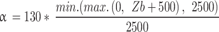
where τ_b represents basal stress, α the basal friction coefficient, N effective pressure, and u_b basal velocity. A spatially varying basal friction coefficient was constructed in three steps. First, the basal friction coefficient α was set proportional to bed elevation  following ref⁵⁸:

2

Second, the basal friction coefficient α was refined in fast flowing areas (≥ 200 m/year) using:

3

with representing satellite-derived ice-flow velocity,  maximum velocity⁴⁹, and a glacier-specific maximum friction coefficient, i.e., 7.8, 8.6, and 11.7 for HPS19, Penguin, and Europa Glacier respectively. Values of  were determined using an inversion method^27,59 that satisfies the best match between modeled and satellite-derived surface velocities⁴⁹. Finally, the minimum basal friction coefficient on land, as well as the friction coefficient below sea level, was set to 10 (m/s)^−1/2.

Calving parameterization

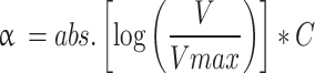
A von Mises calving law was applied to simulate ice-front evolution⁶⁰, where the calving rate is related to tensile stresses within the ice:

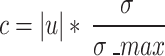4

with the magnitude of the horizontal ice velocity, the von Mises tensile stress, and the maximum stress threshold in the ice. was calibrated to 550 kPa for grounded ice, and 300 kPa for floating ice, by reproducing the present-day ice fronts after a 150-year transient relaxation during which the grounding lines and calving fronts were able to evolve freely. Floating ice thinner than 2 m was set to calve off instantly, independent of the above von Mises parameterization.

Climate forcing

Within our transient Neoglacial simulations, temperature is expressed as anomalies from the 1979–2020 CE mean, and precipitation is expressed as a fraction of the 1979–2020 CE mean. We impose these anomalies onto the 1979–2020 CE monthly mean of temperature and precipitation from the high spatial resolution (0.05°) CAMELS-CL gridded meteorological dataset presented in ref²² to produce the applied Neoglacial temperature and precipitation forcings:

5

6

where _{(1979 – 2020 CE)} and _{(1979 – 2020 CE)} are the monthly mean temperature and precipitation over 1979–2020 CE from ref²², and ∆T_t and ∆P_t are spatially-uniform anomalies. Two different sets of ∆T_twere defined using the proxy-based records of ref^28,29, as well as for ∆P_tby using the records of ref^29,30. Since these records have different temporal resolutions, i.e., 107 ± 47 year (PA; ref²⁸), 147 ± 121 year (TML1; ref³⁰), and 3 ± 1 year (MA1; ref²⁹), they were all resampled at a 100-year resolution and linear interpolation was applied between the resampled data points. Ultimately, we performed four transient simulations using the four combinations of possible climate scenarios (Table 1). The duration of these simulations was limited by the shortest proxy record (4200 years), which was the MA1 temperature record²⁹.

Surface mass balance over the Neoglacial period, and in our future simulations, was computed using a Positive Degree Day (PDD) method⁶¹. PDD factors of 3 and 6 mm ice equivalent °C⁻¹ day⁻¹ were used for snow and ice respectively, in line with previous modeling studies and similar to those observed along the SPI^{18,20,62–65}. The temperature forcing was adjusted using a lapse rate correction of 5.5 °C km⁻¹, following the observations of ref⁶³, to account for changes in ice-surface elevation throughout the simulations. The amount of snow accumulation from total precipitation was computed assuming a normal distribution of the hourly temperature around the monthly means. Precipitation is assumed to fall as rain when the temperature is above 2°C and as snow below 0°C. Between 0 and 2 °C, the snow fraction varies in function of temperature following Bales et al⁴⁵.

Ocean forcing

Basal melting of floating ice was set to linearly increase from 0 at the water surface to 3250 m/year at depths deeper than 100 m, following observations of ocean heat supply in Jorge Montt Fjord, another proglacial fjord located along the northwestern edge of the SPI⁶⁶. We do not simulate horizontal frontal melting explicitly since modern data to constrain this is not available, let alone its evolution over millennial timescales. Instead, we assume that our comparatively low calving stress thresholds on grounded (550 kPa) and floating (300 kPa) ice, and relatively high imposed basal melting of floating ice, include some of the influence from frontal melting on ice-front evolution, following ref⁶¹.

Model initialization

Before running the Neoglacial transient experiments, ice-front positions at the beginning of the Neoglacial period were simulated using a two-step spin up. First, a steady-state spin-up simulation with constant modern climate forcing, i.e., the 1979–2020 CE mean climatology from the CAMELS-CL dataset²², was run for 300 years for ice extent, elevation, and volume to reach a present-day equilibrium. The resulting present-day simulation was in good agreement with the observed grounding-line positions, ice-flow velocities, glacier-surface elevation, and accumulation-area ratio (Supplementary discussion 1). Next, for each Neoglacial forcing scenario, a second spin-up simulation was run for 500 years with constant climate forcing set as the reconstructed climatology at 4.2 kyr b2k for the respective scenarios (#1–4; Table 1). Following this approach, our transient Neoglacial simulations all start from grounding-line positions located in close proximity to their modern locations in both Penguin and Europa fjords (Supplementary Figs. 1, 2, 3, and 4), except for Europa Glacier in simulation #3 which retreated ca. 13 km inland from its present-day grounding line (Supplementary Fig. 3). These ice-front positions at the start of the Neoglacial period are consistent with glacier reconstructions based on geological records from both sides of the SPI^15,31, which show that glacier fronts were located near or within their present margins at the beginning of the Neoglacial period. Nonetheless, to test the impact of the initial grounding-line position on the ice volume simulated during our Neoglacial transient experiments (Fig. 2), we reran all Neoglacial experiments from different grounding-line positions (Supplementary discussion 2).

For the 6.0 kyr simulations discussed in section “Temperature and precipitation forcing over the last 6000 years” (Figs. 3 and 4), model initialization consisted of the same two-step spin-up approach. Here, the second spin-up simulation was run with constant climate forcing set as the reconstructed climatology at 6.0 kyr b2k, i.e., ∆T = + 2.12 °C and ∆P = 101% (Fig. 3; ref^28,30). Doing so, these transient 6.0 kyr simulations again started from grounding-line positions located in close proximity to their modern locations in both Penguin and Europa fjords (Supplementary Fig. 5).

21st century glacier projection experiments

All future simulations presented in Fig. 5 started from the end of the 6.0 kyr simulation (Figs. 3 and 4) which represents the year 2000 CE, and lasted until 2150 CE. We simulated ice-volume changes of the HPS19, Penguin, and Europa glaciers in response to IPCC’s projected 0.8°C (SSP1-2.6), 1.5°C (SSP2-4.5), 2.2°C (SSP3-7.0), and 2.8°C (SSP5-8.5) temperature increase in southern South America by 2081–2100 CE (ref^10,37,38; WGI Interactive Atlas, baseline 1981–2010 CE). For each of these temperature anomalies, we ran simulations using increased precipitation ranging from 0 to 60%, in 10% increments, of its modern amounts following the precipitation projections of Araya-Osses et al. in the Magallanes region by 2081–2100 CE (ref⁹). IPCC’s precipitation projections were not used since their resolution is too low to accurately capture orographic precipitation across the Southern Patagonian Icefield (ref^10,37,38). The advantage of using IPCC’s temperature forecasts, on the other hand, is that they cover the entire region of southern South America and, therefore, encompass both the modeled glaciers and the PA and MA1 proxy-based temperature records. All temperature and precipitation anomalies were applied as spatially-uniform anomalies and prescribed to linearly increase from 0% at 2000 CE to 100% at 2100 CE (in line with our transient Neoglacial simulations), and remained constant at 100% until the end of the sensitivity experiments (2150 CE) for the anomalies applied at 2100 CE to take effect. This approach was specifically chosen, instead of using forcings from general circulation models, to maintain a consistent modeling framework through both our Neoglacial and future simulations. Therefore, all glacier simulations were limited to simulating centennial-scale evolution, which is the temporal resolution of the selected proxy-based reconstructions of Neoglacial temperature and precipitation change (Methods “Climate forcing”). To be clear, all future simulations are sensitivity experiments rather than full projections. We do not aim to reconstruct glacier change over the recent observational period exactly, nor to provide detailed projections of future glacier dynamics and evolution.

Attribution factors AF_P and AF_T

The relative importance of precipitation and temperature in driving Neoglacial ice-volume variations in the 6.0 kyr simulation were calculated using Eq. (7) to (9):

7

with V_n representing ice volume simulated at time n in the 6.0 kyr simulation in response to both temperature and precipitation forcing (Fig. 3), and V_n−1 ice volume 100 years later.

8

with V_{P, n} representing ice volume simulated at time n in the 6.0 kyr simulation with constant temperature forcing (Fig. 3), and V_{P, n−1} ice volume 100 years later.

The final attribution factor of precipitation (AF_P, %) was calculated using Eq. (9):

9

δV_T and AF_T were calculated with Eqs. 8 and 9 but using ice volume simulated with constant precipitation (V_T; Fig. 3).

Supplementary Fig. 9 shows that the denominator of Eq. 9 closely captures the volume changes of the 6.0 kyr simulation (similarity = 97.8%) with a relatively small error (mean absolute error = 0.13 ± 0.25%; root mean square error = 0.28), which highlights the strength of our attribution method. Following this approach, AF_P and AF_T always sum up to 100%, which is consistent with our experimental setup simulating Neoglacial ice-volume changes only in response to variations in air temperature and precipitation (Methods “Climate forcing”). The response of ice volume to variations in ocean forcing was tested using a range of sensitivity experiments (Supplementary discussion 3).

Electronic supplementary material

Below is the link to the electronic supplementary material.

Author contributions

This study was conceived by MT and SB. MT wrote the model script and analyzed the model simulations, with technical advice and scientific support from HÅ and JKC. MT made all figures, and wrote the manuscript with significant contributions from SB, HÅ, and JKC. All authors approved the final version of this manuscript.

Data availability

 The simulations performed in this study made use of the open-source Ice-Sheet and Sea-level System Model (ISSM) and are publicly available at https://issm.jpl.nasa.gov/ (ref.²⁷). The results of our glacier-volume simulations are available in the supplementary spreadsheet.

Declarations

Conflict of interest

The authors hereby declare that the submitted work was not carried out in the presence of any personal, professional or financial relationships that could potentially be construed as a conflict of interest.

References

- 1.Hugonnet, R. et al. Accelerated global glacier mass loss in the early twenty-first century. Nature. 592, 726–731 (2021). [DOI] [PubMed] [Google Scholar]
- 2.Rounce, D. R. et al. Global glacier change in the 21st century: every increase in temperature matters. Sci. (1979). 379, 78–83 (2023). [DOI] [PubMed] [Google Scholar]
- 3.IPCC. IPCC Special Report on the Ocean and Cryosphere in a changing climate. IPCC Intergovernmental Panel Clim. Change. 10.1017/9781009157964 (2019). [Google Scholar]
- 4.Meier, W. J. H., Grießinger, J., Hochreuther, P. & Braun, M. H. An updated multi-temporal glacier inventory for the Patagonian Andes with changes between the little ice age and 2016. Front. Earth Sci. (Lausanne)6, 62. 10.3389/feart.2018.00062 (2018). [Google Scholar]
- 5.Abdel Jaber, W., Rott, H., Floricioiu, D., Wuite, J. & Miranda, N. Heterogeneous spatial and temporal pattern of surface elevation change and mass balance of the Patagonian ice fields between 2000 and 2016. Cryosphere. 13, 2511–2535 (2019). [Google Scholar]
- 6.Davies, B. J. & Glasser, N. F. Accelerating shrinkage of Patagonian glaciers from the little ice age (AD 1870) to 2011. J. Glaciol.58, 1063–1084 (2012). [Google Scholar]
- 7.Bravo, C. et al. Assessing Snow Accumulation patterns and changes on the Patagonian Icefields. Front. Environ. Sci.7, 18 (2019). [Google Scholar]
- 8.Mernild, S. H. et al. The Andes Cordillera. Part I: snow distribution, properties, and trends (1979–2014). Int. J. Climatol.37, 1680–1698 (2017). [Google Scholar]
- 9.Araya-Osses, D., Casanueva, A., Román-Figueroa, C., Uribe, J. M. & Paneque, M. Climate change projections of temperature and precipitation in Chile based on statistical downscaling. Clim. Dyn.54, 4309–4330 (2020). [Google Scholar]
- 10.IPCC. : Climate Change 2023: Synthesis Report. Contribution of Working Groups I, II and III to the Sixth Assessment Report of the Intergovernmental Panel on Climate Change [Core Writing Team, H. Lee and J. Romero (Eds.)]. IPCC, Geneva, Switzerland. (2023) doi: (2023). 10.59327/IPCC/AR6-9789291691647
- 11.Yan, Q., Wei, T. & Zhang, Z. Modeling the climate sensitivity of Patagonian glaciers and their responses to climatic change during the global last glacial maximum. Quat Sci. Rev.288, 107582 (2022). [Google Scholar]
- 12.Hulton, N. R. J., Purves, R. S., McCulloch, R. D., Sugden, D. E. & Bentley, M. J. The last glacial Maximum and deglaciation in southern South America. Quat Sci. Rev.21, 233–241 (2002). [Google Scholar]
- 13.Sugden, D. E., Hulton, N. R. J. & Purves, R. S. Modelling the inception of the Patagonian icesheet. Quatern. Int.95–96, 55–64 (2002). [Google Scholar]
- 14.Bertrand, S. et al. Precipitation as the main driver of Neoglacial fluctuations of Gualas glacier, Northern Patagonian Icefield. Clim. Past. 8, 519–534 (2012). [Google Scholar]
- 15.Troch, M., Bertrand, S., Wellner, J. S., Lange, C. B. & Hughen, K. A. Postglacial fluctuations of western outlet glaciers of the Southern Patagonian Icefield reconstructed from fjord sediments (Chile, 50°S). Quat Sci. Rev.301, 107934 (2023). [Google Scholar]
- 16.Davies, B. J. et al. The evolution of the Patagonian ice sheet from 35 ka to the present day (PATICE). Earth Sci. Rev.204, 103152 (2020). [Google Scholar]
- 17.Bravo, C. et al. Modelled glacier equilibrium line altitudes during the Mid-holocene in the southern mid-latitudes. Clim. Past. 11, 1575–1586 (2015). [Google Scholar]
- 18.Martin, J., Davies, B. J., Jones, R. & Thorndycraft, V. Modelled sensitivity of Monte San Lorenzo ice cap, Patagonian Andes, to past and present climate. Front. Earth Sci. (Lausanne). 10, 1–32 (2022). [Google Scholar]
- 19.Minowa, M., Schaefer, M., Sugiyama, S., Sakakibara, D. & Skvarca, P. Frontal ablation and mass loss of the Patagonian Icefields. Earth Planet. Sci. Lett.561, 116811 (2021). [Google Scholar]
- 20.De Angelis, H. Hypsometry and sensitivity of the mass balance to changes in equilibrium-line altitude: the case of the Southern Patagonia Icefield. J. Glaciol.60, 14–28 (2014). [Google Scholar]
- 21.Dowdeswell, J. A. & Vásquez, M. Submarine landforms in the fjords of southern Chile: implications for glacimarine processes and sedimentation in a mild glacier-influenced environment. Quat Sci. Rev.64, 1–19 (2013). [Google Scholar]
- 22.Alvarez-Garreton, C. et al. The CAMELS-CL dataset: catchment attributes and meteorology for large sample studies-Chile dataset. Hydrol. Earth Syst. Sci.22, 5817–5846 (2018). [Google Scholar]
- 23.Garreaud, R., Lopez, P., Minvielle, M. & Rojas, M. Large-scale control on the Patagonian Climate. J. Clim.26, 215–230 (2013). [Google Scholar]
- 24.Glasser, N. F., Harrison, S., Jansson, K. N., Anderson, K. & Cowley, A. Global sea-level contribution from the Patagonian Icefields since the little ice age maximum. Nat. Geosci.4, 303–307 (2011). [Google Scholar]
- 25.Aniya, M., Skvarca, P., Casassa, G., Sato, H. & Naruse, R. Recent Glacier variations in the Southern Patagonia Icefield, South America. Arct. Alp. Res.29, 1–12 (1997). [Google Scholar]
- 26.Lliboutry, L. Nieves Y Glaciars De Chile, fundamento de glaciologia. Ediciones De La. Universidad De Chile 471 (1956).
- 27.Larour, E., Seroussi, H., Morlighem, M. & Rignot, E. Continental scale, high order, high spatial resolution, ice sheet modeling using the ice sheet System Model (ISSM). J. Geophys. Res. Earth Surf.117, F01022. 10.1029/2011JF002140 (2012). [Google Scholar]
- 28.Massaferro, J. & Larocque-Tobler, I. Using a newly developed chironomid transfer function for reconstructing mean annual air temperature at Lake Potrok Aike, Patagonia, Argentina. Ecol. Indic.24, 201–210 (2013). [Google Scholar]
- 29.Schimpf, D. et al. The significance of chemical, isotopic, and detrital components in three coeval stalagmites from the superhumid southernmost Andes (53°S) as high-resolution palaeo-climate proxies. Quat Sci. Rev.30, 443–459 (2011). [Google Scholar]
- 30.Lamy, F. et al. Holocene changes in the position and intensity of the southern westerly wind belt. Nat. Geosci.3, 695–699 (2010). [Google Scholar]
- 31.Kaplan, M. R. et al. Patagonian and southern South Atlantic view of Holocene climate. Quat Sci. Rev.141, 112–125 (2016). [Google Scholar]
- 32.Fürst, J. J. et al. The foundations of the Patagonian Icefields. Commun. Earth Environ.5, 142 (2024). [Google Scholar]
- 33.Warren, C. & Sugden, D. The Patagonian Icefields: a glaciological review. Arct. Alp. Res.25, 316–331 (1993). [Google Scholar]
- 34.Sagredo, E. A., Rupper, S. & Lowell, T. V. Sensitivities of the equilibrium line altitude to temperature and precipitation changes along the Andes. Quat Res.81, 355–366 (2014). [Google Scholar]
- 35.Cook, K. H., Yang, X., Carter, C. M. & Belcher, B. N. A modeling system for studying climate controls on mountain glaciers with application to the Patagonian Icefields. Clim. Change. 56, 339–367 (2003). [Google Scholar]
- 36.Schaefer, M., Machguth, H., Falvey, M., Casassa, G. & Rignot, E. Quantifying mass balance processes on the Southern Patagonia Icefield. Cryosphere. 9, 25–35 (2015). [Google Scholar]
- 37.Iturbide, M. et al. Repository supporting the implementation of FAIR principles in the IPCC-WG1 Atlas. 10.5281/zenodo.3691645. (2021). https://github.com/IPCC-WG1/Atlas
- 38.Gutiérrez, J. M. et al. Atlas. In Climate Change 2021: The Physical Science Basis. Contribution of Working Group I to the Sixth Assessment Report of the Intergovernmental Panel on Climate Change (eds Masson-Delmotte, V. et al.) (Cambridge University Press, 2021). In Press. Interactive Atlas available from Available from http://interactive-atlas.ipcc.ch/
- 39.Andreassen, L. M., Elvehøy, H., Kjøllmoen, B., Engeset, R. V. & Haakensen, N. Glacier mass-balance and length variation in Norway. Ann. Glaciol. 42, 317–325 (2005). [Google Scholar]
- 40.Hoelzle, M., Haeberli, W., Dischl, M. & Peschke, W. Secular glacier mass balances derived from cumulative glacier length changes. Glob Planet. Change. 36, 295–306 (2003). [Google Scholar]
- 41.Josberger, E. G., Bidlake, W. R., March, R. S. & Kennedy, B. W. Glacier mass-balance fluctuations in the Pacific Northwest and Alaska, USA. Ann. Glaciol. 46, 291–296 (2007). [Google Scholar]
- 42.Foresta, L. et al. Surface elevation change and mass balance of Icelandic ice caps derived from swath mode CryoSat-2 altimetry. Geophys. Res. Lett.43, 12,138–12,145 (2016). [Google Scholar]
- 43.Goodwin, B. P., Mosley-Thompson, E., Wilson, A. B. & Porter, S. E. Roxana Sierra-Hernandez, M. Accumulation variability in the Antarctic Peninsula: the role of large-scale atmospheric oscillations and their interactions*. J. Clim.29, 2579–2596 (2016). [Google Scholar]
- 44.Medley, B. & Thomas, E. R. Increased snowfall over the Antarctic Ice Sheet mitigated twentieth-century sea-level rise. Nat. Clim. Chang.9, 34–39 (2019). [Google Scholar]
- 45.Bales, R. C. et al. Annual accumulation for Greenland updated using ice core data developed during 2000–2006 and analysis of daily coastal meteorological data. J. Geophys. Res. Atmos.114, 1–14 (2009). [Google Scholar]
- 46.Almonacid, L., Pessacg, N., Diaz, B., Bonfili, O. & Peri, P. L. Nueva base de datos reticulada de precipitación para la provincia de Santa Cruz, Argentina. Meteorologica. 46, e007–e007 (2021). [Google Scholar]
- 47.Pfeffer, W. T. et al. The Randolph Glacier Inventory: a globally complete inventory of glaciers. J. Glaciol.60, 537–552 (2014). [Google Scholar]
- 48.RGI Consortium. Randolph glacier inventory 6.0. doi: (2017). 10.7265/N5-RGI-60
- 49.Millan, R., Mouginot, J., Rabatel, A. & Morlighem, M. Ice velocity and thickness of the world’s glaciers. Nat. Geosci.15, 124–129 (2022). [Google Scholar]
- 50.Dias dos Santos, T., Morlighem, M. & Brinkerhoff, D. A new vertically integrated MOno-Layer higher-order (MOLHO) ice flow model. Cryosphere. 16, 179–195 (2022). [Google Scholar]
- 51.Seroussi, H. & Morlighem, M. Representation of basal melting at the grounding line in ice flow models. Cryosphere. 12, 3085–3096 (2018). [Google Scholar]
- 52.Millan, R. et al. Ice thickness and bed elevation of the Northern and Southern Patagonian Icefields. Geophys. Res. Lett.2019GL08248510.1029/2019GL082485 (2019).
- 53.Carrivick, J. L., Davies, B. J., James, W. H. M. & Quincey, D. J. Glasser, N. F. Distributed ice thickness and glacier volume in southern South America. Glob Planet. Change. 146, 122–132 (2016). [Google Scholar]
- 54.Farinotti, D. et al. A consensus estimate for the ice thickness distribution of all glaciers on Earth. Nat. Geosci.12, 168–173 (2019). [Google Scholar]
- 55.Cuffey, K. M. & Paterson, W. S. B. The Physics of Glaciers (Butterworth-Heinemann, 2010).
- 56.Schwikowski, M., Schläppi, M., Santibañez, P., Rivera, A. & Casassa, G. Net accumulation rates derived from ice core stable isotope records of Pío XI glacier, Southern Patagonia Icefield. Cryosphere. 7, 1635–1644 (2013). [Google Scholar]
- 57.Budd, W. F., Keage, P. L. & Blundy, N. A. Empirical studies of ice sliding. J. Glaciol.22, 157–170 (1979). [Google Scholar]
- 58.Åkesson, H., Morlighem, M., Nisancioglu, K. H., Svendsen, J. I. & Mangerud, J. Atmosphere-driven ice sheet mass loss paced by topography: insights from modelling the south-western scandinavian ice sheet. Quat Sci. Rev.195, 32–47 (2018). [Google Scholar]
- 59.Morlighem, M. et al. Spatial patterns of basal drag inferred using control methods from a full-Stokes and simpler models for Pine Island Glacier, West Antarctica. Geophys Res Lett 37, n/a-n/a (2010).
- 60.Morlighem, M. et al. Modeling of Store Gletscher’s calving dynamics, West Greenland, in response to ocean thermal forcing. Geophys. Res. Abstracts (Vol. 21, 43, 2659–2666 (2016). [Google Scholar]
- 61.Cuzzone, J. K., Young, N. E., Morlighem, M., Briner, J. P. & Schlegel, N. J. Simulating the Holocene deglaciation across a marine-terminating portion of southwestern Greenland in response to marine and atmospheric forcings. Cryosphere. 16, 2355–2372 (2022). [Google Scholar]
- 62.Bown, F. et al. Recent ice dynamics and mass balance of Jorge Montt Glacier, Southern Patagonia Icefield. J. Glaciol.65, 732–744 (2019). [Google Scholar]
- 63.Bravo, C. et al. Air temperature characteristics, distribution, and impact on modeled ablation for the South Patagonia Icefield. J. Geophys. Research: Atmos.124, 907–925 (2019). [Google Scholar]
- 64.Rivera, A. University of Bristol,. Mass balance investigations at Glaciar Chico, Southern Patagonia Icefield, Chile. PhD thesis. (2004).
- 65.Stuefer, M., Rott, H. & Skvarca, P. Glaciar Perito Moreno, Patagonia: climate sensitivities and glacier characteristics preceding the 2003/04 and 2005/06 damming events. J. Glaciol.53, 3–16 (2007). [Google Scholar]
- 66.Moffat, C. et al. Seasonal evolution of Ocean Heat Supply and Freshwater Discharge from a rapidly retreating Tidewater Glacier: Jorge Montt, Patagonia. J. Geophys. Res. Oceans. 123, 4200–4223 (2018). [Google Scholar]
Associated Data
This section collects any data citations, data availability statements, or supplementary materials included in this article.
Supplementary Materials
Data Availability Statement