k-Means NANI: an improved clustering algorithm for Molecular Dynamics simulations

Abstract

One of the key challenges of k-means clustering is the seed selection or the initial centroid estimation since the clustering result depends heavily on this choice. Alternatives such as k-means++ have mitigated this limitation by estimating the centroids using an empirical probability distribution. However, with high-dimensional and complex datasets such as those obtained from molecular simulation, k-means++ fails to partition the data in an optimal manner. Furthermore, stochastic elements in all flavors of k-means++ will lead to a lack of reproducibility. K-means N-Ary Natural Initiation (NANI) is presented as an alternative to tackle this challenge by using efficient n-ary comparisons to both identify high-density regions in the data and select a diverse set of initial conformations. Centroids generated from NANI are not only representative of the data and different from one another, helping k-means to partition the data accurately, but also deterministic, providing consistent cluster populations across replicates. From peptide and protein folding molecular simulations, NANI was able to create compact and well-separated clusters as well as accurately find the metastable states that agree with the literature. NANI can cluster diverse datasets and be used as a standalone tool or as part of our MDANCE clustering package.

Graphical Abstract

Introduction

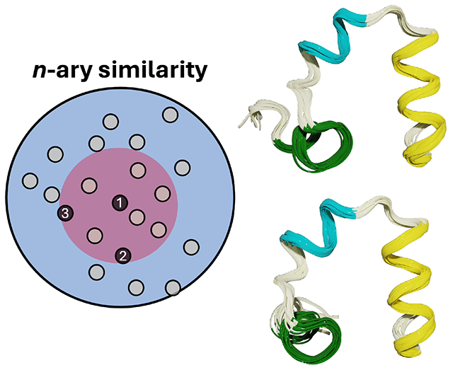
Molecular Dynamics (MD) simulations serve as a computational microscope into intricate biological processes, yet the challenge arises when extending their scope to encompass longer timescales and larger systems. Unfortunately, the post-processing analysis of MD trajectories has struggled to keep pace with this demand, particularly evident in available clustering techniques, which is essential for unraveling protein dynamics and enhanced sampling techniques.¹ Clustering, an unsupervised machine-learning method, identifies patterns within a dataset by organizing similar samples based on a similarity measure.^2,3 When clustering structures obtained from MD simulations there are several metrics that can be used, but it is quite common to use root-mean-square deviation (RMSD) as the clustering metric.^4–6 The RMSD is typically used in pair-wise manner, where the RMSD of a conformation is calculated to every other conformation in the ensemble, leading to O(N²) scaling of the clustering calculation. There are also many clustering algorithms, but choosing one often involves a stark trade-off: conventional algorithms such as k-means^7,8 prove efficient but fall short in identifying subtle metastable states, whereas more robust methods like density-based clustering (e.g. DBSCAN,^9,10 density peak¹¹) incur significant computational overhead.^2,12,13 In this contribution, we present the first module of our Molecular Dynamics Analysis with N-ary Clustering Ensembles (MDANCE) software package based on n-ary similarity (that is, using the notion of comparing multiple objects at the same time).^14–20 Overall, MDANCE is aimed to provide great flexibility, new clustering algorithms, and novel tools to process the clustering results and to assess the overall quality of the clustering process. In the first installment of MDANCE, we will be introducing k-means N-ary Natural Initiation (NANI), an initialization method for k-means.

K-means is widely known to be the most popular clustering algorithm in the community for its straightforward approach. It was first proposed by Stuart Lloyd in 1957 and formalized by James MacQueen in 1967; now, it has become a central component of unsupervised learning for pattern recognition and data science. The input for k-means requires two parameters: the number of clusters and an initial estimate of the centroids. Beginning with initial centroid estimates, the algorithm proceeds by assigning each data point to the nearest centroid and recalculating the centroids for each cluster iteratively until convergence, in which the computed centroids remain the same, and data points stay within their respective clusters. When applied to large datasets from Molecular Dynamics, it proves to be efficient as it has a time complexity of O(k × N × i), k for the number of clusters, n for the number of points, and i for the number of iterations.²¹

Despite its efficiency, the K-means algorithm can struggle to identify metastable states due to one or more of the following issues: poor selection of the number of clusters (k), problems with the initial centroid estimation, and the clustering of non-convex shapes. The selection of k is a required input parameter for the algorithm. However, determining k can be challenging given the multidimensional and complex nature of most datasets, so the number of metastable states is often determined a priori.²² A larger k can result in finer partitioning of the data, which can identify some of the metastable states; however, this risks the accuracy of the cluster population and transition probabilities between clusters.²³ The initial centroid estimation is also important because subsequent points are assigned based on these estimates. Therefore, many different initialization methods (e.g. k-means++^24,25) were proposed to predict the best centroids for initialization (See Theory Section). However, all the existing centroid estimation algorithms are stochastic, which makes it challenging to assess the validity of the results. Lastly, k-means is not designed to identify non-convex cluster shapes since it is a partitioning cluster algorithm; the resulting cluster shapes tend to be uniform and globular and will usually not adapt arbitrary cluster shape.^26–29 Another algorithm similar to k-means is k-medoids,³⁰ which is similar to K-means except that the data points are assigned to the nearest medoid. Therefore, pairwise comparisons are performed to determine the similarity between every point to determine the least dissimilar object, making the algorithm less sensitive to outliers.² Due to the pairwise comparisons and inefficiency with high-dimensional data, it has a time complexity of O(k × N² × i).³¹ Since it is not as efficient as k-means, k-medoids will not be investigated in this study.

N-Ary Natural Initiation (NANI) is our proposed initialization technique for k-means with advantages of being fully deterministic, selecting the most diverse structures, and including a pipeline to determine the most optimal number of clusters. The main advantages of NANI are its efficient scaling, deterministic character, and ability to identify more compact and well-defined clusters over realistic MD simulations. Because all the initialization methods available are stochastic, NANI is an attractive option for producing reproducible results. A critical component of the NANI algorithm is diversity selection, which will be elaborated in the Theory Section. The extended similarity-based diversity selection can select a more diverse set of structures from a trajectory than k-means and hierarchical agglomerative clustering in O(N) time complexity.¹⁸ Lastly, the choice of number of clusters is not trivial, especially in a multidimensional dataset, where the user might even need knowledge about the system to make this decision.³² A pipeline has been established to make this decision to require minimal presumptions. A process involves screening through a range of k’s, and utilizing clustering quality metrics to determine the most optimal k. Through these additions, k-means clustering can obtain robust results even for multidimensional and complex datasets.

Theory

Tools

Alignment.

The most intuitive representation of an MD trajectory is the spatial coordinates of atoms in the trajectory. However, this can be challenging because configurations need to be aligned to some reference(s) to compensate for the effect of rotations and translations during a simulation and the decision of what reference(s) to align to can impact the data analysis significantly.^33,34 Here, we explore two possibilities to handle the alignment: the traditional alignment to a single reference conformation, and the Kronecker version of the alignment proposed by McCullagh et al.³⁵ Typically (at least for coordinates from MD trajectories), the optimal rotation for minimizing the differences between two sets of coordinate vectors in Cartesian space has used either the procedure of Kabsch³⁶ or a quaternion-based method.^37,38 The Kronecker method is somewhat different, consisting of a global alignment where weight is distributed according to the variance of the atoms’ coordinates. Specifically, the Mahalanobis distance³⁵ of the total set of conformations is minimized. However, after this, the distance between the individual conformations is measured using standard techniques. When using Cartesian coordinates the first step in the clustering process is to perform this alignment in order to set the position and orientation of every conformation in a univocal reference frame. This is critical to any k-means variant, since we need to be able to rank distances obtained in the same footing. For example, let us say that we have two cluster centroids, A and B, and a conformation X that we need to assign to one of these clusters. To do this it is paramount that the distances X-A and X-B are consistent with each other, that is, X, A, and B must retain their relative positions when calculating their relative separations. This is lost if we align X to A to calculate their separation, and then align X to B to perform the same calculation. Any iterative alignment procedure will lead to distances calculated in two unrelated reference frames, so there is no clear way to rank the separation of X from the tentative cluster centroids. This is why the alignment should only be performed once before starting the k-means clustering. It is also important to notice that one can bypass the need to perform the alignment if instead of Cartesian we use a complete set of internal coordinates. (That is, an arbitrary set of internal coordinates is not on itself enough to overcome this issue, but carefully selected internal coordinates provide a univocal frame of reference in which to perform the clustering.) In the SI we include a short proof-of-principle example of NANI based on internal coordinates to highlight the broad applicability of our method (Fig. S12).

N-ary Similarity.

Traditionally, we quantify the similarity of objects using pairwise functions, that is, taking two objects at a time. The problem with this approach is that when we want to study N objects we need to compute the similarity between every possible pair of objects in the set, which demands O(N²) computational effort. We have recently shown how it is possible to define n-ary functions to quantify similarity and differences (either through extended or instant similarity indices),^14,15,17 and that can take an arbitrary number of inputs at the same time and evaluate their similarity with a much more attractive O(N) scaling. While most of the applications of these metrics have been in cheminformatics and drug design problems, here we use some of the basic principles to study conformational ensembles of different biomolecules. For instance, a fundamental condition required by all n-ary indices is that the objects to be compared must be represented by vectors with the same length (e.g., with the same number of components). This means that we can arrange all the items to be compared in a 2D array (e.g., the ”representation matrix”), with each row representing an element to be analyzed. Then, the key insight that allows the n-ary indices to turn this into an O(N) problem is realizing that we just need to generate a vector containing the sums of the elements of each column of the representation matrix (or, at most in the case of real continuous inputs, also the vector containing the sum of the squares of each element in a given column). The vector of column sums is all that is needed to quantify how related are all the elements in the set. There are several recipes to do this, depending on the type of similarity index that one desires to use (the original paper on extended similarity included dozens of examples on how to generate n-ary indices^14,15). In particular, in the case of MD simulations, it is customary to use the RMSD to calculate how separated the two conformations are. In the next section, we show how to obtain an n-ary measure that closely resembles the RMSD behavior, yet allows comparing N structures in O(N).

Mean Squared Deviation.

For a system with M atoms and D coordinates, let us denote the ith frame by $F^{(i)}$. Then, the RMSD between the ith and jth frames, $F^{(i)}=\left[q_1^{(i)},q_2^{(i)},\dots ,q_D^{(i)}\right]$,$F^{(j)}=\left[q_1^{(j)},q_2^{(j)},\dots ,q_D^{(j)}\right]$ (where $q_k^{(i)}$ represents the kth coordinate of the ith frame), is calculated as:

$$RMSD(i,j)=\sqrt{\frac{\sum _{k=1}^{k=D}{(q_k^{(i)}-q_k^{(j)})}^2}{M}}$$ (1)

Similarly, we can define the Mean Squared Deviation (MSD) between two frames as:

$$MSD(i,j)=\frac{\sum _{k=1}^{k=D}{\left(q_k^{(i)}-q_k^{(j)}\right)}^2}{M}$$ (2)

The key difference between these two magnitudes comes when calculating their average over N > 2 frames. For instance, in the case of the RMSD, it is clear that this will demand O(N²) scaling:

$$\begin{gathered} \langle RMSD\rangle =\frac{1}{N^2}\sum _{i=1}^N\sum _{j=1}^{N}RMSD(i,j) \\ =\frac{1}{N^2}\sum _{i=1}^N\sum _{j=1}^N\sqrt{\frac{\sum _{k=1}^{k=D}{\left(q_k^{(i)}-q_k^{(j)}\right)}^2}{M}} \end{gathered}$$ (3)

However, this is not the case for the MSD:

$$\begin{gathered} \langle MSD\rangle =\frac{1}{N^2}\sum _{i=1}^N\sum _{j=1}^{N}MSD(i,j) \\ =\frac{1}{M{N}^2}\sum _{i=1}^N\sum _{j=1}^N\sum _{k=1}^{k=D}{\left(q_k^{(i)}-q_k^{(j)}\right)}^2 \\ =\frac{2}{M{N}^2}\sum _{k=1}^{k=D}\left\{N\sum _{i=1}^N{\left(q_k^{(i)}\right)}^2-{\left(\sum _{i=1}^N{q}_k^{(i)}\right)}^2\right\} \end{gathered}$$ (4)

Notice that in the last equation, we only need $\sum _{i=1}^N{\left(q_k^{(i)}\right)}^2$ and $\sum _{i=1}^N{q}_k^{(i)}$, and since they both scale as O(N), the overall MSD calculation has a much more attractive linear cost (while also bypassing the cumbersome square root calculation). As noted in the previous sub-section, this is the critical step in the calculation of any n-ary index, and hence the critical difference between the RMSD and the MSD.

Complementary Similarity.

Calculating the medoid of a set scales in O(N²), or O(N log N) at best. However, using complementary similarity, we can identify the medoid in O(N).²⁰ The complementary similarity is based on the idea of the n-ary similarity; it calculates the n-ary similarity of a set without a given element. Therefore, the medoid will correspond to the highest complementary MSD (cMSD) as the set is more dissimilar overall without the most representative member. Likewise, outliers will correspond to low cMSD, since removing them contributes to making the set more compact. The complementary similarity will determine the ranking of how representative or outlier a member of the set is, from most representative (medoid) to most outlier-like.

Diversity Selection.

Another useful tool in n-ary similarity is sampling representative structures from a set. It picks the first points using complementary similarity to find the medoid. It then picks the most dissimilar point from the selected point(s) at every iteration. That is, at any given point, we pick the point that minimizes the overall similarity of the selected set, as measured by an n-ary function.

Clustering

K-means is a partitioning clustering algorithm that assigns points to the closest centroid. It iterates by recalculating the centroid and reassigning points. Other than the determination of the number of clusters, initial centroid prediction is critical as the clustering is susceptible to modifications in the labeling with different centroid estimations. Therefore, a diverse set of initial centroids is required for better results than random initialization. Some of the available initialization methods (illustrated in Figs. 1 and 2), including our proposed NANI, are presented below:

Figure 1:

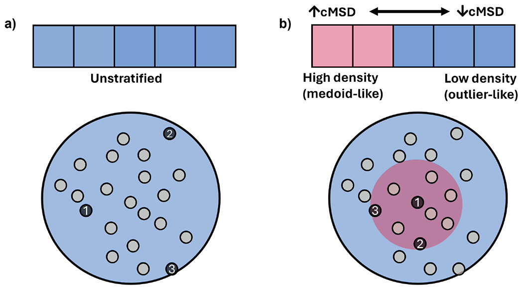
(a) Initialization scheme for all k-means++ flavors. (b) Initialization scheme for k-means++ NANI.

Figure 2: Four centroid selection algorithms for k-means initialization.

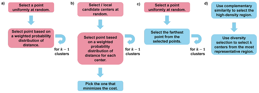
(a) Vanilla k-means++ (b) Greedy k-means++ (c) CPPTRAJ (d) NANI. Pink boxes indicate stochastic steps and blue boxes indicate fully deterministic steps. After these initialization setups, assignment and update cycles are performed until convergence.

Vanilla k-means++ is the original version of k-means++.²⁴ The algorithm begins by initially picking a random point from the set. It will then pick the next point using a weighted probability distribution of distance from the selected point and will favor selecting the point with the maximum distance from the selected point. It will continue for k number of clusters. Since the algorithm has stochastic elements, results will vary every time.

Greedy k-means++ follows the same algorithm as its vanilla version, except it runs multiple local trials of initialization and picks the best one for k-means clustering. The greedy version can perform better than the vanilla variant, but this is not guaranteed to be always the case^24,39 and it is the default setting for initializing k-means in scikit-learn.⁴⁰ This algorithm provides good results for simple and well-separated systems. However, its limitation is apparent in noisier data (See Fig. 3).

Figure 3:

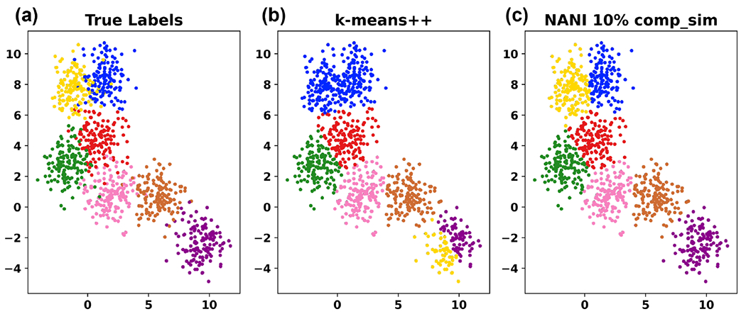
k-means NANI on a sample 2D data with a known number of clusters (7). A different color represents a different cluster label. (a) True Labels. (b) k-means clustering with centroids initialized by k-means++ and took 12 iterations to converge resulting in 0.85 V-measure score. (c) k-means clustering with centroids initialized by k-means NANI and took 11 iterations to converge resulting in 0.80 V-measure score.

CPPTRAJ Initialization starts from a random point and selects the farthest point from the selected points.⁴¹ It then iterates for k number of clusters.

N-Ary Natural Initiation (NANI) NANI first uses the medoid algorithm to stratify the data into high-density regions and then performs a diversity selection (Max_nDis, ECS_MeDiv) to pick well-separated centroids.¹⁵ The diversity selection starts with the medoid of the dataset. It iterates the data to find the object with the lowest similarity between the candidate and the existing set of centroids. This procedure is inspired by k-means++, but with the key difference that the first point is chosen in a completely deterministic way. MDANCE includes two NANI variants: div_select is the closest one to the standard k-means++, in the sense that the last k − 1 centroids are chosen from all the remaining points in the set. On the other hand, the comp_sim version of NANI is even more efficient, since we use all the complementary similarity values to stratify the data, and then do the diversity selection of the remaining k – 1 centers only over a high-density fraction of the initial points. A key insight here is that using the n-ary complementary similarity algorithm to stratify the data ensures that this algorithm retains the attractive scaling of traditional k-means.

It is important to remark that all the methods discussed in this section only differ on how they select the initial k points. That is, after this selection, they all proceed in the same way, alternating assignment and update steps. In the former, points are assigned to their closest centroid (hence why it is paramount that all the distances are calculated in an univocal reference frame, as noted in the alignment section above). Then, centroids are updated to reflect the new assignments. These two steps are alternated until some convergence criterion is reached.

Finally, the bulk of this paper is dedicated to the comparison of NANI with other k-means alternatives. However, due to the popularity of Hierarchical Agglomerative Clustering (HAC) methods in the MD community, we include a short comparison of NANI and average and complete HAC in the SI. The highlight of this comparison is the difference in computational resources needed to perform these analyses. While the HAC study of the HP35 simulation described in the next section took more than 2 days, NANI only required 85 seconds to complete this task.

Systems and Software

2D Datasets.

The model 2D data was obtained from scikit-learn single-labeled generated dataset. The blob disk, nine diamonds, and ellipses were extracted from Veenman et al, Salvador et al, and Bandyopadhyay et al, respectively.^42–46

β-Heptapeptide

The topology and trajectory files correspond to publicly available data and were assessed through GitHub.^47,48 The atom selection follows Daura et al,⁴⁹ Lys2 to Asp11, with N, Cα, C, O, and H atoms. The terminal and side chain residues were ignored to minimize noise in the clustering. The single-reference alignment was done after aligning to the 1000^th frame. Also, we performed the Kronecker alignment as a comparison.

β-Hairpin

This system was adapted from a stabilized β-hairpin system proposed here.⁵⁰ Orn-8 was substituted with Lys-8 due to lack of ornithine parameters in the force field; this substitution was tested previously⁵¹ and was found to have minimal impact on the conformational stability. Subsequent MD simulations indicated that the peptide was often kinetically trapped due to strong salt-bridging interactions between Arg-1 and Glu-4; for the purpose of facilitating ensemble convergence, we introduced an R1Q substitution. Neutral capping groups (ACE, NHE) also were introduced at the termini to further reduce the possibility of strong electrostatic traps. This modified system was then relaxed to stabilize the initial structure before eight independent MD simulations of ~9 μs each were generated at 420K (~70 μs total). The ensuing ensemble was very diverse, with backbone RMSD’s ranging from under 1 angstrom to over 10 angstrom and featuring ~11,000 folding and unfolding events. ~65,000 equally spaced coordinate sets were extracted for analysis. All clustering on this system used the backbone atoms (Cα, C, and N) and all frames were aligned to the 1000^th frame that was extracted.

HP35.

Analysis was performed on a 305 μs, all-atom simulation of Nle/Nle mutant of the C-terminal subdomain of the Villin headpiece (also known as HP35) from D. E. Shaw Research.⁵² This simulation was conducted at a temperature of 360 K and consists of 1.52 million frames with a frame separation of 200 ps. All frames in the simulation were aligned to the 5000^th frame in the simulations and frames before the 5000^th frame were discarded as a relaxation phase. The backbone atom selection encompassed the following atoms: N of residue 1, CA, C, N of residues 2 to 34, and N from residue 35; this selection is consistent with previous studies of HP35. A sieve was applied on every 20^th frame, resulting in a total of ~89,000 frames for clustering.

NuG2.

An analysis was conducted on a dataset comprising four independent all-atom simulations of NuG2, a mutant variant of Protein G. The simulations, with a cumulative duration of 1.15 milliseconds (5.78 million frames with a frame separation of 200 ps), were conducted at a temperature of 350 K and carried out by D. E. Shaw Research.⁵³ All frames in the simulation were aligned to the 5000^th frame in the simulations and frames before the 5000^th frame were discarded as a relaxation phase. The atom selection encompasses the backbone atoms (CA, C, and N) of residues 1 to 56; this selection is consistent with previous studies of NuG2. A sieve was applied on every 65^th frame, resulting in a total of ~76,000 frames for clustering.

MDANCE.

The NANI code is available as one of two modules in the MDANCE package. MDANCE contains basic functionality in a Behind The Scenes (BTS) module that handles I/O functions, interfacing with packages like AMBER⁵⁴ and MDAnalysis,^55,56 along with several alignment options. The NANI module handles the initial seed selection procedure for both the comp_sim and div_select variants, but it can easily be modified to include other selection criteria. While the applications in this paper are centered around the use of the MSD as n-ary difference measure, MDANCE gives the user the option to use from other n-ary indices, like extended versions of popular cheminformatic metrics like Tanimoto, Russel-Rao, etc. The MDANCE GitHub repository can be found here: https://github.com/mqcomplab/MDANCE.

Results and discussion

2D Datasets

Clustering evaluation metrics assess the quality of the resulting clusters. Clustering evaluation metrics are separated into internal and external measures; internal measures do not use ground-truth labels, whereas external measures require ground-truth labels. Internal measures are primarily used for complex data where a ground-truth label is unavailable. Several indicators were studied to identify the most optimum metric for identifying the number of clusters in a dataset.

V-measure score⁵⁷ calculates how accurately the clustering labels match the ground truth based on two criteria—homogeneity and completeness. The dataset is divided into classes and after clustering, the algorithm separates the dataset into clusters. Homogeneity measures the purity of the cluster if all the members in a cluster contain only members with the same class label. Completeness measures if all the members with the same class label are in one cluster. These two criteria will calculate a V-measure score between 0 to 1. A V-measure closer to 1 indicates greater accuracy to the ground truth labels. This metric is an external measure, which requires ground truth labels as input. Therefore, the V-measure will not be used for simulation data since there are no known cluster labels.

Calinski-Harabasz index⁵⁸ (CH, also known as variance ratio criterion) is a clustering evaluation metric that quantifies the separation between clusters and the compactness within clusters. CH is a ratio of between-cluster dispersion and within-cluster dispersion. Between-cluster dispersion is a sum of squares between each cluster centroid and the centroid of the dataset. Within-cluster dispersion is the sum of squares between samples in the data and their respective cluster centroids. A high CH value indicates well-separated clusters. CH index is an internal measure, which is solely based on the dataset and clustering results and does not use ground-truth labels in the calculation, which makes it a candidate for a metric for quantifying simulation data.

Both the Calinski-Harabasz index (CH) and Silhouette score are popular cluster evaluation metrics for measuring cluster quality in the community.^1,32 Silhouette score⁵⁹ is also an internal clustering measure and calculates intra- and inter-cluster distances. For every data point, the algorithm calculates the average distance to all other points in that cluster (a) and also calculates the average distance to all the points in the nearest cluster (b). The score is calculates using silhouette score = (b – a)/ max(a, b). Values range between −1 to 1, with −1 meaning the point is clustered poorly, values close to 0 meaning the point is close to a border with another cluster, and 1 meaning the point is well-clustered. Because silhouette score typically requires a pairwise matrix, it is O(N²) and the slowest out of all mentioned metrics.

Average mean squared deviation (MSD) only takes into account the clustering labels and the coordinates and determines how compact clusters are, in which a lower MSD would be a tighter cluster. Similar to RMSD, mean squared deviation determines the similarity between frames. Average MSD calculates the similarity of clusters using the n-ary framework. This metric is the least computationally intensive out of all the clustering quality metrics.

Similar to CH and Silhouette score, the Davies-Bouldin index (DBI)⁶⁰ is an internal clustering measure and quantifies similarity within and between clusters. DBI is a ratio between intra-cluster and inter-cluster similarity. The intra-cluster similarity is the average distance between points in a cluster and the centroid of the cluster. The inter-cluster similarity is the distance between the cluster centroids. A lower DBI value indicates clusters that are far apart and tightly packed.

Not only is k-means NANI (comp_sim and div_select) both a deterministic seed selector, but it also results in more compact and well-defined clusters with linear scaling comparable to k-means++. In our 2D results, k-means NANI was able to correctly identify the clusters of noisy data (See Fig. 3) because it begins with the medoid and only selects from high-density regions. Fig. 4 shows measures of the robustness of different clustering techniques using average MSD, CH index, DBI index, number of iterations, and V-measure score. div_select is similar to the initialization used in CPPTRAJ because both choose the farthest point from the already selected points. Since div_select only sometimes surpasses the other variants and usually takes more iterations compared to comp_sim, only comp_sim will be investigated in the simulation data. On the other hand, comp_sim surpassed k-means++ variants in all clustering metrics, further motivating its use as a seed selector for k-means clustering. Therefore, from now on, whenever we refer to NANI, we are implicitly referring to the comp_sim variant.

Figure 4:

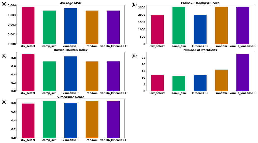
Cluster characteristics of different seed selectors on a sample 2D data from Fig. 3. (a) Average MSD of the clusters using different seed selectors (↓). (b) Calinski-Harabasz index (↑). (c) Davies-Bouldin index (↑). (d) Number of iterations (↓). (e) V-measure score (↑).

Application to Peptide Systems

A key part of our clustering pipeline is the incorporation of the previously discussed indicators to quantify the quality of the final clustering. This is critical to identify the optimum number of clusters in the data. In all cases, we performed a scan over different values of k, which is especially necessary when analyzing realistic MD simulations. Then, different clustering quality metrics will be explored to identify the most ideal metrics for the clustering pipeline hereinafter.

The Calinski-Harabasz index (CH) measures how well-separated clusters are and the trend for CH is that a larger index would indicate an optimal number of clusters. However, all the graphs exhibit the same behavior as shown in Fig. 5 with changing different variables (systems, alignment method, initialization technique). It seems unlikely that two clusters would be the most optimal number of clusters in every case; however, CH tends to favor a small number of clusters due to its bias for convex shapes. Overall, the behavior of NANI and the two k-means++ variants is very similar, with the CPPTRAJ algorithm consistently resulting in lower CH values. Also note the variations on the CPPTRAJ and k-means++ results, especially for the β-hairpin and HP35 systems. As far as the quality of the clusters goes, there does not seem to be an increase in the separation of clusters when we use the Kronecker alignment (with the β-heptapeptide and β-hairpin even showing a better behavior for the single reference alignment).

Figure 5:

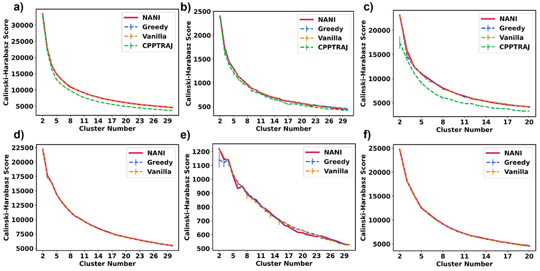
Calinski-Harabasz index (y-axis) vs. cluster number (x-axis) of different seed selectors applied on three peptide systems. Error bars represent the standard deviation over three replicates. (a) β-hairpin single-reference aligned (b) β-heptapeptide single-reference aligned (c) HP35 single-reference aligned (d) β-hairpin Kronecker aligned (e) β-heptapeptide Kronecker aligned (f) HP35 Kronecker aligned

The Silhouette score is another metric to measure similarity within and between clusters. A similar issue with this metric is that it favors a smaller number of clusters due to its bias for convex clusters. A bigger issue with the Silhouette and CH indices is that their change from one k value to another does not seem to be a good indicator of the optimum number of clusters in the set. This is particularly evident in the case of CH, with the values just monotonically increasing with decreasing k values. A similar pattern is followed by the Silhouette score, which is more evident for the β-hairpin and HP35 cases, as shown in Fig. 6. There, the score just tends to either remain essentially constant over a range of k values or just tends to increase. The β-heptapeptide system highlights a particularly pathological Silhouette behavior, with the single reference and Kronecker alignments presenting totally opposed trends for this score. Given that the β-hairpin simulations were conducted at the highest temperatures, and thus are expected to boast higher conformational plasticity, this seems to indicate that the silhouette score is not appropriate to identify the optimum k values for these simulations.

Figure 6:

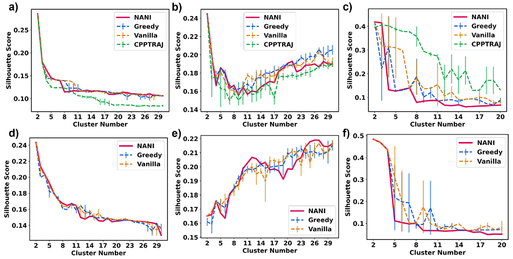
Average Silhouette score (y-axis) vs Number of clusters (x-axis) of different seed selectors applied on three peptide systems. Error bars represent the standard deviation over three replicates. (a) β-hairpin single-reference aligned (b) β-heptapeptide single-reference aligned (c) HP35 single-reference aligned (d) β-hairpin Kronecker aligned (e) β-heptapeptide Kronecker aligned (f) HP35 Kronecker aligned

The average mean squared deviation (MSD) would indicate how compact a cluster is. MSD follows the trend of a decreasing concave-up shape due to the nature of an increasingly more dissimilar cluster as it grows and a more similar cluster as it is smaller. Just like for the CH index, the MSD values tend to change monotonically, so at first sight, they do not seem suitable to identify optimum k values, as shown in Fig. 7. However, interestingly, in several cases, we could correlate the changes in the slope of the MSD graphs with the behavior of optimum k values of other indicators, chiefly, the Davies-Bouldin index analyzed in the next section. When NANI was applied to the Molecular Dynamics trajectory, the compactness was greater than that of k-means++ as demonstrated by the average MSD values.

Figure 7:

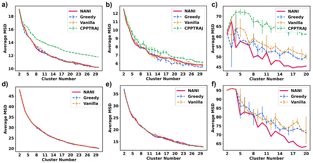
Average mean squared deviation (y-axis) vs Number of clusters (x-axis) of different seed selectors applied on three peptide systems. Error bars represent the standard deviation over three replicates. (a) β-hairpin single-reference aligned (b) β-heptapeptide single-reference aligned (c) HP35 single-reference aligned (d) β-hairpin Kronecker aligned (e) β-heptapeptide Kronecker aligned (f) HP35 Kronecker aligned

Davies-Bouldin index (DBI) is the metric that works the best for the most number of systems. DBI measures both the intercluster and intracluster distance and a lower DBI would indicate an optimal number of clusters. This is usually the case for simple systems, but with high-dimensional and complex datasets this can sometimes be misleading because DBI tends to favor a small number of clusters, the minimum value is not always the optimum number. Moreover, for most indicators designed to quantify the quality of the clustering, it can be argued that their local behavior is more important than their absolute values. (This has been recently emphasized by Hocky, McCullagh, et al.⁶¹) While this is in principle true for any of these indices (and, in a sense, can be seen as the rationalization behind the ”elbow method”), it is more useful in the case of the DBI. Once again, the almost perfectly monotonic behavior of the CH index renders this approach useless. On the other hand, the quasi-constant behavior of the Silhouette index over intervals of k values, coupled with an almost monotonic increase for some systems, also makes this a relatively difficult criterion to adapt in that case. Therefore, we introduced another criterion for measuring the optimal DBI—the maximum second derivative DBI. The maximum 2^nd derivative of DBI with respect to the number of clusters is the local minimum of the two steepest slopes, which can often indicate the most optimal value before it rises and drops back to global minima, which is due to DBI’s bias for convex clusters. In other words, the 2^nd derivative criterion allows users to distinguish ”unusually stable” k values, while tending to be more robust towards the bias for particular cluster shapes. From Fig. 8, DBI proves to be a more robust metric compared to CH and silhouette score as the topology of the graph is different for different systems, while also remaining easily quantifiable, and without presenting obvious biases towards a particular range of k values. Comparing the DBI for the different initialization methods, the CPPTRAJ method gives the highest DBI would indicate a weaker initialization method than the other three since it is farthest from the desired low values. However, both vanilla and greedy k-means++ methods were not as robust as NANI as there were great fluctuations in the DBI values between runs. Since all methods contain elements of probability and randomness, they are not as robust as the deterministic NANI methods because they will give a different optimal number of clusters every time the user executes the methods. This pathological behavior is shown in Table 1, where we present the results of three replicates of Greedy, Vanilla, and CPPTRAJ k-means. Notice that for all the peptide systems, and independently of if the optimum k is selected with the absolute value or the 2^nd derivative of DBI, different runs tend to give different values for the optimum value of k. NANI not only gives the DBI values in every replicate, but it also gives DBI values of the same quality, if not better in several instances, than those of the k-means++ variants. It is important to highlight that the lack of reproducibility of the other k-means implementations goes beyond ”merely” identifying different numbers of clusters. The relative importance of certain conformations and the main representatives of each cluster is also altered from one run to the other, as shown in Fig. S13 in the SI section.

Figure 8:

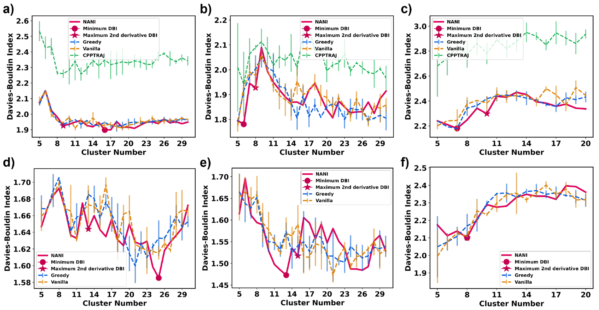
Davies–Bouldin index (y-axis) vs Number of clusters (x-axis) of different seed selectors applied on three peptide systems. Error bars represent the standard deviation over three replicates. (a) β-hairpin single-reference aligned (b) β-heptapeptide single-reference aligned (c) HP35 single-reference aligned (d) β-hairpin Kronecker aligned (e) β-heptapeptide Kronecker aligned (f) HP35 Kronecker aligned

Table 1:

Optimum number of clusters over for the studied systems, as determined by running three replicas of the Greedy, Vanilla, and CPPTRAJ algorithms. Top: k values determined from the absolute minimum of the DBI index. Bottom: k values determined from the 2^nd derivative of the DBI index. In all cases, only k values bigger or equal to 5 were considered.

Algorithm/System	β-heptapeptide	β-hairpin	HP35
Absolute DBI values
NANI	6/6/6	16/16/16	7/7/7
Greedy	15/23/17	20/18/12	7/7/7
Vanilla	5/27/5	18/15/11	7/5/7
CPPTRAJ	5/6/30	15/11/9	5/12/5
2nd Derivative of DBI values
NANI	8/8/8	9/9/9	10/10/10
Greedy	8/15/17	20/12/12	7/17/7
Vanilla	14/8/13	11/11/11	7/18/7
CPPTRAJ	20/6/15	15/8/6	8/19/10

To further highlight NANI’s performance, we dissected the HP35 simulations in more detail, given the recent interest in this system as a benchmark for other clustering methods. In the application to HP35, the number of clusters was determined to be seven using single-reference alignment and calculated using NANI as the seed selector. In the overlaps (See Fig. 9, it shows that NANI was able to identify seven metastable states of HP35 with cluster populations consistent with a previous study (using more computationally demanding clustering methods) in which six metastable states were reduced to a four-state model consisting of a native state N (53% of the population), a native-like state N’ (14%), an intermediate state I (18%), and an unfolded state U (15%).³⁵ As shown in Fig. 10, NANI obtains similar populations for N (66%), N’ (8%), I (9%), and U (17%). (We assigned all the structures in each NANI cluster to the same state.) The results are consistent for both the ”condensed” version of the results (corresponding to k = 4), or the optimal configuration with k = 7. N’ is the partial unfolding of helix 3.^35,62 In all cases, the N’ conformation was found to be the least populated. N1 and N2 are two conformations in the folded state (N) except for the orientation of helix 1 (See Fig. 11), but both are highly tight clusters, representative of the native folded structure of HP35; overall, the N state is the most populated cluster. Three clusters corresponded to the unfolded state (U), with uncoiling observed in U1, U2, and U3. U2 has a unique orientation of helix 1 and 3 with both turning away from helix 2. U1 has a more defined structure in helix 3 than in U3. The intermediate structure is observed to have decreased variance from the unfolded states, with defined structures in all three helices but not yet completely folded.

Figure 9:

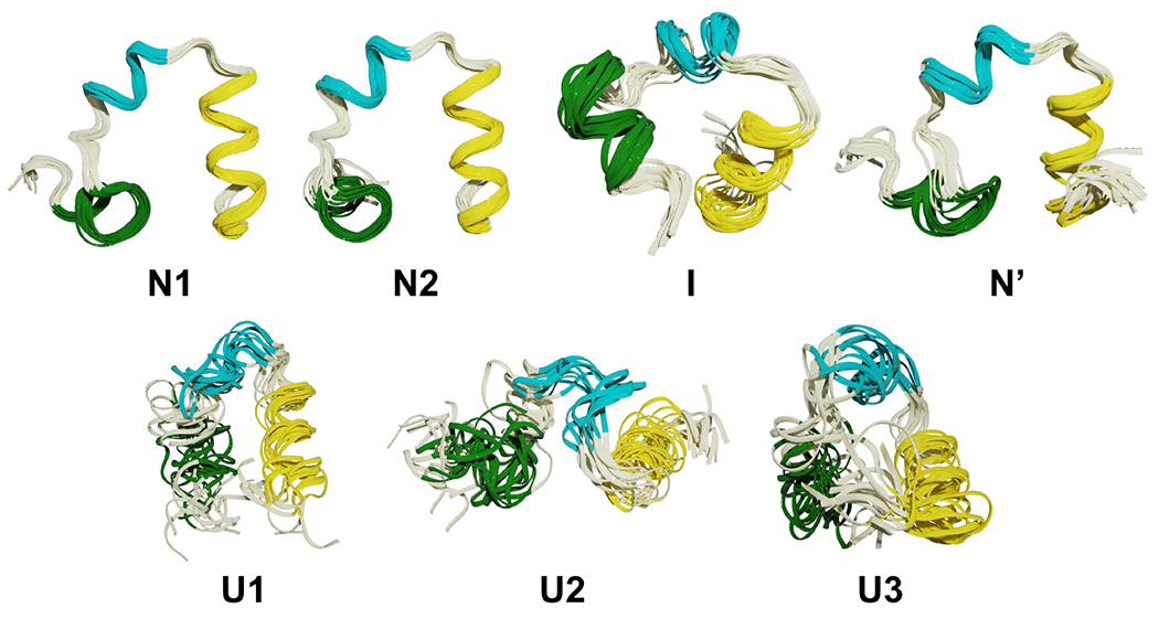
Structural overlaps for HP35 in four states: folded (N), partially folded (N’), intermediate (I), and unfolded (U). Helix 1, 2, and 3 are in green, cyan, and yellow, respectively.

Figure 10:

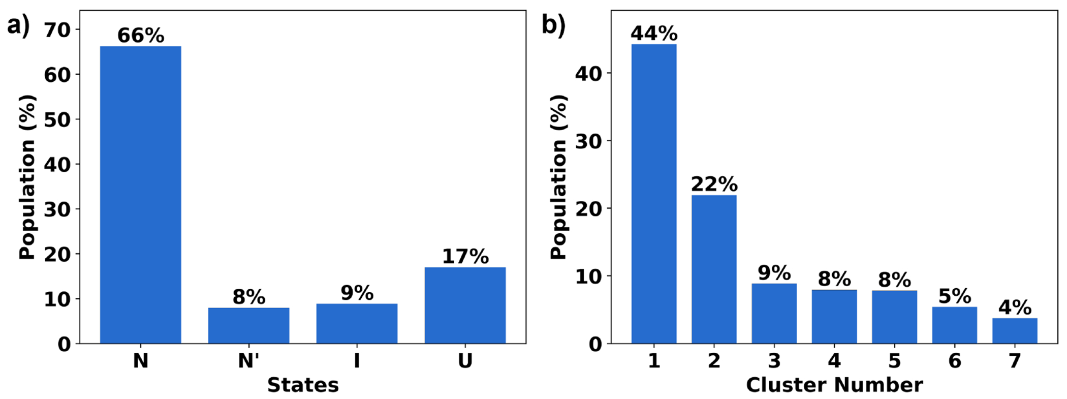
(a) Cluster population for HP35 in four states: folded (N), partially folded (N’), intermediate (I), and unfolded (U). (b) Individual cluster population.

Figure 11:

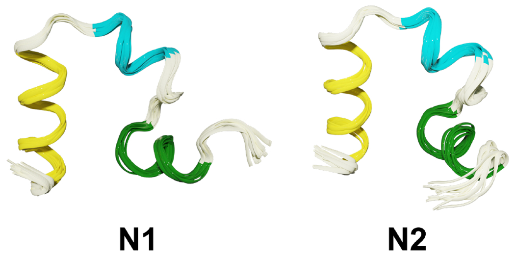
Another view of the structural overlaps for HP35 in two folded (N) states.

Kronecker alignment has some limitations compared to single-reference alignment (See Fig. S10) because it is unable to recognize the N’ state. This is surprising since this alignment was able to find this conformational basin when combined with Shape-GMM clustering. This seems to indicate that for a simple method, like k-means NANI, the single reference alignment might be a more convenient starting point.

NuG2

NuG2 has a complex protein-folding mechanism as it has two β-sheets and an α-helix, and can follow two different pathways to fold.⁶³ Given the results of the previous section, the clustering for NuG2 only uses the single-reference alignment. The same trend from the peptide section is also observed in NuG2 clustering: NANI can generate compact and well-defined clusters as shown in the lower MSD and DBI values (See Fig. 12). The results from all flavors of the k-means++ predecessors fluctuated greatly between replicates, significantly altering the number of clusters per run. Once again, the standard CPPTRAJ k-means implementation resulted in the highest MSD and DBI values and the lowest CH values, while also showing a significant variance in the final results, like the k-means++ flavors. The number of clusters was determined to be fifteen calculated using NANI as the seed selector. The folded structure was the predominant cluster at 45%, eight intermediate structures were identified at 39%, three pre-folded structures were found at 10%, and lastly, three unfolded structures were observed at 5% (See Fig. 13). It is remarkable that an algorithm as simple and efficient as NANI was able to find metastable states corresponding to both folding pathways. In our previous studies on this system, we showed that traditional hierarchical agglomerative clustering (HAC) methods failed to identify several intermediate conformations along the folding process.²⁰ Only a variant of HAC that used an n-ary linkage criterion (and was based on a contact map representation of NuG2) was able to distinguish between these states. However, as with every HAC algorithm, this (at best) scales as O(N²), so it is markedly less efficient than k-means NANI. The dominant folded structure revealed well-overlapped structures in the cluster, with the lowest variances. In all the intermediate, a partial unfolding of the β3/4 strands is observed; due to this unfolding, many different conformations were adapted by β3/4 (See Fig. 14). In all the pre-folded states, all β3/4 and the α-helix were partially unfolded; moreover, β1/2 was also observed to have greater variance in the structure compared to the structures in the intermediate states. Unfolded states uncovered a complete unfolding of all three secondary structures in the protein.

Figure 12:

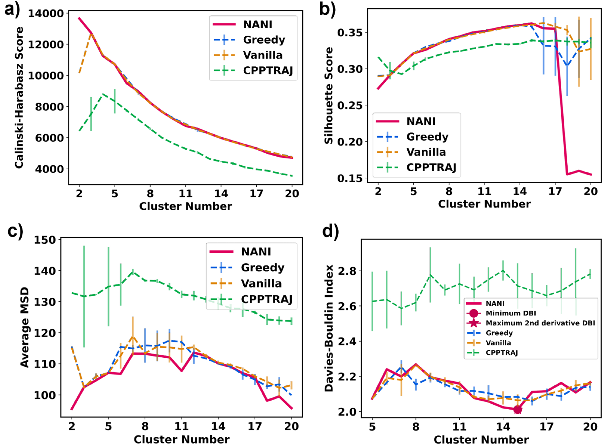
Indicators of different seed selectors applied on NuG2. Error bars represent the standard deviation over three replicates. All use the single-reference alignment. (a) Calinski-Harabasz index (b) Silhouette score (c) Average mean squared deviation (d) Davies–Bouldin index

Figure 13:

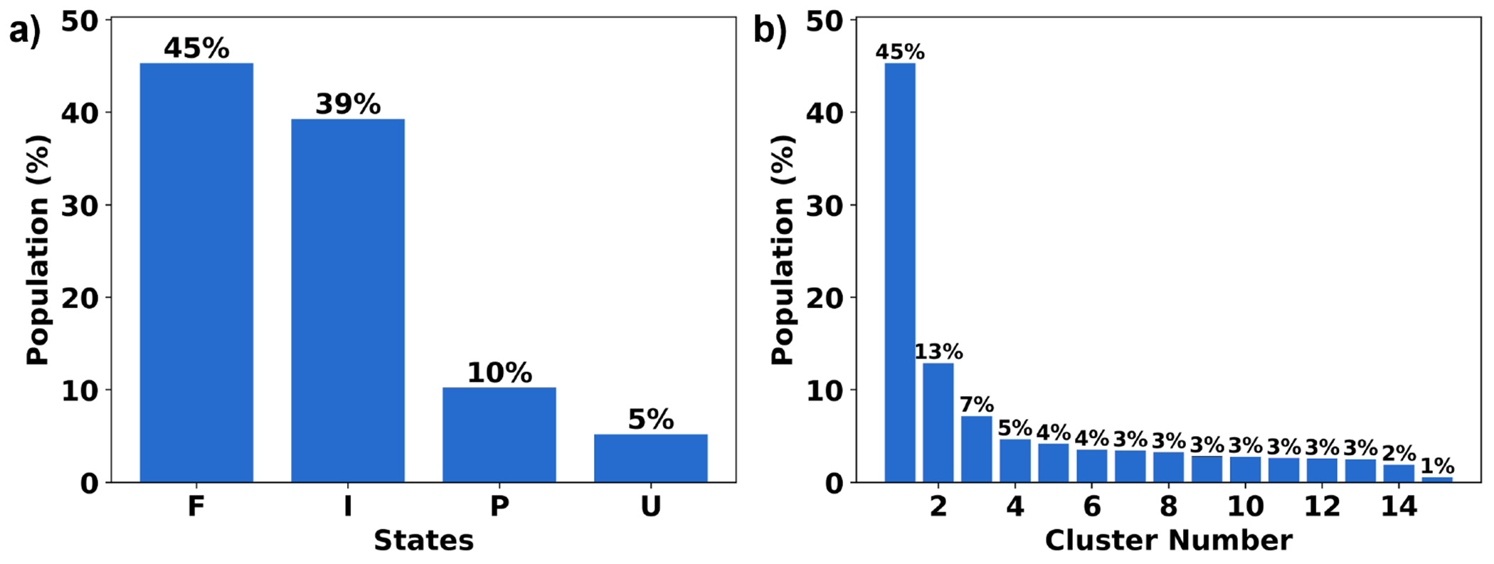
(a) Cluster population for NuG2 in four states: folded (F), intermediate (I), pre-folded (P), and unfolded (U). (b) Individual cluster population.

Figure 14:

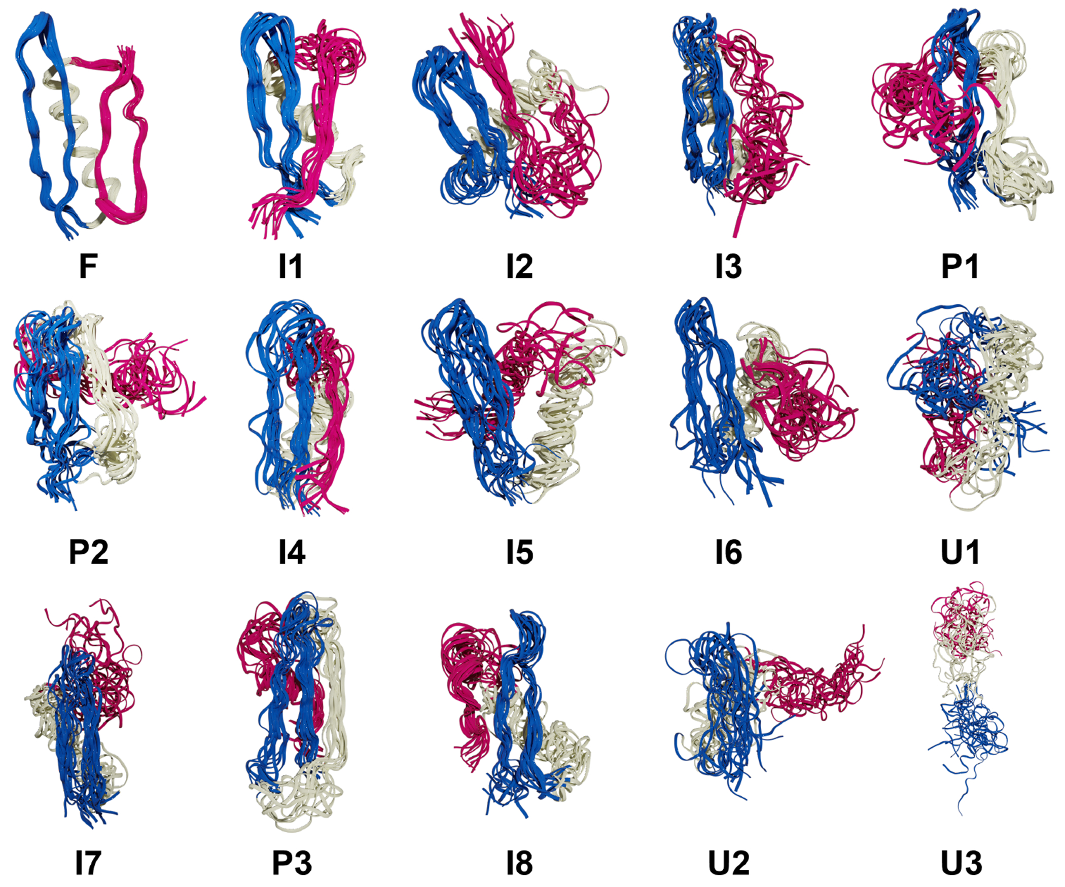
Structural overlaps for NuG2 in four states: folded (F), intermediate (I), pre-folded (P), and unfolded (U). β1 and β2 strands are colored blue, the helix is colored white, and β3 and β4 strands are colored pink.

Conclusion

NANI is a robust seed selector for k-means that surpasses most publicly available seed selectors such as k-means++ and the seed selector for CPPTRAJ k-means. Its advantage comes from its reproducibility as a deterministic algorithm, which gives the same optimal number of clusters and cluster population at each run. Furthermore, as shown in the lower DBI and average MSD values, it excels at creating tight and well-defined clusters. When applied to model 2D systems, the comp_sim version of NANI (the one that chooses centroids only from previously stratified data) highlighted the cause of the potential issues found in the traditional k-means++ and CPPTRAJ implementations. That is, the diversity-picking algorithms applied to the whole set of points tend to select initial centroids in the boundary of the set, which are typically low-density regions. Hence, even though it is expected that the final centroids are well-separated, they will also be found in regions with a higher density of frames. This is more evident with the standard CPPTRAJ implementation, which is the one that most aggressively tries to maximize the separation between initial centroids, which seems to cause the optimization of the k-means objective function to be stuck into local minima where the final centroids are not optimally distributed. Both k-means++ initializations tend to correct this behavior by using a probabilistic diversity exploration mechanism. In this way, they de-emphasize the role of very distant points and allow themselves to potentially select guesses in the high-density zones. However, this introduces further randomness in the final results. NANI combines the best of these worlds, by trying to maximize the diversity of the initial centroids but limiting the exploration of a pre-stratified subset of the data, that is more likely to contain only regions with a higher density of points. The study of even simple peptide systems showcased one of the key issues of any clustering study: identifying the optimum number of clusters in the data. We considered several popular clustering evaluation metrics for doing so, including the CH index and Silhouette score. The former showed an almost perfect monotonically increasing tendency with decreasing number of clusters, while the latter was either virtually constant over ranges of k values, or also monotonically increasing (or, in the case of the β-hairpin, its results varied wildly depending on the alignment). On the other hand, the DBI clustering evaluation metric proved to be more amenable to interpretation. While it can also show a marked bias towards very small k values, we found two ways to work around this issue. First, the overall non-monotonic behavior of this index means that if one restricts the scan of k values to not include very small k values (k = 2, 3, 4), it is possible to identify a physically meaningful number of clusters. Moreover, if one decides to follow the local behavior of the DBI index, instead of its absolute value, and uses the 2^nd derivative as a way to gauge the relative stability of the k values, it is also possible to determine the optimum k values. Finally, on the matter of preferred k values, while the absolute values of the average MSD cannot be used for this purpose, we noted that the 2^nd derivative of the MSD values correlates with the ideal k values found using the DBI index. Given the ease of calculation of the MSD compared to the DBI, it seems reasonable to perform an MSD scan analysis over extended ranges of k’s, and then only perform the DBI calculations for the k values identified through the MSD analysis. This seems like a convenient strategy to aid in speeding up the post-processing of the clustering results, which we will explore in a forthcoming contribution.

The MD simulations also served to highlight some of the key advantages of NANI. Above all, NANI offers a reproducibility that is not attainable with the other k-means algorithms. While the probabilistic nature of the k-means++ methods does not have a great impact on the final results for model 2D systems, this quickly changes even for simple MD simulations. The CH, MSD, and Silhouette scores profiles for both k-means++ flavors showed marked differences from one run to the other, and this was particularly evident for the DBI. This is especially concerning since, as discussed before, DBI seems to be the more robust at the time of determining the ideal k for the given simulation, i.e. different k-means++ runs can lead to different answers about the number of clusters present in the data. The CPPTRAJ k-means also shows great variability, but it is also accompanied by overall lower quality indicators of the considered scores. This indicates that even if we were to use some deterministic criterion to choose the initial centroid in the CPPTRAJ algorithm, choosing the remaining k – 1 initial centers doing a diversity screening over all the frames will lead to picking centers in very low-populated regions in the data, which is a sub-optimal choice. (This agrees with the comparatively sub-par performance of the div_select algorithm on the model 2D systems.) NANI then offers a fully deterministic alternative, with overall performance on par (if not better) than the k-means++ alternatives. We also studied two different alignment paradigms: the traditional single-reference, and the Hocky and McCullagh Kronecker alignments.³⁵ We observed that single-reference tends to produce more compact clusters (as measured by the average MSD), while the Kronecker method tends to result in better-separated clusters (as quantified by the DBI). In general, both alignment methods have strengths and weaknesses, and it is certainly desirable to explore their relative performance when compared in conjunction with other clustering algorithms. In the present case, we tend to slightly favor the combination of single-reference with k-means because this was the combination that allowed identifying the previously reported metastable states for the HP35 and NuG2 systems. It is reassuring to see how NANI was able to not only find the previously identified N, N’, I, and U states of HP35 but also with relative populations in good agreement with those found by more complex (and time-consuming) algorithms. The same success was found for the NuG2 protein, with NANI being able to identify several metastable states across multiple folding pathways that were absent even in the (markedly) less efficient hierarchical studies.

This study introduced NANI as the first installment of our MDANCE clustering package, which can be used as a standalone software or part of our clustering package. Aside from introducing novel clustering algorithms, a pipeline for clustering analysis is also available for determining the most optimal number of clusters for the dataset. In forthcoming contributions, we will expand on the functionality of MDANCE, and we will add more clustering algorithms to this package based on the use of n-ary similarity and difference functions.

References

- (1).Shao J; Tanner SW; Thompson N; Cheatham TE Clustering Molecular Dynamics Trajectories: 1. Characterizing the Performance of Different Clustering Algorithms. Journal of Chemical Theory and Computation 2007, 3, 2312–2334. [DOI] [PubMed] [Google Scholar]
- (2).Glielmo A; Husic BE; Rodriguez A; Clementi C; Noé F; Laio A Unsupervised Learning Methods for Molecular Simulation Data. Chemical Reviews 2021, 121, 9722–9758. [DOI] [PMC free article] [PubMed] [Google Scholar]
- (3).Abramyan TM; Snyder JA; Thyparambil AA; Stuart SJ; Latour RA Cluster analysis of molecular simulation trajectories for systems where both conformation and orientation of the sampled states are important. Journal of Computational Chemistry 2016, 37, 1973–1982. [DOI] [PMC free article] [PubMed] [Google Scholar]
- (4).De Paris R; Quevedo CV; Ruiz DD; Norberto de Souza O; Barros RC Clustering Molecular Dynamics Trajectories for Optimizing Docking Experiments. Computational Intelligence and Neuroscience 2015, 2015, 916240. [DOI] [PMC free article] [PubMed] [Google Scholar]
- (5).Landon MR; Amaro RE; Baron R; Ngan CH; Ozonoff D; Andrew McCammon J; Vajda S Novel Druggable Hot Spots in Avian Influenza Neuraminidase H5N1 Revealed by Computational Solvent Mapping of a Reduced and Representative Receptor Ensemble. Chemical Biology & Drug Design 2008, 71, 106–116. [DOI] [PMC free article] [PubMed] [Google Scholar]
- (6).Troyer JM; Cohen FE Protein conformational landscapes: Energy minimization and clustering of a long molecular dynamics trajectory. Proteins: Structure, Function, and Bioinformatics 1995, 23, 97–110. [DOI] [PubMed] [Google Scholar]
- (7).MacQueen JB Some methods for classification and analysis of multivariate observations. Proceedings of the 5th berkeley symposium on mathematical statistics and probability, volume 1: Statistics. 1967; pp 281–297. [Google Scholar]
- (8).Jain AK; Dubes RC Algorithms for clustering data; Prentice-Hall, Inc.: USA, 1988. [Google Scholar]
- (9).Ester M; Kriegel H-P; Sander J; Xu X A density-based algorithm for discovering clusters in large spatial databases with noise. Proceedings of the second international conference on knowledge discovery and data mining. 1996; pp 226–231. [Google Scholar]
- (10).Schubert E; Sander J; Ester M; Kriegel HP; Xu X DBSCAN Revisited, Revisited: Why and How You Should (Still) Use DBSCAN. ACM Transactions on Database Systems 2017, 42, 1–21. [Google Scholar]
- (11).Rodriguez A; Laio A Clustering by fast search and find of density peaks. Science 2014, 344, 1492–1496. [DOI] [PubMed] [Google Scholar]
- (12).Lemke O; Keller BG Density-based cluster algorithms for the identification of core sets. The Journal of Chemical Physics 2016, 145, 164104. [DOI] [PubMed] [Google Scholar]
- (13).Lemke O; Keller B Common Nearest Neighbor Clustering—A Benchmark. Algorithms 2018, 11, 19. [Google Scholar]
- (14).Miranda-Quintana RA; Bajusz D; Rácz A; Héberger K Extended similarity indices: the benefits of comparing more than two objects simultaneously. Part 1: Theory and characteristics†. Journal of Cheminformatics 2021, 13, 32. [DOI] [PMC free article] [PubMed] [Google Scholar]
- (15).Miranda-Quintana RA; Rácz A; Bajusz D; Héberger K Extended similarity indices: the benefits of comparing more than two objects simultaneously. Part 2: speed, consistency, diversity selection. Journal of Cheminformatics 2021, 13, 33. [DOI] [PMC free article] [PubMed] [Google Scholar]
- (16).Rácz A; Dunn TB; Bajusz D; Kim TD; Miranda-Quintana RA; Héberger K Extended continuous similarity indices: theory and application for QSAR descriptor selection. Journal of Computer-Aided Molecular Design 2022, 36, 157–173. [DOI] [PubMed] [Google Scholar]
- (17).López-Pérez K; Kim TD; Miranda-Quintana RA iSIM: instant similarity. Digital Discovery 2024, 10.1039.D4DD00041B. [DOI] [PMC free article] [PubMed] [Google Scholar]
- (18).Rácz A; Mihalovits LM; Bajusz D; Héberger K; Miranda-Quintana RA Molecular Dynamics Simulations and Diversity Selection by Extended Continuous Similarity Indices. Journal of Chemical Information and Modeling 2022, 62, 3415–3425. [DOI] [PMC free article] [PubMed] [Google Scholar]
- (19).Rácz A; Bajusz D; Héberger K Life beyond the Tanimoto coefficient: similarity measures for interaction fingerprints. Journal of Cheminformatics 2018, 10, 48. [DOI] [PMC free article] [PubMed] [Google Scholar]
- (20).Chang L; Perez A; Miranda-Quintana RA Improving the analysis of biological ensembles through extended similarity measures. Physical Chemistry Chemical Physics 2022, 24, 444–451. [DOI] [PubMed] [Google Scholar]
- (21).Xu D; Tian Y A Comprehensive Survey of Clustering Algorithms. Annals of Data Science 2015, 2, 165–193. [Google Scholar]
- (22).Bremer PL; De Boer D; Alvarado W; Martinez X; Sorin EJ Overcoming the Heuristic Nature of k -Means Clustering: Identification and Characterization of Binding Modes from Simulations of Molecular Recognition Complexes. Journal of Chemical Information and Modeling 2020, 60, 3081–3092. [DOI] [PubMed] [Google Scholar]
- (23).Sittel F; Stock G Perspective: Identification of collective variables and metastable states of protein dynamics. The Journal of Chemical Physics 2018, 149, 150901. [DOI] [PubMed] [Google Scholar]
- (24).Arthur D; Vassilvitskii S k-means++: the advantages of careful seeding. Proceedings of the eighteenth annual ACM-SIAM symposium on discrete algorithms. USA, 2007; pp 1027–1035. [Google Scholar]
- (25).Wang S; Chang T-H; Cui Y; Pang J-S Clustering by orthogonal NMF model and non-convex penalty optimization. IEEE Transactions on Signal Processing 2021, 69, 5273–5288. [Google Scholar]
- (26).Boomija MD; Phil M Comparison of partition based clustering algorithms. Journal of Computer Applications 2008, 1, 18–21. [Google Scholar]
- (27).Wang H; Gao J; Xie M.-g. Clustering of Trajectories using Non-Parametric Conformal DBSCAN Algorithm. 2022 21st ACM/IEEE International Conference on Information Processing in Sensor Networks (IPSN). Milano, Italy, 2022; pp 451–462. [Google Scholar]
- (28).Bhargav S A Review of Clustering Methods forming Non-Convex clusters with, Missing and Noisy Data. International Journal of Computer Sciences and Engineering 2016, 4 [Google Scholar]
- (29).Nguyen CH; Mamitsuka H On Convex Clustering Solutions. 2021; http://arxiv.org/abs/2105.08348, Accessed on 2024-02-21.
- (30).Kaufman L; Rousseeuw PJ Finding groups in data: An introduction to cluster analysis; John Wiley, 1990. [Google Scholar]
- (31).Schubert E; Rousseeuw PJ Faster k-Medoids Clustering: Improving the PAM, CLARA, and CLARANS Algorithms. Similarity Search and Applications. Cham, 2019; pp 171–187. [Google Scholar]
- (32).Melvin RL; Godwin RC; Xiao J; Thompson WG; Berenhaut KS; Salsbury FR Uncovering Large-Scale Conformational Change in Molecular Dynamics without Prior Knowledge. Journal of Chemical Theory and Computation 2016, 12, 6130–6146. [DOI] [PMC free article] [PubMed] [Google Scholar]
- (33).Theobald DL; Wuttke DS Accurate Structural Correlations from Maximum Likelihood Superpositions. PLOS Computational Biology 2008, 4, e43. [DOI] [PMC free article] [PubMed] [Google Scholar]
- (34).Theobald DL; Wuttke DS THESEUS: maximum likelihood superpositioning and analysis of macromolecular structures. Bioinformatics 2006, 22, 2171–2172. [DOI] [PMC free article] [PubMed] [Google Scholar]
- (35).Klem H; Hocky GM; McCullagh M Size-and-Shape Space Gaussian Mixture Models for Structural Clustering of Molecular Dynamics Trajectories. Journal of Chemical Theory and Computation 2022, 18, 3218–3230. [DOI] [PMC free article] [PubMed] [Google Scholar]
- (36).Kabsch W A discussion of the solution for the best rotation to relate two sets of vectors. Acta Crystallographica Section A: Foundations of Crystallography 1978, 34, 827–828. [Google Scholar]
- (37).Coutsias EA; Seok C; Dill KA Using quaternions to calculate RMSD. Journal of Computational Chemistry 2004, 25, 1849–1857. [DOI] [PubMed] [Google Scholar]
- (38).Theobald DL Rapid calculation of RMSDs using a quaternion-based characteristic polynomial. Acta Crystallographica Section A Foundations of Crystallography 2005, 61, 478–480. [DOI] [PubMed] [Google Scholar]
- (39).Grunau C; Özüdoǧru AA; Rozhoň V; Tětek J A Nearly Tight Analysis of Greedy k-means++. 2022; http://arxiv.org/abs/2207.07949, Accessed on 2024-01-24.
- (40).Pedregosa F; Varoquaux G; Gramfort A; Michel V; Thirion B; Grisel O; Blondel M; Prettenhofer P; Weiss R; Dubourg V et al. Scikit-learn: Machine learning in Python. Journal of Machine Learning Research 2011, 12, 2825–2830. [Google Scholar]
- (41).Roe DR; Cheatham TE PTRAJ and CPPTRAJ: Software for Processing and Analysis of Molecular Dynamics Trajectory Data. Journal of Chemical Theory and Computation 2013, 9, 3084–3095. [DOI] [PubMed] [Google Scholar]
- (42).Veenman C; Reinders M; Backer E A maximum variance cluster algorithm. IEEE Transactions on Pattern Analysis and Machine Intelligence 2002, 24, 1273–1280. [Google Scholar]
- (43).Salvador S; Chan P Determining the number of clusters/segments in hierarchical clustering/segmentation algorithms. 16th IEEE International Conference on Tools with Artificial Intelligence. Boca Raton, FL, USA, 2004; pp 576–584. [Google Scholar]
- (44).Bandyopadhyay S; Pal S Classification and Learning Using Genetic Algorithms: Applications in Bioinformatics and Web Intelligence; 2007. [Google Scholar]
- (45).Bandyopadhyay S; Maulik U Nonparametric genetic clustering: comparison of validity indices. IEEE Transactions on Systems, Man and Cybernetics, Part C (Applications and Reviews) 2001, 31, 120–125. [Google Scholar]
- (46).Bandyopadhyay S; Maulik U Genetic clustering for automatic evolution of clusters and application to image classification. Pattern Recognition 2002, 35, 1197–1208. [Google Scholar]
- (47).González-Alemán R; Hernández-Castillo D; Caballero J; Montero-Cabrera LA Quality Threshold Clustering of Molecular Dynamics: A Word of Caution. Journal of Chemical Information and Modeling 2020, 60, 467–472. [DOI] [PubMed] [Google Scholar]
- (48).González-Alemán R Graph-based approach to the quality threshold clustering of molecular dynamics. 2022; https://github.com/LQCT/BitQT, Accessed on 2024-02-21. [DOI] [PubMed]
- (49).Daura X; Conchillo-Solé O On Quality Thresholds for the Clustering of Molecular Structures. Journal of Chemical Information and Modeling 2022, 62, 5738–5745. [DOI] [PMC free article] [PubMed] [Google Scholar]
- (50).Stanger HE; Gellman SH Rules for Antiparallel Beta-Sheet Design: d-Pro-Gly Is Superior to l-Asn-Gly for Beta-Hairpin Nucleation1. Journal of the American Chemical Society 1998, 120, 4236–4237. [Google Scholar]
- (51).Syud FA; Espinosa JF; Gellman SH NMR-Based Quantification of Beta-Sheet Populations in Aqueous Solution through Use of Reference Peptides for the Folded and Unfolded States. Journal of the American Chemical Society 1999, 121, 11577–11578. [Google Scholar]
- (52).Piana S; Lindorff-Larsen K; Shaw DE Protein folding kinetics and thermodynamics from atomistic simulation. Proceedings of the National Academy of Sciences 2012, 109, 17845–17850. [DOI] [PMC free article] [PubMed] [Google Scholar]
- (53).Lindorff-Larsen K; Piana S; Dror RO; Shaw DE How Fast-Folding Proteins Fold. Science 2011, 334 , 517–520. [DOI] [PubMed] [Google Scholar]
- (54).Case D; Belfon K; Ben-Shalom I; Brozell S; Cerutti D; Cheatham ITE; Cruzeiro V; Darden T; Duke R; Giambasu G et al. Amber 2020; University of California, San Francisco, 2020. [Google Scholar]
- (55).Gowers R; Linke M; Barnoud J; Reddy T; Melo M; Seyler S; Domański J; Dotson D; Buchoux S; Kenney I et al. MDAnalysis: A Python Package for the Rapid Analysis of Molecular Dynamics Simulations. Austin, Texas, 2016; pp 98–105. [Google Scholar]
- (56).Michaud-Agrawal N; Denning EJ; Woolf TB; Beckstein O MDAnalysis: A toolkit for the analysis of molecular dynamics simulations. Journal of Computational Chemistry 2011, 32, 2319–2327. [DOI] [PMC free article] [PubMed] [Google Scholar]
- (57).Rosenberg A; Hirschberg J V-measure: A conditional entropy-based external cluster evaluation measure. Proceedings of the 2007 joint conference on empirical methods in natural language processing and computational natural language learning (EMNLP-CoNLL). 2007; pp 410–420. [Google Scholar]
- (58).Caliński T; Harabasz J A dendrite method for cluster analysis. Communications in Statistics 1974, 3, 1–27. [Google Scholar]
- (59).Rousseeuw PJ Silhouettes: A graphical aid to the interpretation and validation of cluster analysis. Journal of Computational and Applied Mathematics 1987, 20, 53–65. [Google Scholar]
- (60).Davies DL; Bouldin DW A Cluster Separation Measure. IEEE Transactions on Pattern Analysis and Machine Intelligence 1979, PAMI-1, 224–227. [PubMed] [Google Scholar]
- (61).Sasmal S; Pal T; Hocky GM; McCullagh M Quantifying unbiased conformational ensembles from biased simulations using ShapeGMM. 2024; 10.1101/2024.01.22.576692, Accessed on 2024-02-21. [DOI] [PMC free article] [PubMed]
- (62).Chang H-W; Bacallado S; Pande VS; Carlsson GE Persistent Topology and Metastable State in Conformational Dynamics. PLoS ONE 2013, 8, e58699. [DOI] [PMC free article] [PubMed] [Google Scholar]
- (63).Mitsutake A; Takano H Folding pathways of NuG2—a designed mutant of protein G—using relaxation mode analysis. The Journal of Chemical Physics 2019, 151, 044117. [DOI] [PubMed] [Google Scholar]
Associated Data
This section collects any data citations, data availability statements, or supplementary materials included in this article.