Thermal performance prediction of a V-trough solar water heater with a modified twisted tape using ANFIS, G.L.R., R.T. and SVM models of machine learning

Abstract

Four distinct neural models were used to evaluate the efficiency of a V-trough solar water heater (VTSWH) equipped with square-cut twisted tape (SCTT) and V-cut twisted tape (VCTT) at two different twist ratios, 3 and 5. The objective of this study was the use of ANFIS (Adaptive Neuro-Fuzzy Inference System), G.L.R. (Generalised linear regression), R.T. (Regression tree), and SVM (Support Vector Machine). A total of 162 data sets were acquired for these models through a variety of trials. Outdoor experiments were done using a twist ratio of Y = 3 and Y = 5, using both SCTT and VCTT. The models included eight distinct variables: ambient temperature, water mass flow rate, water intake temperature, water exit temperature, absorber plate temperature, tube temperature, solar intensity, and twist ratio. The dependent variables in this study are the Nusselt number (Nu), friction factor (FF), and efficiency (η). 130 datasets were chosen for training purposes, while 32 were used for testing. Using the ANFIS, G.L.R., R.T., and SVM techniques, the correlation coefficient (R²) values for Nusselt number were 0.9990, 0.9961, 0.9562, and 0.9280 for friction factor 0.9966, 0.9683, 0.9810, and 0.9560, and for efficiency 0.9997, 0.9976, 0.9845, and 0.9614, respectively. Comparing all models shows that ANFIS is the most effective of the four strategies studied. The ANFIS model outperformed the other models regarding Nu, FF, and η, with RMSE values of 0.0805, 0.0.0004, and 0.4534. According to the above data, the VTSWH thermal performance predicted using the ANFIS approach has the highest accuracy.

Introduction

As a result of increasing affluence and population, these nations will continue to rely heavily on fossil fuels to meet their growing energy needs. But because the earth’s stockpile of fossil fuels is limited, we must look to new energy sources to satisfy our needs. Clean, renewable energy will become more and more crucial as fossil fuels become scarce. Solar Energy is one of the most prevalent and eco-friendly renewable energy. Solar energy usage may be done both actively and passively. The use of passive solar energy doesn’t require any mechanical machinery. However, in the case of active solar energy utilisation, mechanical equipment is needed to convert solar energy into various forms of energy. Devices that use passive solar energy include S.W.H.s. S.W.H.s perform ineffectively because of their limited heating capacity, poor thermal conductivity, and poor convective heat transfer coefficient between the absorber plate and the water flowing through the pipe. As a result, a passive strategy is often adopted in residential and rural settings. Several improvement methods, including absorber plate coating, different types of glazing glass, and thermal insulation, increase the solar water heater’s efficiency. The twist tape technique improves heat transfer performance among the different approaches. Many studies are being conducted to enhance heat exchanger thermal performance using twist tape inserts. However, some research still needs to be completed to enhance the thermal performance of solar water heaters.

Kumar and Prasad¹examined the use of twisted helical tape to improve the heat transfer performance of an S.W.H. with forced circulation. Saravanan et al^2–5. improved the thermal performance of VTSWH in both active and passive modes by using several kinds of twisted tape. Murugan et al^6–8. improved S.W.H. performance using corrugated booster reflectors using various customised twisted tapes. Soft computing techniques can get around these problems. Numerical ways to solve governing equations need large and complicated computer programs, several of which are already available. Accurate performance characteristic prediction is crucial for researchers, designers, and end users. If tests are used, it is feasible to assess the performance of thermal devices more precisely. More time and effort may be needed to analyses alternative configurations and geometries, in addition to the expense of the experimental setup and equipment.

Despite the experiment’s practical constraints, numerical computer models were employed to obtain precise findings. Improvements in heat transmission may arise from the actions mentioned above, creating turbulence in the airflow and boundary layer disruption. Several studies and computer simulations have been carried out to boost the absorber plate roughness’s capacity for heat transmission. Machine Learning (ML) surpasses traditional problem-solving approaches due to its quick processing time and successful results. It is often used when other soft computing technologies fall short in resolving complicated problems. It is widely used in thermal engineering, particularly in estimating the performance of thermal systems that use it, like solar energy systems. Information patterns may be discovered using ANNs in multidimensional data environments. A non-linear analogue technique, neural networks are used in computational intelligence.

A wide range of engineering systems has benefited from its practical use⁹. Desalination plants may be forecasted using various artificial neural network (ANN) models^10,11.. To predict the inclined stepwise solar still (S.S.) yield, Abujazar et al¹². have developed a cascaded forward N.N. model and compared the results to those from regression and linear models. The approach outperformed regression and linear models in terms of accuracy. As Mashaly et al¹³. found, ANN models can also evaluate S.S. productivity, operational recovery ratio (O.R.R.) and efficiency. Predicted parameter determination coefficients ranged from 0.94 to 0.99, which indicated that the model’s predictions were accurate. In addition, the instantaneous temperature of a sloped passive S.S. supplied by agricultural wastewaters was predicted using Mashaly and Alazba’s¹⁴ANN model. The literature claims that numerical processes, which exclude some correlated aspects and use ideal assumptions, need pervasive computers with complex modelling systems. The model’s accuracy and validity, therefore, decline. Regression models are frequently used incorrectly while estimating the performance of S.S. systems. Due to the requirement for hourly precise and reliable modeling of S.S. system production, ML may be a practical solution for complex problems. Similarly, other researchers have investigated the usage of ANN in S.S. thermal applications^15–18.

Artificial neural networks (ANN), grey modeling (G.M.), and an Adaptive Network-based Fuzzy Inference System (ANFIS) were used by Saliha Erenturk and Koksal Erenturk¹⁹to analyse the thermal performance of S.A.H. According to the study, the G.M. method is the quickest and most accurate way to predict the output temperature. An ANN was employed by Harish Kumar et al²⁰. to determine the S.A.H.‘s performance using relevant input elements. Harish Kumar and Radha Krishna Prasad²¹predicted the heat transfer from roughened absorber plates to air passing through S.A.H. ducts. The outcomes were compared to experimental data, M.L.R., and ANN models. The average coefficient of determination of the ANN model, which is better than the M.L.R. model, is 1.79%. S.A.H. performance was examined by Hikmet Esen et al²². using ANN and wavelet neural networks (W.N.N.). The study’s findings show that the recommended W.N.N. model might be used to predict various S.A.H.s’ properties precisely. An ANN model was developed by Harish Kumar et al²³. to evaluate the thermal performance of S.A.H. using pertinent input parameters. They discovered that the suggested model outperformed the Group Method of Data Handling (GMDH) strategy. Shreyas et al²⁴. used a circular perforated absorber plate with a cross-flow design’s thermo-hydraulic performance using an ANN Multi-Layer Perceptron model. The M.L.R. method’s findings were compared to the results of the ANN data, and it was found that the ANN data was 2.22% better. Rahmati and Nikbakht²⁵evaluated the thermohydraulic performance of an S.A.H. with inclined breaking roughness utilising a fuzzy-based structure as a replacement method. The outcomes showed that anticipating the features of S.A.H.s using the fuzzy technique is quite successful. The thermohydraulic requirements of S.A.H. with fixed geometrical parameters were mapped using an ANN by Rahmati Aidinlou and Nikbakht²⁶. The experimental results imply that the ANN is a viable alternative for predicting the heat transfer and fluid flow dynamic features of S.A.H.s without prior system information. The thermal efficiency of a wire rib roughened S.A.H. has been predicted using an ANN model developed by Harish Kumar and Radha Krishna²⁷, utilising two different training methods. They declared that estimating S.A.H. performance using the learning technique based on the suggested LM-based MLP ANN model seems more predictable. The complicated non-linear relationship between the thermal performance and input parameters of two different types of S.A.H.s was predicted by Murat et al²⁸. using an ANN model built on the L.M. learning method. The thermal and electrical efficiency of a photovoltaic/thermal (PVT) S.A.H. system was predicted using an ANN by Chaibi et al²⁹..

Kalogirou et al³⁰. built an ANN to forecast the performance of a thermosiphon solar water heating system. These findings suggest that the technique may be used to estimate the performance of a particular thermosiphon system in various configurations. Gholamabbas et al³¹. evaluated the results of M.L.P. and RBF models for forecasting the designed tubular collectors. The findings showed that the M.L.P. technique could more accurately forecast collector performance than the RBF method. Using ANNs and TRNSYS, Souliotis et al³². described how to model an integrated collector storage system. They found that the proposed approach of combining ANNs with TRNSYS may be utilised to study systems that are difficult to model analytically. Ashly et al³³. used an ANN in MATLAB to analyse the performance of an FPSC employing silver/water nanofluid. The ANN findings matched well with the experimental data, with a less than 2% variation. With ANN modelling, Kulkarni et al³⁴. assessed the accuracy of estimated Overall Conductance in comparable thermal resistance. For the purpose of predicting how well a forced circulation system will function in a tropical environment, Wongsuwan and Kumar³⁵utilized both TRNSYS and ANN. Saravanan et al³⁶. utilized decision tree (D.T.), linear regression (L.R.), and K-nearest neighbors (K.N.N.) models in order to compute the thermal performance of tubular solar stills to determine their efficiency.

According to the literature study, numerical methodologies need highly complex computers with sophisticated modelling systems, ignoring certain correlative features and depending on ideal assumptions while successfully modelling the performance of S.W.H.s. As an outcome, the model’s accuracy and validity are compromised. On the other hand, regression models are often used to anticipate S.W.H. system performance. Machine learning (ML) may effectively deal with complicated issues since precise and reliable modelling of S.W.H. system production on an hourly basis. Although a lot of effort has been done to forecast the thermal performance of VTSWH utilising ML techniques, nothing has been done that exploits the system’s multi-output regression methodologies. According to the assessments, the mathematical models’ accuracy is questioned, mainly when dealing with changeable solar energy.

In addition, regression models are suitable for estimating VTSWH system monthly averages. At Aditya Engineering College in Kakinada, experiments were conducted with two twist ratios (Y = 3 and Y = 5) with SCTT and VCTT. A total of 162 data sets were produced using experimental and calculated values. This study aims to (1) predict VTSWH thermal performance using ANFIS, G.L.R., R.T., and SVM neural network models and (2) choose the best model based on performance criteria.

Experimental details

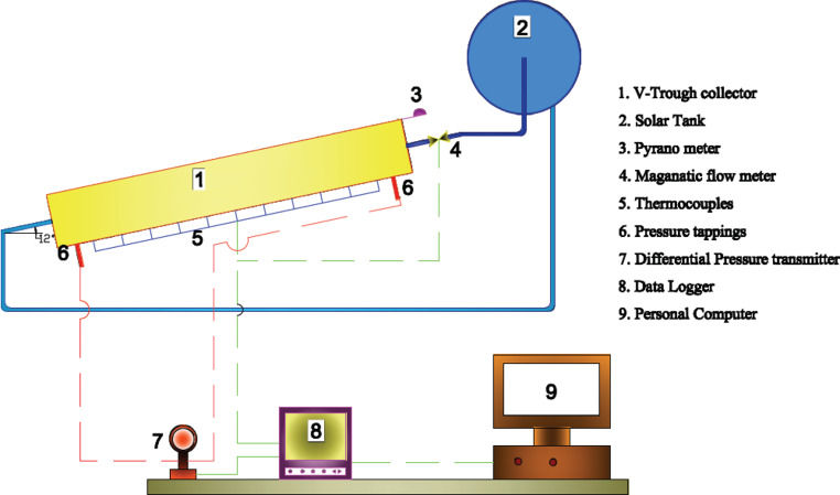
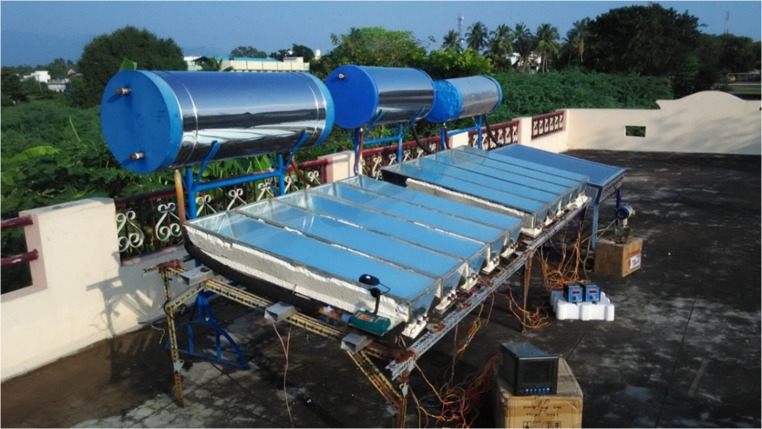
Two 1.1 cm diameter and 100 cm long riser tubes are covered by a 200 mm wide black coated absorber plate and two reflectors at a 120° angle to the absorber plate, making a V-trough unit (V.T.). In the same way, five numbers of V.T. are connected in a series. A typical lower header joins all the riser tubes on the bottom side, and an upper header does the same for all the top ones. The top side of the absorber plate is covered with 3 mm thick high transmittance glazing glass, and both ends of the V.T. reflector are covered with Trapezium-shaped floating glass. Finally, as shown in Fig. 1, the unit is tilted to the south at a 12⁰ angle. Figure 2 displays a pictorial view of the V.T.

Figure 1.

Schematic diagram of an experimental setup.

Figure 2.

Pictographic view of the experimentation setup.

Cold water is drawn into the collector from the storage tank through the bottom header and is distributed uniformly throughout the riser tubes. The absorber plate’s convectional transfer of heat heats of this fluid. Hot water is collected and stored in a storage tank in the top header. The stored water’s driving power is raised until the input and output temperatures are equal.

Twist with a V cut and a square cut: technical details

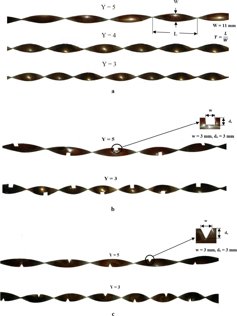
Experiments were carried out using strips of copper, each measuring 100 centimeters long (l), 1.1 centimeter in width (w) and 0.3 millimeters in thickness. Y = 3 to 5 is the twist ratio of the helix after it has been rotated 180 degrees. Twisted tape is cut in half from top to bottom at the alternative node on the outer surface, resulting in a 3 mm wide (w) by 3 mm deep square cut (d_e). Figure 3 shows a V-cut and square-cut with 3 mm wide and 3 mm deep dimensions.

Figure 3.

a. Geometry of Helix twisted tape - Conventional. b. Geometry of Helix twisted tape - Square cut. c. Geometry of Helix twisted tape - V - cut.

Instrumentation

With a precision of 0.1 °C, the RTD monitors the water intake and output temperature, checks every minute and is recorded in the Datalogger. The T-type thermocouple was welded using a thermocouple wire welding equipment with an accuracy of 0.5 °C at six spots along the 100 cm-long absorber plate and a 25 cm gap in each riser tube. The pressure reduction is measured using the Honeywell pressure transmitter, which has a 0.1% accuracy. Solar insolation is measured using a Kipp & Zonen Pyranometer. The water mass flow rate is monitored using ultra-low flow meters with a 1.0% accuracy rate.

Procedure for the experiment

This experiment is being conducted at Aditya University, which is located in Surampalam, India (17.0895° North, 82.0668° East). Between the months of March and May of 2023, the data might be collected. All of the research was conducted on a daily basis between the hours of 9:30 a.m. and 4:30 p.m. At the beginning of each day, fresh water is added to the water supply. A data logger is used to record the water temperatures at the entry and exit of each riser tube, as well as the temperature of the absorber plate, and then the average number of these temperatures is calculated. The mass flow rate of water, the differential pressure of the tube’s intake and exit, solar intensity, the air temperature, the absorber plate temperature, and the water temperatures at the inlet and outlet were all recorded at regular intervals of fifteen minutes. On days that were bright and sunny, the experiment was carried out with a relative humidity of around 71%, a maximum air temperature of 40 °C, and a maximum wind speed of 3.7 m per second. Beginning in the morning and continuing until 1:00 p.m., the intensity of the sun gradually climbed until it reached its highest point at 1:00 p.m., and then gradually declined until 4:00 p.m.

Data reduction equation

The Nu, FF, and η of a VTSWH with helix-twisted tape inserts (plain, square cut, and V-cut) and without helix-twisted tape inserts were calculated using the experimental data.

Heat transfer

The equation below can be used to determine the heat transfer (Q) rate in a single riser tube⁵.

1

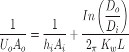
The mass flow rate, C_pand the temperature differential between the fluid outflow and input are linked to the heat transfer rate (Q)⁵. Thus

2

Combining Eqs. 1 and 2 yields the value of internal convection. The experimental Nu value is calculated using the equation The bulk mean temperature T_m is used to compute all fluid thermophysical characteristics.

Friction factor (FF)

Because of the frictional resistance that exists between the fluid and the tube wall, the pressure of the fluid decreases as it passes through the tube at a certain velocity. Every single tube is equipped with a differential pressure transducer, which is responsible for monitoring and calculating the average pressure decrease.

The FF is determined using the following formula⁵:

3

where △P is the pressure drop over the length (L).

Thermal performance (η)

The Hottel – Whillier – Bliss equation is used to determine the solar water heater’s thermal performance⁵:

4

The following equations were used to compute the heat removal factor (F._R.), heat loss coefficient (Ul), and transmittance-absorbance (τα)⁵

5

Experimental result

The helical twist induced swirl flow enhances heat transfer as compared to a plain tube. In addition to increasing the impact of particle mixing, the V-cut in the helix twisted tape produced a secondary flow in the fluid motion. The temperature gradient is increased by this occurrence, which is linked to the mixing of fluid flow with the tube’s surface area and core. Thus, with V-cut helix twist tape, a larger Nusselt number is achieved. When comparing square cut helix twisted tapes to V-cut helix twisted tapes, the square cut helix twisted tape has the highest amount of material removed, which lowers the secondary fluid flow velocity.

Data and its pre-processing

This work utilised four machine learning models to predict three outputs or dependent variables: Nu, f, and η. Eight independent variables were used as inputs to the ML models to predict the outcomes. Solar intensity (H_t), inlet water temperature (T_i), outlet water temperature (T_o), riser tube temperature (T_p), absorber plate temperature (T_w), ambient temperature (T_a), Velocity of water (V_w) and the twist ratio of inserts(Y) were employed as independent variables. For this investigation, a total of 162 unique entries were used. Table 1 below describes the dataset utilised for modelling. These results came from tests employing the twisted tape setup described in the Experimental Setup section.

Table 1.

Dataset description.

Attribute	Sample No	Mean Value	Standard deviation	Min Value	25%	50%	75%	Max Value
I (t)	162	930.056	154.033	602	805	948.5	1076	1144
Ti	162	55.86	11.90	35.50	45.30	57.08	66.18	74.60
To	162	59.37	11.94	37.50	49.15	61.28	69.89	76.70
Tp	162	59.77	11.97	37.70	49.45	61.78	70.28	76.90
Tw	162	66.42	8.77	49.40	59.04	66.35	73.90	82.60
Ta	162	33.80	1.72	30.20	32.50	34.10	35.20	36.40
Vw	162	0.0842	0.0111	0.0605	0.0750	0.0841	0.0932	0.1113
Y	162	4	1.0031	3	3	4	5	5
Nu	162	14.15	2.13	9.30	12.65	14.05	15.71	19.44
F	162	0.1074	0.0048	0.0975	0.1039	0.1073	0.1107	0.1179
Η	162	66.07	11.81	36.28	58.21	68.70	75.57	84.25

Additionally, before modelling, with the help of Matlab programming, correlations between the independent factors and the dependent variables were observed. The determined associations are included in Table 2. It can be shown that the solar intensity and ambient temperature parameters have a significant and positive connection with the dependent variable, which is the Nu. The Pearson correlation values for these two parameters are 0.7364971 and 0.73, both of which are positive. On the other hand, the output variable, also known as FF, exhibits a negative correlation with the same two independent variables. The Pearson correlation values of -0.860686 and − 0.88 were found to be relatively comparable. There is a negative correlation between each of the other parameters being considered. There is a significant and positive link between the Solar intensity and the temperature outside, as indicated by the Pearson coefficients of 0.901180059 and 0.93 for η. In addition to this, there is a minor negative association with all of the other components.

Table 2.

The independent and dependent variables’ determined correlations.

Input /Output	Nu	FF	η
Solar intensity (I(t))	0.736497155	-0.860686749	0.901180059
Inlet temperature	-0.121700852	-0.129893917	0.137680071
Outlet temperature	-0.078402787	-0.180628388	0.195011949
Tube temperature	-0.078142782	-0.19016665	0.199890021
Absorber plate temperature	-0.504621	-0.183191258	0.033714789
Atmosphere temperature	0.73	-0.88	0.93
Twist ratio	-0.57	-0.42	-0.28

‘X’ and ‘y’ are two distinct data frames that each include the independent and dependent variables. The variables were divided into training and testing groups, with 80% of the data utilised for training and 20% set aside for model testing.

Prediction models

In the present work, four models (ANFIS, G.L.R., RT and SVM model) have been used to predict the thermal performance of the VTSWH. The performance of all these models has also been compared with the Nu, f, and η of the experimental data.

Adaptive neuro-fuzzy inference system (ANFIS)

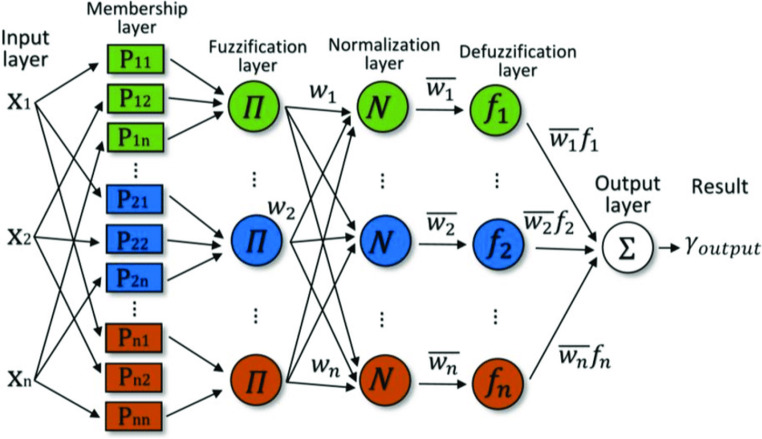
It is a Neuro-Fuzzy system (N.F.S.) often used to solve regression issues. ANFIS starts with constructing a Fuzzy Inference System (F.I.S.) and tuning its Membership Function (M.F.) parameters using Neural Networks. This adjustment helps the F.I.S. in learning from the data it is modelling. The N.F.S. is built using a fuzzy approach enhanced with neural networks, which aids the model in improving features such as adaptability and flexibility. This paper examines the Takagi-Sugeno Neuro-Fuzzy Inference System, a typical ANFIS model. The membership functions in ANFIS are learned using the backpropagation technique, whereas the coefficients for the system’s rules are obtained using the least mean square method. Figure 4 depicts the ANFIS schema. The inputs of ANFIS are converted to output via a series of six layers. The ANFIS is created using the MATLAB functions genfis2() and anfis( ).

Figure 4.

Structure of the ANFIS model.

Generalised Linear Regression (GLR)

It is more flexible when the response variables have arbitrary distributions other than the normal distribution. G.L.R.s are generalised linear regression models in which a link function links the response variable and predictors. The size of the variance of each measurement may be modelled as a function of the predictors in G.L.R.s. The target values are expected to be linearly connected to the input variables in G.L.R. However, finding a straight line (or hyperplane) that passes through all of the points of the input variables is very hard.

On the other hand, the linear regression model is created by minimising the difference between the observed and predicted values. The fitglm( ) function in MATLAB is used for the experimentation. The model assumes the following form³⁷:

6

7

Where

is the regression coefficient vector

y_j

j^th observed response

is the j^th input variables vector

j^th predicted response

e

error term

Regression tree

A regression tree is a decision tree that predicts continuous-valued outputs rather than discrete outputs for regression. To comprehend a Regression Tree, one must first comprehend the concept of decision trees. A decision tree is a kind of tree that may be used to help make a choice. The decision tree helps predict an output based on the relevant input variables. A decision tree is utilised in data analysis and for different predictions. A classification tree and a regression tree are two forms of decision trees. The Classification Tree is a decision tree with a categorical target variable, while the Regression Tree has a continuous target variable, as shown in Fig. 5. The fitrtree( ) tool in MATLAB is used to generate the Regression Tree for this study.

Figure 5.

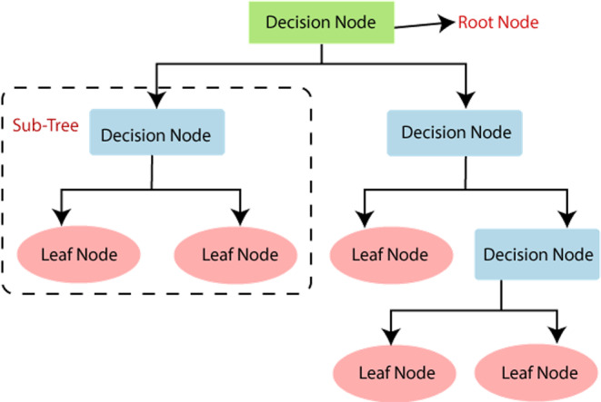
Structure of regression tree model.

Support vector machines (SVM)

In accordance with the statistical learning theory, the concept of “kernel” is commonly utilized for learning tasks. Kernel machines offer a flexible structure that may be customized for different applications and domains using several kernel functions, such as linear, radial basis, polynomial, or sigmoid, as seen in Fig. 6. The concepts of SVM enable it to successfully address prediction and classification difficulties. The S.V.R. model is created using subsets of training data, specifically focusing on data that is in close proximity to the model’s prediction cost function. The fitrsvm() function in MATLAB is utilized for experimenting.

Figure 6.

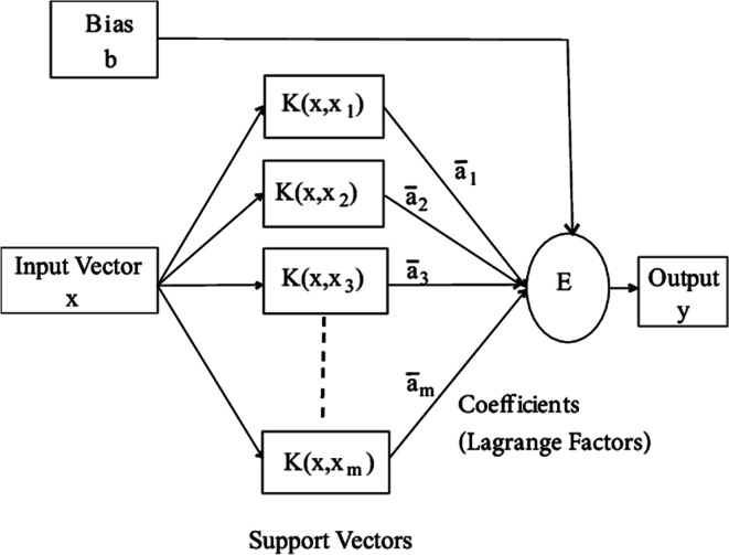
Structure of regression tree model.

Results and discussion

The performance of the models was evaluated using conventional coefficients of determination such as M.A.E., RMSE, and R²values, which were validated using test data³⁸. Tables 3, 4 and 5 show the values that were addressed for Nu, f and η. Compared to the performances of the G.L.R., R.T., and SVM models, the ANFIS model has the lowest error and the highest R² value. The ANFIS model’s MMRE, RMSE, and R² values were 0.3429, 0.0805, and 0.9990 for Nu, 0.2368, 0.0004 and 0.9942 for f, and 0.3242, 0.4534, and 0.9985 for η, respectively.

Table 3.

Coefficients of determination for Nu models developed with test data.

Coefficient of Determination	ANFIS	GLR	RT	SVM
R2	0.9990	0.9961	0.9562	0.9280
RMSE	0.0805	0.1259	0.5107	0.5461
MMRE	0.3429	0.6919	2.9022	3.1711

Table 4.

Coefficients of determination for FF models developed with test data.

Coefficient of determination	ANFIS	GLR	RT	SVM
R2	0.9966	0.9683	0.9810	0.9560
RMSE	0.0004	0.0009	0.0008	0.0015
MMRE	0.2368	0.6742	0.5712	1.0985

Table 5.

Coefficients of determination for η models developed with test data.

Coefficient of determination	ANFIS	GLR	RT	SVM
R2	0.9997	0.9976	0.9845	0.9614
RMSE	0.4534	0.6762	1.8399	2.2590
MMRE	0.3242	0.7679	2.1990	2.8437

Due to its lowest error and highest R² value, which is extremely near to unity and demonstrates the model’s correctness, the ANFIS model is superior to the G.L.R., R.T., and SVM models in light of the above information. After ANFIS, the G.L.R. model outperforms R.T. and SVM.

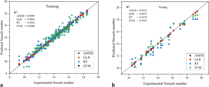
Figure 7a and b illustrate the predicted and experimental nusselt values for each iteration of the training and testing sets. It is evident that compared to the other three models, the projected outcomes of ANFIS are more closely matched with the regression line. The performance was good for ANFIS, with an R² score of 0.999 and 0.9976 for training and testing data iteration, respectively. But for training data iteration, G.L.R., R.T. and SVM models give the R² value of 0.9961, 0.9562 and 0.928, and for testing data iteration G.L.R., R.T. and SVM models give the R² value of 0.9975, 0.9155 and 0.951 respectively.

Figure 7.

a. Comparison of ANFIS, G.L.R., R.T., and SVM model predicted Nu with experimental results for training. b. Comparison of experimental with ANFIS, G.L.R., R.T. and SVM predicted Nu for testing.

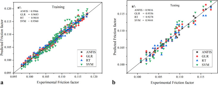
Figure 8a and b illustrate the predicted and experimental FFs for every iteration of the training and testing sets. The ANFIS model’s anticipated outcomes exhibit a higher degree of alignment with the regression line compared to the other three models. ANFIS had strong performance, as evidenced by an R² value of 0.9966 for the training data iteration and 0.9816 for the testing data iteration. The G.L.R., R.T., and SVM models provide R² values of 0.9683, 0.981, and 0.956, respectively, when applied to the training data. For the testing data, the corresponding R² values are 0.9556, 0.9278, and 0.944. The aforementioned result indicated that ANFIS had accurately predicted the FF.

Figure 8.

a. Comparison of ANFIS, G.L.R., R.T., and SVM model predicted FF with experimental results for training. b. Comparison of experimental with ANFIS, G.L.R., R.T. and SVM predicted FF for testing.

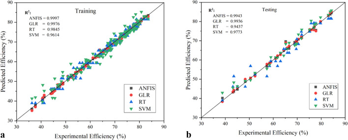
Figure 9a and b demonstrate the predicted and experimental η for each iteration of the training and testing sets. Compared to the predictions of the other three models, those of ANFIS are more closely matched to the regression line. ANFIS worked well, with an R² value of 0.9997 for the training data iteration and 0.9943 for the testing data iteration. But for iterating on training data, G.L.R., R.T., and SVM models offer R² values of 0.9976, 0.9845, and 0.9614, respectively, and 0.9936, 0.9437, and 0.9773 for iterating on testing data.

Figure 9.

a. Comparison of ANFIS, G.L.R., R.T., and SVM model predicted η with experimental results for training. b. Comparison of experimental with ANFIS, G.L.R., R.T. and SVM predicted η for testing.

The above outcome demonstrated that ANFIS had more precisely forecast. In this situation, ANFIS has predicted the Nu and η more accurately than the f since the f outcomes are more distributed than the Nu and η.

The residual errors obtained while predicting the Nu by all the training models are presented in Fig. 10. In that, it can be observed that the least deviation of the residuals obtained from the zero-axis line is for ANFIS, followed by G.L.R., while the most deviation was while predicting with SVM followed by R.T. This sums up the poor performance of the latter two models while predicting the Nu from training data. The maximum relative error ANFIS, G.L.R., R.T. and SVM models were ± 1.99%, ± 3.53%, ± 11% and ± 16.42%, respectively. It is evident that among ANFIS, G.L.R., R.T. and SVM models, the average maximum relative error of the ANFIS model has the lowest value. Compared to G.L.R., R.T., and SVM models, the ANFIS model predicts the outcomes more precisely.

Figure 10.

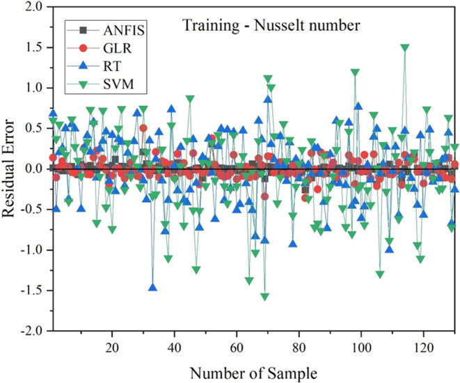
Residual error of ANFIS, G.L.R., R.T., SVM model w.r.t Nu for training.

A similar trend can also be observed in Fig. 11, representing the residuals obtained while predicting the FF for training data. The maximum relative error ANFIS, G.L.R., R.T. and SVM models were found to be ± 0.991%, ± 2.014%, ± 1.584% and ± 2.51%, respectively. While predicting FF, though ANFIS still performed the best, its performance cannot be compared to predicting the other two output variables.

Figure 11.

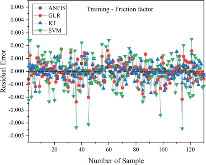
Residual error of ANFIS, G.L.R., R.T., SVM model w.r.t FF for training.

Figure 12 illustrates the residuals found while estimating the η using training data. It was found that the maximum relative error for the ANFIS, G.L.R., R.T., and SVM models, respectively, was ± 1.88%, ± 4.05%, ± 6.9%, and ± 15.53%. While ANFIS outperformed all other models in forecasting η, its performance cannot be compared to the other two output variables.

Figure 12.

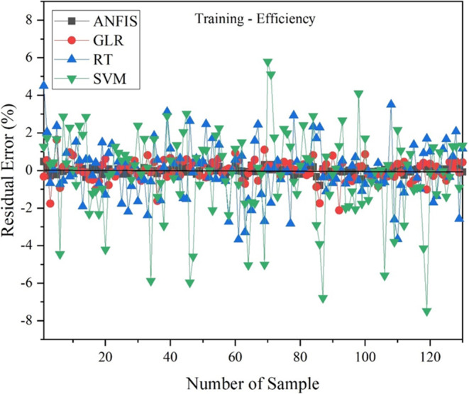
Residual error of ANFIS, G.L.R., R.T., SVM model w.r.t η for training.

The residuals obtained are unmatchable to that of the training data. However, suppose only the testing data is considered. In that case, the residuals obtained by ANFIS for Nu and η are the best among all the models, almost similar. They have not deviated much from the zero-axis line. The G.L.R. model is next best to ANFIS, followed by R.T., while SVM is the worst-performing model. In predicting FF, almost all the models have generated substantial residuals compared to Nu and η. In this case, also, ANFIS is the best-performing model.

By giving testing data as inputs to the models for prediction, graphs were also produced along comparable axes. Figures 13, 14, and 15 show the experimental and predicted outcomes for the Nu, FF and η, for testing. ANFIS performs better than G.L.R., SVM and R.T. models with a minimum error of about ± 2.86%, ± 1.42%, and ± 6.32% for Nu, FF and η, respectively. It is not the case for SVM and R.T., for which the values typically coincide with the trend line, indicating its poor performance, with SVM being the worst-performing model.

Figure 13.

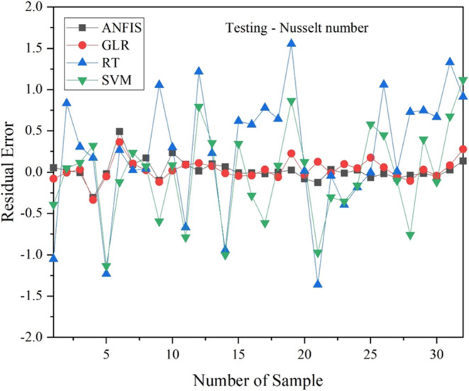
Residual error of ANFIS, G.L.R., R.T., SVM model w.r.t Nu for testing.

Figure 14.

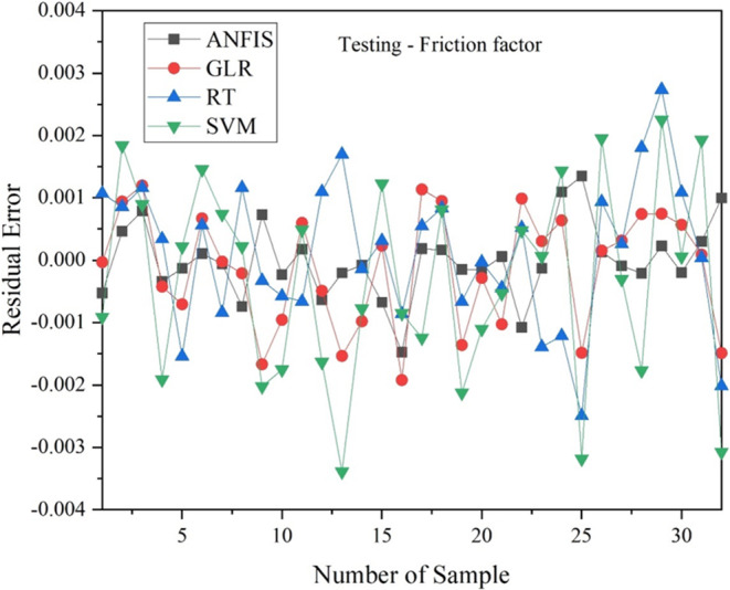
Residual error of ANFIS, G.L.R., R.T., SVM model w.r.t FF for testing.

Figure 15.

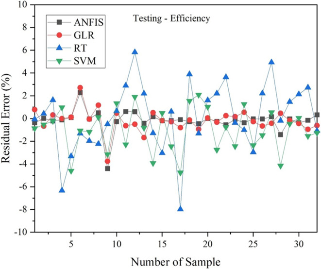
Residual error of ANFIS, G.L.R., R.T., SVM model w.r.t η for testing.

The results mentioned above demonstrate that all four models considered in the current study can accurately predict Nu, FF, and η; however, the ANFIS model is the most suited since it makes predictions with less error than the other models. So, with a confidence level above 95%, the ANFIS model accurately predicts the data.

Conclusion

In the current study, square-cut twisted tape (SCTT) and V-cut twisted tape (VCTT) with two different twist ratios, 3 and 5, have been utilized to forecast the thermal performance of a V-trough solar water heater (VTSWH) using four different types of neural models (ANFIS, G.L.R., R.T., and SVM). The temperature outside, the mass flow rate of water, the temperature inside and outside the water, the temperature of the absorber plate, the temperature within the tube, solar intensity, and the twist ratio are the independent variables. Nu, FF, and η are the output, or dependent, variables. The identical set of parameters are applied to all four models. There were 162 data sets utilized in all. R², RMSE, and MMRE have been used to compute and compare the performance of all four models. The following conclusions have been listed below:

• Using the ANFIS, G.L.R., R.T., and SVM techniques, the correlation coefficient (R²) values for the Nu were found as 0.9990, 0.9961, 0.9562, and 0.9280, for the FF 0.9966, 0.9683, 0.9810 and 0.9560, and η 0.9997, 0.9976, 0.9845, and 0.9614, respectively.

• Based on the result, ANFIS model is the most effective of the four strategies studied.

• The ANFIS model outperformed the other models regarding Nu, FF, and η, with RMSE values of 0.0805, 0.0.000363, and 0.4533.

• According to the above data, the VTSWH thermal performance predicted using the ANFIS approach has the highest accuracy.

• The proposed model will be most helpful for estimating the performance of the new solar water heating system since it does not require a detailed investigation of heat transfer analysis.

Abbreviations

ANN

Artificial Neural Network

ANFIS

Adaptive Neuro-Fuzzy Inference System

G.L.R

Generalised linear regression

R.T

Regression tree

SVM

Support Vector Machine

MAE

Mean Absolute Error

ML

Machine Learning

NN

Neural Network

R²

Coefficient of Determination

RMSE

Root Mean Square Error

MMRE

Mean Magnitude of Relative Error

SWH

Solar Water Heater

TSS

Tubular Solar Still

Nu

Nusselt Number

FF

Friction Factor

Symbols

H_t

Solar intensity, W/m²

Δp

Pressure drop, N/m²

V_a

Velocity of flow, m/s

T_a

Ambient temperature,⁰C

T_p

Riser tube temperature,⁰C

T_i

Inlet water temperature, ⁰C

T_o

Outlet water temperature, ⁰C

V_w

Velocity of water , m/s

K_w

Thermal Conductivity of water (W/mK)

m

Mass flow rate (kg/s)

η

Thermal efficiency, %

Author contributions

A.S, S.R.S & M.S.R: Conceptualization, A.S, E.P.V, A.K.C, K.K & N.H Methodology & Formal analysis, A.S Writing – original draft.

Data availability

The datasets generated during and/or analysed during the current study are available from the corresponding author on reasonable request.

Declarations

Competing interests

The authors declare no competing interests.

References

- 1.Kumar, A. & Prasad, B. N. Investigation of twisted tape inserted solar water heaters - heat transfer, friction factor and thermal performance results. Renew. Energy.19, 379–398 (2000). [Google Scholar]
- 2.Saravanan, A., Senthilkumaar, J. S. & Jaisankar, S. Experimental studies on heat transfer and friction factor characteristics of twist inserted V-trough thermosyphon solar water heating system. Energy. 10.1016/j.energy.2016.06.103 (2016). [Google Scholar]
- 3.Saravanan, A., Senthilkumaar, J. S., Jaisankar, S. & Ananth, J. Influence of helix twisted tape on heat transfer and friction factor in forced circulation V-trough solar water heater. Int. J. Sustain. Energy. 163–176. 10.1080/14786451.2018.1476352 (2019).
- 4.Saravanan, A., Senthilkumaar, J. S. & Jaisankar, S. Experimental studies on heat transfer and friction factor characteristics of twist inserted V-trough thermosyphon solar water heating system. Energy. 112, 642–654 (2016). [Google Scholar]
- 5.Saravanan, A., Senthilkumaar, J. S. & Jaisankar, S. Performance assessment in V-trough solar water heater fitted with square and V-cut twisted tape inserts. Appl. Therm. Eng.10.1016/j.applthermaleng.2016.03.088 (2016). [Google Scholar]
- 6.Murugan, M., Vijayan, R., Saravanan, A. & Jaisankar, S. Influence of corrugated booster reflectors in a centrally finned twist inserted solar thermal collector on heat transfer and thermal performance characteristics. J. Heat. Transf.141, 062001 (2019). [Google Scholar]
- 7.Murugan, M., Vijayan, R., Saravanan, A. & Jaisankar, S. Performance enhancement of centrally finned twist inserted solar collector using corrugated booster reflectors. Energy.168, 858–869 (2019). [Google Scholar]
- 8.Murugan, M., Vijayan, R. & Saravanan, A. Improving performance of a trapezoidal-trough thermosyphon solar collector using peripherally wing-cut swirl generator. Int. J. Green. Energy.16, 1196–1209 (2019). [Google Scholar]
- 9.Nikkonen, S., Afara, I. O., Leppänen, T. & Töyräs, J. Artificial neural network analysis of the oxygen saturation signal enables accurate diagnostics of sleep apnea. Sci. Rep.9, 1–9 (2019). [DOI] [PMC free article] [PubMed] [Google Scholar]
- 10.Chauhan, R., Dumka, P. & Mishra, D. R. Modelling conventional and solar earth still by using the LM algorithm-based artificial neural network. Int. J. Ambient Energy. 1–1310.1080/01430750.2019.1707113 (2020).
- 11.Rishika Chauhan, S., Sharma, R., Pachauri, P. & Dumka, D. R. M. Experimental and theoretical evaluation of thermophysical properties for moist air within solar still by using different algorithms of artificial neural network. J. Energy Storage.30, 101408 (2020). [Google Scholar]
- 12.Mohammed Shadi, S., Abujazar, F., Suja, I. A., Ibrahim, A. E. & Kabeel, S. S. Productivity modelling of a developed inclined stepped solar still system based on actual performance and using a cascaded forward neural network model. J. Clean. Prod.170, 147–159 (2018). [Google Scholar]
- 13.Mashaly, A. F., Alazba, A. A., Al-Awaadh, A. M. & Mattar, M. A. Predictive model for assessing and optimizing solar still performance using artificial neural network under hyper arid environment. Sol Energy.118, 41–58 (2015). [Google Scholar]
- 14.Mashaly, A. F. & Alazba, A. A. Thermal performance analysis of an inclined passive solar still using agricultural drainage water and artificial neural network in arid climate. Sol Energy.153, 383–395 (2017). [Google Scholar]
- 15.Mashaly, A. F. & Alazba, A. A. Comparison of ANN, MVR, and SWR models for computing thermal efficiency of a solar still. Int. J. Green. Energy.13, 1016–1025 (2016). [Google Scholar]
- 16.Sohani, A., Hoseinzadeh, S., Samiezadeh, S. & Verhaert, I. Machine learning prediction approach for dynamic performance modeling of an enhanced solar still desalination system. J. Therm. Anal. Calorim.147, 3919–3930 (2022). [Google Scholar]
- 17.Mashaly, A. F. & Alazba, A. A. Neural network approach for predicting solar still production using agricultural drainage as a feedwater source. Desalin. Water Treat.57, 28646–28660 (2016). [Google Scholar]
- 18.Bagheri, A., Esfandiari, N., Honarvar, B. & Azdarpour, A. First principles versus artificial neural network modelling of a solar desalination system with experimental validation. Math. Comput. Model. Dyn. Syst.25, 453–480 (2020). [Google Scholar]
- 19.Erenturk, S. & Erenturk, K. Comparisons of novel modeling techniques to analyze thermal performance of unglazed transpired solar collectors. Meas. J. Int. Meas. Confed. 116, 412–421 (2018). [Google Scholar]
- 20.Ghritlahre, H. K. P. Exergetic performance prediction of solar air heater using MLP, GRNN and RBF models of artificial neural network technique. J. Environ. Manage.223, 566–575 (2018). [DOI] [PubMed] [Google Scholar]
- 21.Harish Kumar Ghritlahre & Radha Krishna Prasad. Prediction of heat transfer of two different types of roughened solar air heater using Artificial neural network technique. Therm. Sci. Eng. Prog. 8, 145–153 (2018). [Google Scholar]
- 22.Hikmet Esen, F., Ozgen, Esen, M. & Sengur, A. Artificial neural network and wavelet neural network approaches for modelling of a solar air heater. Expert Syst. Appl.36, 11240–11248 (2009). [Google Scholar]
- 23.Ghritlahre, H. K. Purvi Chandrakar & Ashfaque Ahmad. Application of ANN model to predict the performance of solar air heater using relevant input parameters. Sustain. Energy Technol. Assessments.40, 100764 (2020). [Google Scholar]
- 24.Shreyas, P., Shetty, Nayak, S., Kumar, S. & Karanth, K. V. Thermo-hydraulic performance prediction of a solar air heater with circular perforated absorber plate using Artificial neural network. Therm. Sci. Eng. Prog. 23, 100886 (2021). [Google Scholar]
- 25.Rahmati Aidinlou, H. & Nikbakht, A. Fuzzy-based modeling of thermohydraulic aspect of solar air heater roughened with inclined broken roughness. Neural Comput. Appl.34, 2393–2412 (2022). [Google Scholar]
- 26.Rahmati, A. & Nikbakht, A. M. Intelligent modeling of thermohydraulic behavior in solar air heaters with artificial neural networks. Neural Comput. Appl.31, 3279–3293 (2019). [Google Scholar]
- 27.Ghritlahre, H. K. & Prasad, R. K. Development of optimal ANN Model to estimate the thermal performance of roughened solar air heater using two different learning algorithms. Ann. Data Sci.5, 453–467 (2018).
- 28.Caner, M., Gedik, E. & Keçebas, A. Investigation on thermal performance calculation of two type solar air collectors using artificial neural network. Expert Syst. Appl.38, 1668–1674 (2011).
- 29.Chaibi, Y., Malvoni, M., Rhafiki, E., Kousksou, T., Zeraouli, Y. & T. & Artificial neural-network based model to forecast the electrical and thermal efficiencies of PVT air collector systems. Clean. Eng. Technol.4, 100132 (2021). [Google Scholar]
- 30.Kalogirou, S. A., Panteliou, S. & Dentsoras, A. Artificial neural networks used for the performance prediction of a thermosiphon solar water heater. Renew. Energy.. 18, 87–99 (1999). [Google Scholar]
- 31.Sadeghi, G., Nazari, S., Ameri, M. & Shama, F. Energy and exergy evaluation of the evacuated tube solar collector using Cu2O/water nanofluid utilizing ANN methods. Sustain. Energy Technol. Assess. 37, 100578 (2020).
- 32.Souliotis, M., Kalogirou, S. & Tripanagnostopoulos, Y. Modelling of an ICS solar water heater using artificial neural networks and TRNSYS. Renew. Energy.34, 1333–1339 (2009). [Google Scholar]
- 33.Tomy, A. M., Ahammed, N., Subathra, M. S. P. & Asirvatham, L. G. Analysing the performance of a flat plate solar collector with silver/water nanofluid using artificial neural network. Procedia Comput. Sci.93, 33–40 (2016).
- 34.Kulkarni, M. V., Deshmukh, D. S. & Shekhawat, S. P. An innovative design approach of hot water storage tank for solar water heating system using artificial neural network. Mater. Today Proc.46, 5400–5405 (2020).
- 35.Wongsuwan, W. & Kumar, S. Forced circulation solar water heater performance prediction by TRNSYS and ANN. Int. J. Sustain. Energy. 24, 69–86 (2005). [Google Scholar]
- 36.Saravanan, A., Satyajeet Parida, M., Murugan, M. S., Reddy, P. & Bora, S. R. S. Performance estimation of tubular solar still with a wicked rotating drum using DT, LR, and KNN techniques of machine learning. Neural Comput. Appl.36, 1–11 (2022). [Google Scholar]
- 37.Tsimikas, J. V., Bantis, L. E. & Georgiou, S. D. Inference in generalized linear regression models with a censored covariate. Comput. Stat. Data Anal.56, 1854–1868 (2012). [Google Scholar]
- 38.Tripathy, D. P., Parida, S. & Khandu, L. Safety Risk Assessment and Risk Prediction in Underground Coal Mines using machine learning techniques. J. Inst. Eng. Ser. D. 8, 6–15 (2021). [Google Scholar]
Associated Data
This section collects any data citations, data availability statements, or supplementary materials included in this article.
Data Availability Statement