Water quality–fisheries tradeoffs in a changing climate underscore the need for adaptive ecosystem–based management

Significance

Our study showcases an approach to assess nutrient management decision-making in aquatic ecosystems. By combining fisheries data with reconstructed nutrient loads and hypoxic extent during the past century, we demonstrate why nutrient abatement plans designed to curtail Lake Erie hypoxia appear too restrictive in today’s climate yet may be insufficient in the future. Beyond illustrating how nutrient management can cause water quality–fisheries tradeoffs that can vary with climate change, we offer a rare example of nutrient-driven hypoxia shaping long-term fisheries harvest dynamics in a large ecosystem. Ultimately, our study highlights why adaptive ecosystem–based management that uses simple predictive models to assess tradeoffs between management priorities over long timescales can help sustain valued services in ecosystems experiencing change.

Abstract

Changes driven by both unanticipated human activities and management actions are creating wicked management landscapes in freshwater and marine ecosystems that require new approaches to support decision-making. By linking a predictive model of nutrient- and temperature-driven bottom hypoxia with observed commercial fishery harvest data from Lake Erie (United States–Canada) over the past century (1928–2022) and climate projections (2030–2099), we show how simple, yet robust models and routine monitoring data can be used to identify tradeoffs associated with nutrient management and guide decision-making in even the largest of aquatic ecosystems now and in the future. Our approach enabled us to assess planned nutrient load reduction targets designed to mitigate nutrient-driven hypoxia and show why they appear overly restrictive based on current fishery needs, indicating tradeoffs between water quality and fisheries management goals. At the same time, our temperature results show that projected climate change impacts on hypoxic extent will require more stringent nutrient regulations in the future. Beyond providing a rare example of bottom hypoxia driving changes in fishery harvests at an ecosystem scale, our study illustrates the need for adaptive ecosystem–based management, which can be informed by simple predictive models that can be readily applied over long time periods, account for tradeoffs across multiple management sectors (e.g., water quality, fisheries), and address ecosystem nonstationarity (e.g., climate change impacts on management targets). Such approaches will be critical for maintaining valued ecosystem services in the many aquatic systems worldwide that are vulnerable to multiple drivers of environmental change.

Human-caused environmental change is a global problem threatening our ability to sustain valued ecosystem services. Humans have altered aquatic and terrestrial ecosystems in both conspicuous (1, 2) and surprising (3) ways, with altering nutrient availability being among the most pervasive, especially in coastal ecosystems with vast agriculture watersheds or large human populations (4, 5). A rich literature exists on the causes and consequences of excessive nutrient inputs that often come from unplanned loads [e.g., cultural eutrophication; (6–8)], as well as through nutrient abatement [i.e., planned oligotrophication; (9–11)]. Yet, considerable uncertainty remains concerning the difficult management landscape that can be created by altering nutrient inputs, which can differentially impact valued ecosystem components (sense ref. 12).

Most conspicuous in both freshwater and marine aquatic ecosystems are tradeoffs between water quality and fisheries. Theoretically, every fish population has an optimal level of nutrients, high enough to support prey production, but not so high as to degrade habitat [via hypoxia, reduced water clarity, and harmful algal blooms (HABs)] such that growth, survival, and reproductive fitness are reduced (13). This nonlinear response to nutrient availability, combined with population-specific tolerances to water quality impairments (10, 14), can create a management dilemma because reducing nutrient inputs to achieve water quality goals can simultaneously promote and harm fish production depending on species tolerances (12). Thus, a need exists to consider possible tradeoffs between ecosystem components when setting management targets. Lacking in most ecosystems, however, are the needed data and tools to understand and assess these tradeoffs both now in the face of future human-driven environmental change.

As suggested by Sinclair et al. (12), tradeoffs between water quality and fisheries can best be identified and assessed through ecosystem–based management (EBM), which facilitates discussion among stakeholders, supports interdisciplinary research and monitoring, and employs cooperative decision-making (15–17). If done well, EBM will address interactions across spatiotemporal scales, within and among socioecological systems, and among stakeholders and rightsholders interested in the present and future health of the ecosystem (18–20). EBM should also be done iteratively through adaptive management: defining the problem, identifying goals and evaluation criteria, predicting outcomes, evaluating tradeoffs, making decisions, implementing actions, monitoring and evaluating outcomes, and then adjusting objectives or approaches as necessary (19, 21). Unfortunately, most of the world’s ecosystem services are not currently being managed in an adaptive EBM context (22–24), which is hampering our ability to keep our ecosystems and services that they provide resilient.

This lack of EBM implementation has many causes, with inadequate science support being one of them (20, 24, 25). A key gap that has limited effective EBM in many places is the lack of models that can identify and assess multisectoral (e.g., water quality vs. fishery) tradeoffs yet are simple enough for nonscientists to leverage. Given that predictive models often fail the test of time (26, 27), such models should also be easily reassessed and updated. This is particularly true in the face of climate change, which is likely to alter relationships between human (e.g., nutrient) inputs and water-resource outcomes (28–30).

The need for adaptive EBM is especially critical in large aquatic ecosystems, including the world’s Great Lakes (e.g., North American; East African Rift Valley) and coastal marine ecosystems, which are facing multiple anthropogenic stressors (31–34). As with large marine ecosystems (13, 35), strong relationships between ecosystem productivity and fisheries production have been documented in lakes (36, 37), with proxies of both often showing species-specific unimodal responses such that some fisheries will “win” while others will “lose” as water quality changes (10, 12, 13). Such tradeoffs between water quality and fisheries production have been explained by changes in habitat quantity (e.g., prey availability) and habitat quality (e.g., bottom hypoxia). While documented bottom–up effects of increased nutrients have validated the ascending portion of this unimodal curve (e.g., ref. 38), long-term consequences of bottom hypoxia on fisheries yields of large-bodied species at population or ecosystem scales have remained largely elusive in most ecosystems (39–41).

This difficulty in characterizing long-term effects of nutrient-driven hypoxia on fisheries is partly due to its multifaceted effects on ecosystems (40–43); however, a lack of long-term historical bottom dissolved oxygen (DO) data can also be a key limiter. Thus, methods to quantify historical variation in DO and its influence on fisheries production remain vital in many ecosystems, including Lake Erie (United States–Canada), which has experienced large swings in hypoxia and fisheries during the past half-century due to both altered nutrient loading and climate variation (29, 44–46). To illustrate, while Sinclair et al. (12) showed the potential for altered ecosystem productivity to differentially affect the harvest of Lake Erie fishes and cause water quality–fisheries tradeoffs, the absence of historical DO data precluded these authors from identifying the role that hypoxia played. Access to long-term, historical data on hypoxia extent could allow for an explicit test of its effect on past fisheries performance, as well as provide a means to develop and test models to forecast the impact of planned watershed management actions on water quality (e.g., bottom hypoxia, HABs) and fisheries production both now and in the face of continued climate change.

Herein, we address the dual goal of helping management agencies that are focused on hypoxia to better understand the value of adaptive EBM approaches and of offering them a simple yet effective approach to understand and forecast water quality–fisheries tradeoffs in dynamic ecosystems. To do so, we linked a predictive model of Lake Erie bottom hypoxia with observed commercial fishery harvest data from the past century (1928–2022) and climate projections (2030–2099). Beyond demonstrating why managing water quality–fisheries tradeoffs and EBM itself are wicked problems (12, 47), we show how simple yet robust predictive models of nutrient-driven hypoxia and routine fisheries monitoring data can be used to identify ecosystem tradeoffs and guide nutrient management decision-making in large aquatic ecosystems both now and into the future.

Lake Erie as an Adaptive EBM Problem

Study System and Key Species.

Lake Erie, which consists of three basins with distinct morphometric attributes, mixing regimes, and trophic conditions (48), is the smallest, shallowest, and most biologically productive of the North American Great Lakes (Fig. 1). It has experienced dramatic, human-driven ecosystem change akin to what other freshwater and coastal marine ecosystems have experienced (31–34), including eutrophication from excessive point-source total phosphorus (TP) loads during the 1950s–1970s (49), oligotrophication via TP abatement programs during the 1980s–1990s (10), re-eutrophication from nonpoint source agricultural runoff since the mid-1990s (46, 50), and dynamic changes in commercial fishery harvests (12). While persistent bottom hypoxia is rare in the warm western basin because it is relatively shallow (mean and maximum depths: 7.3 and 19 m) and well mixed, and bottom DO concentrations in the east basin do not decline to hypoxic conditions because it is deep (mean and maximum depths: 24 and 63 m), cold, and oligotrophic, the moderately deep (mean and maximum depths: 18.3 and 26 m), cool, and mesotrophic central basin typically becomes hypoxic (DO < 2 mg/L) or anoxic (DO < 0.5 mg/L) during mid-June to mid-October. Geostatistical estimates of summer average hypoxic extent ranged from 800 to 8,800 km² during 1985–2015 (29, 45), with anoxic extent estimates as high as 15,000 km² during the 1970s (~90% of the central basin’s surface area). Modeling has shown decadal variability in hypoxia to be primarily driven by changes in long-term variation in TP loads, with interannual variability being controlled by weather (e.g., refs. 29, and 51–56).

Fig. 1.

North American Great Lakes (inlay) and Lake Erie. The location of its three basins is denoted, as are the NOAA National Weather Service weather station (USW00014860), NOAA National Data Buoy Center buoy (45005), and five rivers used as a surrogate for the total phosphorous load into the central basin. The dashed line depicts the geostatistically determined 1991 hypoxic region (45).

Hypolimnetic hypoxia has been hypothesized to influence the structure of central Lake Erie’s fish populations and fisheries by altering access to prey resources and physicochemical habitat, including optimal thermal habitat (e.g., cold water) and prey resources (e.g., benthic macroinvertebrates) (10, 57–59). Indeed, negative effects of hypoxia on the movement, foraging, and growth of benthic and benthopelagic fishes have been shown in Lake Erie (e.g., refs. 60–62) and elsewhere, including both freshwater and coastal marine ecosystems (e.g., refs. 63–68). Even so, the influence of hypoxia on fishery yields remains speculative in Lake Erie and most other large ecosystems. Except for a recent study focused on two small-bodied prey fishes that do not solely occupy or feed in bottom waters (62), no empirical study has quantitatively shown recruitment of long-lived, large-bodies species to Lake Erie’s fisheries to depend on hypoxia. Further, long-term, population-level impacts of hypoxia on fishery yields of large-bodied fishes are rare, even in well-studied ecosystems such as Chesapeake Bay (United States) and the Northern Gulf of Mexico (United States), perhaps owing to the buffering effects of these ecosystems and (or) species life histories (39–41) (see refs. 42 and 43 for two notable exceptions). Thus, whether agencies that manage Lake Erie’s most important fisheries (e.g., Walleye, Sander vitreus; Yellow Perch, Perca flavescens; and Lake Whitefish, Coregonus clupeaformis) need to consider variability in hypoxia remains an open question.

Great Lakes Adaptive Management.

As in other freshwater and marine ecosystems (e.g., refs. 69–72), stakeholder engagement and adaptive management have a long history in the North American Great Lakes, particularly for Lake Erie (73–75). For example, the harvest decisions of many fisheries, including Lake Erie Walleye and Yellow Perch and non-native fishes, are managed adaptively, with decision-making based on monitoring, research, stakeholder input, and management strategy evaluations (e.g., refs. 76 and 77). Great Lakes water quality management has also been adaptive at longer time scales. For example, the first TP load reduction goals set in the binational Great Lakes Water Quality Agreement (GLWQA) were guided by models and stakeholder input (78), and subsequent monitoring and research showed Lake Erie responded quickly (79). In response to increased hypoxia and HABs since the mid-1990s (28, 46, 50), the GLWQA was adjusted, guided by an ensemble of models (80, 81) and public engagement. Notably, agencies have agreed to reduce TP loading into Lake Erie by 40% relative to 2008 levels (73, 82).

Despite this use of adaptive management (83), EBM in its truest sense is not occurring in the Great Lakes basin (84, 85). For example, fisheries and water quality decisions are mostly made independently. But the call for adaptive EBM has grown (12, 24, 86, 87), and the binational (United States–Canada) Great Lakes Fishery Commission (GLFC) and International Joint Commission both have made adaptive EBM core elements of their strategic visions (73–75, 85). By focusing on temperature–nutrient–hypoxia–fisheries–climate interactions in Lake Erie, we seek to help decision-makers both inside and outside of the Great Lakes basin better appreciate the value of adaptive EBM. To do so, we present a simple, yet robust modeling approach that uses routine monitoring and assessment data to achieve ecosystem understanding and assess tradeoffs between management sectors, which in turn can help agencies manage and sustain valued services in ecosystems experiencing human-driven environmental change.

Results

Predictive Model of Hypoxic Extent.

We tested the effect of several TP loading and air temperature intervals on bottom hypoxia, finding March-through-April mean air temperature and cumulative TP loads during the previous 6 y best predicted hypoxic extent (SI Appendix, Fig. S2). Our resulting model, H = 0.000698*TP + 0.709*AT – 4.26, predicted hypoxic area (H; 10³ km²) as a function of 6-y cumulative TP loads (metric tons/year, MTA) and March–April average air temperature (AT; °C). After removing an outlier year (1975) that reduced the variance explained (R²) to 0.67 (Fig. 2), our model explained 80% of the interannual variability in hypoxia extent during 1959–2022 (SI Appendix, Fig. S3). The residual SE of the regression (1.6 x 10³ km²) and all other coefficients had low uncertainty (coefficients of variation < 0.16), cross-validation resulted in an R² of 0.77, and all pseudoblind forecasts for 1970–2022 resulted in an R² of 0.67 (SI Appendix). Thus, our predictive model of hypoxia is robust.

Fig. 2.

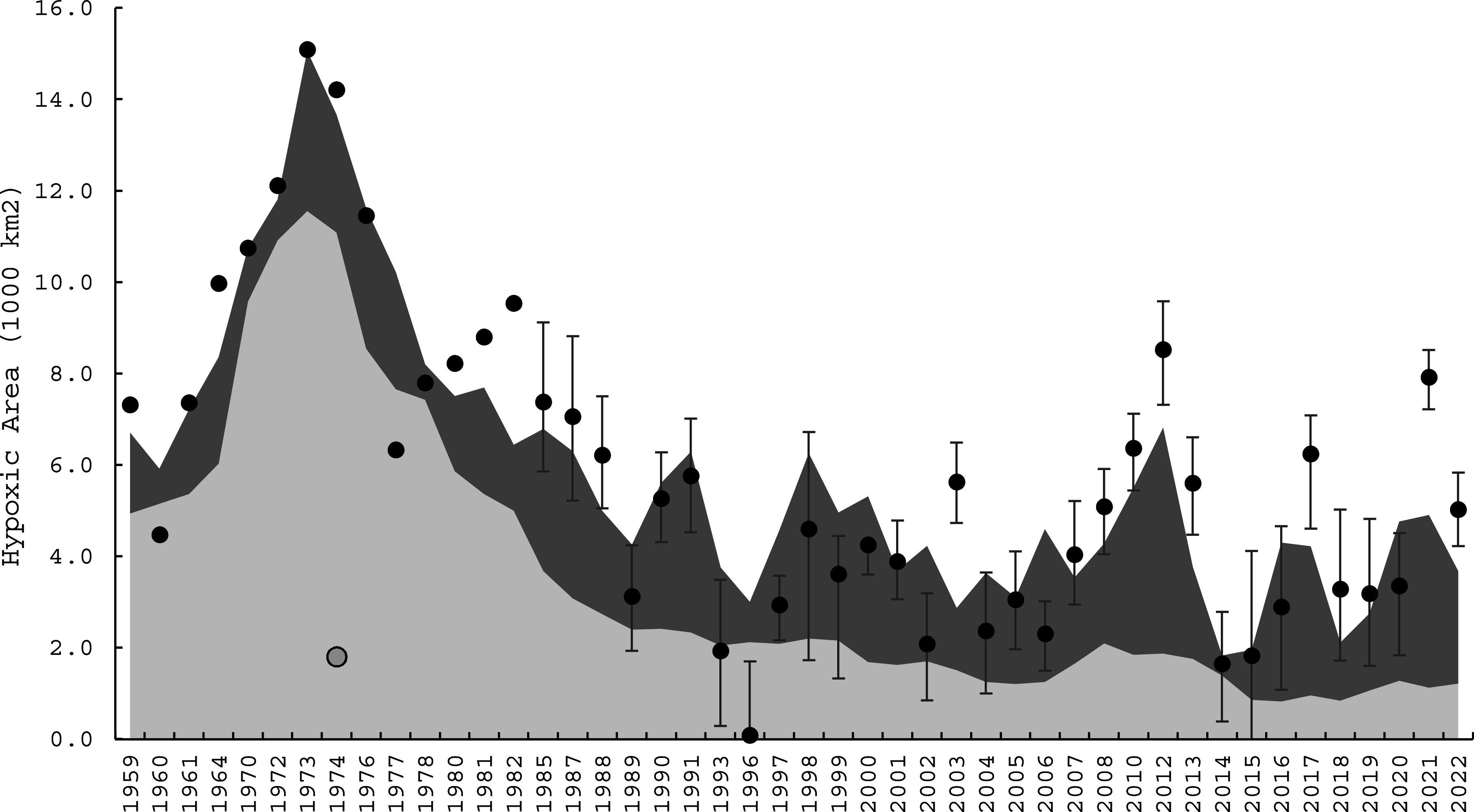
Observed (black dots) and predicted (sum of stacked areas) hypoxic extent in central Lake Erie, 1959–2022. The relative contributions of cumulative TP load (light gray) and air temperature (dark gray) are presented. An outlier year, 1975, is depicted by the gray datapoint (SI Appendix, Fig. S3). Observation error bars are from geostatistical estimates (45).

Comparing the relative contributions of TP loading and air temperature in our model illustrates that long-term hypoxia trends were driven primarily by TP loads (Figs. 2 and 3A). After the TP load reductions of the 1980s, however, interannual variability was primarily driven by air temperature (Figs. 2 and 3 and SI Appendix, Figs. S4 and S5), signifying that continued climate change can be expected to affect central Lake Erie bottom hypoxia.

Fig. 3.

(Top) Cumulative (6-y) TP load (solid black), mean March–April air temperature (dotted line), and (Fig. 2) hypoxic area (black dots), 1925–2020. (Bottom) Running average (6-y) of Lake Whitefish (thin black line), Walleye (dotted line), and Yellow Perch (dashed black line) commercial harvests and modeled hypoxia (thick black line).

Observed Variation in Hypoxic Extent.

Owing to variation in nutrient loads and temperature, we found that bottom hypoxia varied considerably during the past century (1925–2022). The 6-y cumulative TP load had a notable peak during the mid-1970s (Fig. 3A), followed by a rapid reduction through the 1980s, primarily driven by declines in Detroit River loads (SI Appendix, Fig. S4) resultant of point-source TP abatement programs (78). Over-lake air temperatures were low during the 1960s and 1970s (Fig. 3A). Combining scaled-anoxic extent during 1930–1982 with hypoxic extent estimates during 1985–2022 showed that hypoxia increased until the 1970s, with its mid-1970s peak being over triple the most recent period (1995–2022; Fig. 3A).

Observed Fisheries Harvest in Relation to TP and Hypoxia.

Commercial fishery harvests of our three focal species differentially varied with respect to nutrient-driven hypoxia. Lake Whitefish and Walleye harvests were depressed during the 1960s and 1970s, when both TP loads and hypoxic extent were high, whereas Yellow Perch harvest was highest during the same period (Fig. 3B). Statistical tests revealed significant fisheries harvest thresholds for TP load and hypoxic extent (Fig. 4 and SI Appendix, Fig. S6). Lake Whitefish appeared most negatively affected by increased TP loads and hypoxic extent, with strong harvests being rare above observed loads of 11,870 MTA (95% CI, CI = 8,790 to 17,580) and above hypoxic extents of 6,660 km² (95% CIs: 3,920 to 9,770 km²). Relative to Lake Whitefish, Walleye showed slightly higher but overlapping thresholds (TP: 12,550 MTA, CI = 9,110 to 17,290 MTA; Hypoxia: 6,700 km², 95% CIs: 4,660 to 9,630 km²). Yellow Perch showed opposite threshold effects, with weak harvests being conspicuously rare with TP loads above 10,900 MTA (95% CI: 8,790 to 15,570) and hypoxia above 5,840 km² (95% CI = 3,920 to 8,340 km²). Notably, during 1991–2020, reduced TP loads and bottom hypoxia appear to have benefited Walleye and negatively affected Yellow Perch, with Lake Whitefish harvests remaining low despite water quality returning to levels that once favored strong harvests (Fig. 4 and SI Appendix, Fig. S6).

Fig. 4.

Commercial harvests of Lake Whitefish (Top), Walleye (Middle), and Yellow Perch (Bottom) in Lake Erie (1000s of kg, round weight) as a function of 5-y running means of simulated hypoxic extent (1000s of km²; Left) and reconstructed cumulative TP loading (1000s of metric tons annually; Right), 1932–2020. Dashed vertical lines represent the best threshold in each panel (all P < 0.0001), with the rectangle indicating the upper and lower 95% CI around the mean threshold (SI Appendix).

Impact of Current TP Loading Target on Hypoxia and Fisheries.

To reduce hypoxic extent, the binational GLWQA (82) set the central basin TP load reduction target to 40% of the 2008 load (9,100 MTA). This load was chosen to maintain summer mean hypolimnetic DO above 2 mg/l and hypoxic extent below 2,500 km² (80). Our model (SI Appendix, Fig. S3) predicts that reducing TP loads by 40% would result in a mean hypoxic extent of 2,000 km², a level between the 2,500 km² target and the 1930 extent (1,500 km²) that has been characterized by low productivity akin to presettlement conditions (88–90) and suboptimal fishery harvests for Walleye and Yellow Perch (Fig. 4). Importantly, our modeling indicates that a 2,500 km² extent would, on average, require only a 33% (not 40%) TP load reduction from 2008.

Regardless, both the 33% and 40% TP load reduction appear more restrictive than necessary to support contemporary fishery harvests. Taking a precautionary approach, we used the lower 95% CIs from our threshold analyses (Fig. 4 and SI Appendix, Fig. S6) to estimate the impacts of altered nutrient loading on Lake Erie’s fisheries. Our analyses showed that hypoxic extents below ~4,700 km² and ~3,900 km² appear sufficient to offer the potential for high Walleye and Lake Whitefish harvests, respectively. According to our model under current climate conditions, maintaining hypoxic extent below ~4,300 km² (the mean of the lower 95% CIs for Walleye and Lake Whitefish thresholds) on average would require only a 7% reduction from the 2008 TP load, much less than the current 40% target reduction. This lower reduction target would also be more protective of the Yellow Perch fishery given that harvests appear to benefit from high TP loads and do not appear limited by bottom hypoxia (Fig. 4 and SI Appendix, Fig. S6). However, because projected climate warming, even as soon as 2030–2059, is expected to increase bottom hypoxia (e.g., refs. 29, and 91–93; below), a 7% TP load reduction is unlikely to be appropriate for the future.

Projected Impacts of Climate Change on Hypoxia and Fisheries.

Lag times of impacts on nutrient export from watersheds range from years to decades owing to land use changes taking years to implement, as well as watershed retention (e.g., refs. 94–97) and internal cycling of lake P (98, 99). Thus, the results of land management actions (e.g., agricultural conservation practices) will play out on climatic timescales.

Substantial interannual variability in hypoxia has been driven by air temperature, especially during recent years when TP loads have been more stable and interannual variability in spring temperatures has been more variable (Fig. 3 and SI Appendix, Figs. S4 and S7). Thus, climate warming is expected to increase hypoxia and potentially offset TP abatement efforts. While both air and water temperatures increased during 1985–2022 (SI Appendix, Fig. S7), we did not find a statistically significant change in hypoxic area during 1985–2022, perhaps because TP load gradually declined. Even so, our modeling showed that a 710 km² increase in hypoxic area occurred for every 1 °C increase in mean March–April air temperature. We also found that both mean hypoxic thickness and volume increased after a change-point (100) detected around 1996 (SI Appendix, Fig. S7). Likewise, hypoxic duration, which was historically confined to August and September, has expanded to July and October in some years after 2010 (SI Appendix, Fig. S7).

Given that continued warming is expected to directly affect thermal stratification, causing it to occur earlier and last longer (101, 102), we explored how warming might impact future hypoxic extent and fishery harvests. Using output from 15 CMIP6 climate models and three greenhouse gas mitigation pathways (SI Appendix) to modify temperatures in our hypoxia model, we learned that the TP load reduction required to achieve the hypoxia target will increase through time (Fig. 5). For example, under the climate mitigation pathway most like the path we are currently on (SSP2-4.5), we projected that 80% of the time a 7% reduction from the 2008 load would result in hypoxic areas less than 7,100 km² and 7,900 km² by mid- and late century. Protecting Walleye and Lake Whitefish harvests by keeping hypoxic area below 4,000 km² 80% of the time (Fig. 4) would require TP loading reductions of 55% by midcentury. A less aggressive greenhouse gas mitigation scenario (SSP5-8.5) would require 60% reductions, and an even the more aggressive mitigation scenario (SSP1-2.6) would still require 51% reductions (Table 1 and SI Appendix, Fig. S8). Importantly, while implementing 50 to 60% load reductions under future climates would support the potential for high Walleye and Lake Whitefish commercial harvests, they would come at the expense of the Yellow Perch commercial fishery, owing to its dependency on high nutrient inputs.

Fig. 5.

(Top) Hypoxic extent as a function of mean March–April air temperature. Mean hypoxic extent (thick, ascending black line) and upper and lower 60% prediction intervals (thinner, ascending gray lines) for a 7% reduction in TP loads relative to 2008. Vertical lines represent current (1992–2022; solid), mid-century (2030–2059; dashed), and late-century (2060–2099; dotted) temperature conditions for the middle-of-the-road (SSP2-4.5) greenhouse gas emission scenario. Hypoxic values at the upper prediction interval are met 80% of the time. Precautionary hypoxia thresholds (lower 95% CI, per Fig. 4) for Walleye (horizontal solid line) and Lake Whitefish (horizontal dashed line). (Bottom) Percent TP load reduction required to meet the hypoxia target on average (solid ascending line) and 80% of the time (dashed ascending line) at the mid- and late century. Results for the sustainable development (SSP1-2.6) and no additional climate policy (SSP5-8.5) scenarios are presented in SI Appendix, Fig. S8.

Table 1.

Lake Erie hypoxic extent and required TP load reductions under current conditions and three future greenhouse gas emission scenarios (SSP2: middle of the road; SSP1: sustainable development; SSP5: no additional climate policy) during midcentury (2030–2059) and late century (2060–2099)

		Projected hypoxic area with a 7% load reduction from 2008		Percent reduction from 2008 needed for hypoxia <4,000 km2
		Mean	80% of the time	Mean	80% of the time
Climate mitigation pathway	Current climate	4,000	5,800	8%	35%
SSP2	Midcentury	5,300	7,100	27%	55%
	Late century	6,000	7,900	39%	68%
SSP1	Midcentury	4,900	6,800	22%	51%
	Late century	5,200	7,100	26%	55%
SSP5	Midcentury	5,500	7,400	31%	60%
	Late century	7,500	9,400	62%	91%

Discussion

To help facilitate management decision-making in ecosystems experiencing bottom hypoxia, we calibrated a predictive model of Lake Erie hypoxia that allowed us to delineate the relative importance of nutrient loading and temperature as drivers of hypoxia and reconstruct hypoxic extent during the past century such that we could quantify its impact on the harvest dynamics of three important fisheries. Beyond showing how nutrient inputs and temperature in large freshwater ecosystems can interact to drive long-term hypoxia dynamics, as well as why climate change needs to be considered when setting nutrient-management targets, we demonstrated how management plans designed to mitigate hypoxia can lead to water quality–fisheries tradeoffs that complicate management. Given that both freshwater and marine ecosystems worldwide are experiencing hypoxia and climate warming, our study findings and approach can help agencies both anticipate and navigate the wicked landscape of nutrient management decision-making, as well as understand why adaptive EBM is vital to sustaining valued societal services in ecosystems experiencing human-driven stress.

Hypoxia Drivers.

Our modeling showed that climate variation has become an important driver of hypoxic extent during recent decades. The large increase in hypoxia during 1960–1975 and subsequent rapid decrease through the 1980s were driven primarily by changes in the cumulative TP load (Fig. 3). This influence of cumulative TP load is consistent with long-term “memory” effects observed in other lakes and the potentially large flux of P from central basin sediments (98, 99, 103, 104), and is supported by empirical measurements (105) and modeling output from Lake Erie (106, 107). The lower and relatively constant hypoxic extent after the 1990s tracks the slower decline in TP loads, with interannual variability since 1996 being controlled primarily by air temperature, which has increased the strength and duration of stratification while lowering the DO saturation concentration (29, 53, 56, 92, 108). This secondary control of bottom hypoxia by meteorology also is well documented in other freshwater and marine ecosystems (e.g., refs. 109–111), indicating that climate change must be considered in water quality planning and management.

Increased hypoxic extent after the mid-1990s has been attributed to re-eutrophication, consistent with increased dissolved P loads and HABs in the western basin (e.g., refs. 46, 50 and 106). However, our extended dataset allowed us to learn that small hypoxic extents (e.g., 1993–1997) are more likely related to the low temperatures and delayed summer stratification than TP loads (i.e., temperatures during these years were below the long-term mean; see SI Appendix, Fig. S5). The dependence of bottom hypoxia on temperature has been previously suggested for Lake Erie (112), as well as in other freshwater and marine ecosystems (e.g., refs. 92, 109, 110 and 113). This finding highlights the value of long-term monitoring data, exploring multiple drivers when attributing causal mechanisms of hypoxia, and periodically reassessing modeling predictions.

While the impact of climate change on nonpoint source (watershed) TP loading into Lake Erie remains unresolved due to potentially opposing effects of increased evapotranspiration and precipitation (30, 114), continued warming is expected to increase bottom hypoxia and anoxia (53, 54, 91–93). Our modeling supported this prediction with hypoxia thickness, volume, and duration increasing as temperature increased. Our results are consistent with those from other ecosystems, including Chesapeake Bay, United States (110), the northern Gulf of Mexico, United States (115), Lake of Zurich, Switzerland (92), Blelham Tarn, United Kingdom (91), and Lake Fuxian, China (93). Collectively, these studies and our modeling indicate that continued climate change holds the potential to offset impending efforts to reduce hypoxia in freshwater and marine ecosystems alike.

Hypoxia Thresholds and Water Quality–Fisheries Tradeoffs.

Documented bottom–up effects of increased nutrients on prey availability have validated the ascending portion of the unimodal nutrient-fish productivity curve (e.g., ref. 38). However, long-term consequences of bottom hypoxia on fisheries yield have remained elusive in most freshwater and marine ecosystems (39–41) due partly to a lack of long-term historical DO data. Herein, we demonstrated a direct quantitative relationship between bottom hypoxia and commercial fisheries harvest monitoring data during the past century (1932–2022). We also showed that reducing TP inputs to mitigate bottom hypoxia can be expected to cause tradeoffs in fisheries harvests, with some species “winning” under TP abatement (e.g., Lake Whitefish and possibly Walleye), and others “losing” (e.g., Yellow Perch).

While our threshold relationships between fisheries harvest and hypoxic extent are correlative, they hold even after accounting for potential confounding effects on fisheries harvest, including invasive species and climate variation (SI Appendix, Figs. S9–S16). They (and their resultant tradeoffs) are also supported by knowledge of each species physiological tolerances and habitat needs. Lake Whitefish is expected to be highly limited by bottom hypoxia because of its dependence on cold temperatures found only in bottom waters during summer and on benthic macroinvertebrates as prey (59, 116). Lost access to benthic thermal habitat and prey can negatively affect foraging and population growth of coregonines (e.g., refs. 63, 64 and 117) and has been implicated in reduced Lake Whitefish fitness and recruitment to the fishery in Lake Erie (10, 57, 59). Conversely, benthic omnivores like Yellow Perch, which are tolerant of warmer water and capable of feeding on planktonic prey as juveniles and adults, can persist during hypoxia by residing in areas above the hypoxic zone or in oxygenated nearshore waters (58, 60, 62). Such species will be less hampered by hypoxia than Lake Whitefish if sufficient pelagic prey (e.g., zooplankton) is abundant. Species with intermediate thermal tolerances and that are not facultative benthivores, such as piscivorous Walleye, would be expected to show an intermediate response, as reduced access to cool bottom waters could be offset by potentially increased access to prey fish that aggregate at the edges of the hypoxia zone (118). These species-specific tolerances to hypoxia and flexibility in feeding and habitat use help explain why coregonines like Lake Whitefish tend to decline with eutrophication and are succeeded by more tolerant species such as Walleye and eventually Yellow Perch (119, 120).

Our modeling suggests that the degree to which such tradeoffs occur in Lake Erie will ultimately depend on management targets (e.g., achieving the 4,000 km² hypoxia threshold on average vs. 80% of the time), given that the targets could potentially be above or below the hypoxia thresholds identified for our three focal species. These varied responses to hypoxia highlight the need for fisheries management to consider species-specific thresholds and be adaptive when setting quotas and managing their constituents.

While our study focused on three specific Lake Erie fishes, their collective response to nutrient- and climate-driven hypoxia is relevant to other aquatic ecosystems. Each of these species is of ecological, cultural, and economic importance and exhibits life-history traits similar to commercially exploited fishes found in other large aquatic ecosystems, including marine systems (121, 122). Additionally, these species span a wide range of thermal tolerance and sensitivity to bottom hypoxia, which is typical of fish communities residing in other freshwater and marine ecosystems (123–125). And the behavioral and demographic responses of our three species to hypoxia are like those observed in other hypoxia-sensitive freshwater and marine fishes (13, 42, 43, 66, 67, 126). Similar fisheries tradeoffs are therefore expected to occur in other ecosystems as nutrients are managed to mitigate bottom hypoxia and climate change continues [e.g., Baltic Sea: (111, 127); Chesapeake Bay: (110, 128); Northern Gulf of Mexico: (109, 129)].

Management Implications.

Our analysis offers important insights into the impact of hypoxia on three culturally, ecologically, and economically important fishes: Lake Whitefish, Walleye, and Yellow Perch. While other factors also contributed to the decline of Lake Whitefish and Walleye leading up to the peak eutrophication period in Lake Erie during the 1960s and 1970s [e.g., overharvest, invasive species; (57, 130); and SI Appendix, Figs. S9–S16], we view bottom hypoxia as an important environmental change that has negatively influenced commercial harvests. This view supports previous, more speculative studies that could not quantitatively relate hypoxia to harvest levels (10, 57, 59) because of an absence of long-term DO data and is relevant to the myriad of other aquatic ecosystems worldwide that are facing multiple stressors, including climate change and bottom hypoxia.

Collectively, our findings highlight the need for fishery management to acknowledge changing ecosystem conditions, especially those brought on by nutrient management and climate change. As is the case in most other large lake and coastal marine ecosystems experiencing anthropogenic environmental change (31–34, 131), Lake Erie has been nonstationary and is likely to remain that way with continued climate change (110, 132, 133). Such nonstationarity, whether due to planned management actions (e.g., nutrient abatement, fishery harvest) or unplanned perturbations (e.g., climate change, invasive species), reaffirms the need for management agencies in both freshwater and marine ecosystems to be flexible and adaptive.

This same lesson applies to water quality management. While a less stringent TP reduction target under the current climate should be considered, its effectiveness might be short-lived in a future climate. This same conclusion has been drawn in coastal marine ecosystems where bottom hypoxia is mostly controlled by nitrogen inputs (109–111, 127–129). Thus, nutrient management planners also need to be receptive to new modeling forecasts and be willing and prepared to modify ongoing strategies. Patience will also be required as it may take many years to implement significant land-use changes, followed by long lag times for watershed loads to respond, and additional time for the lake to respond. The fact that results of management actions are likely to play out over multidecadal periods, which matches observations in other aquatic ecosystems (e.g., refs. 134, and 135), with climate change being an important mediating factor (101, 102, 109–111, 127–129, 136), reinforces the value of adaptive EBM strategies.

If done well, adaptive EBM ensures the needed updating and reevaluating of models used to make forecasts with new data (sensu refs. 26, and 27), which can lead to more reliable identification and evaluation of management targets and tradeoffs (19, 20, 76). In addition, because stakeholder and rightsholder expectations of water quality and fisheries production can shift with changing ecosystem conditions (137, 138), adaptive EBM plans that consider their perceptions and values (18, 19) can help secure plan buy-in, which is key to successful implementation (24). Such buy-in is critical, given that the fishery-water quality tradeoffs shown herein, along with the human health issues from HABs and concerns of the agriculture industry over TP load reduction targets (139), create a wicked management landscape. Successful use of adaptive EBM, like what is being called for inside (24, 86, 87) and outside of the Great Lakes Basin (19, 140–142), can provide a means to identify, understand, and navigate wicked management dilemmas both now and in the face of future human-driven environmental change and help keep the many services that our ecosystems provide sustainable.

When developing models to support adaptive EBM efforts, we encourage the use of simple models akin to what was used herein. While complex models like Ecopath with Ecosim and Atlantis are being increasingly used to support aquatic ecosystem management, and do have their benefits (143, 144), their use in management decision-making has been limited because of inflexible management structures that are ill-equipped to handle new, more complex outputs, undertrained staff that cannot run or interpret output, and the fear of setting a new precedent among other things (144). The use of simpler models that are more understandable and easily modified, like whose used herein, should be considered as an alternative or complementary approach, which may increase their use in management.

Future Directions.

One of the key findings of our work is that warming associated with climate change exacerbates hypoxia and will continue to do so in the future. The other primary factor in our model is nutrient loading. Studies have shown that nutrient export is itself sensitive to temperature and precipitation changes resulting from climate change (e.g., refs. 28, 30, 95, 96, and 145). In some cases, increased evapotranspiration caused by warmer temperatures and less snowpack may partially or even fully offset the effects of increased precipitation (30, 114). However, other studies suggest that increased precipitation-driven discharge under a warming climate may increase nutrient loads from tributaries in Lake Erie (146) and in the northern Gulf of Mexico (129). These factors were not included in our model but incorporating them as part of future work would make it possible to further refine projections of hypoxia under future climate conditions.

Opportunities also exist with respect to modeling fisheries responses, which are relevant to developing adaptive EBM plans in Lake Erie and beyond. Herein, we focused on the role of hypoxia in driving variation in fishery harvests. However, invasive species, variation in exploitation and harvest levels, and changes in thermal conditions also influenced recruitment to the commercial fisheries of all three species during the past century (57, 133, 147–149), with their effects likely most evident during years with low hypoxic extent (i.e., small hypoxic extents provide the potential for high fishery harvests but do not guarantee them). For example, climate-induced reductions in ice cover, which are expected to reduce Lake Whitefish survival during the egg and larval stage (149, 150), could explain why harvest of this species has not achieved high levels like those prior to the 1960s (despite their being ample TP; Fig. 4). Similarly, while hypoxia can limit Yellow Perch foraging and growth habitat in Lake Erie (58, 60), reduced watershed inputs of TP that limit zooplankton production (151) appear to be a stronger driver of fishery dynamics (Fig. 4). These complexities point to the need to consider more than the influence of hypoxia on fisheries dynamics. For example, adding a predictor variable that accounts for the impact of climate change on thermal habitat, predator abundance, and prey availability (147, 148, 152–154) could further enhance forecasts of nutrient-driven changes in hypoxia on fishery yields, and allow for interactive effects of these stressors to be assessed, while keeping the overall model simple enough for others less adept at modeling to understand and use. Clearly, this suggestion is applicable to any ecosystem experiencing multiple anthropogenic stressors, such as eutrophication-driven hypoxia and climate change.

Conclusions

Results presented herein reveal useful insights that can benefit nutrient management decision-making on Lake Erie, with important implications for other aquatic systems worldwide. Our study demonstrates a simple, general approach that could be adapted to other ecosystems to help agencies navigate the wicked management landscape posed by multisector management in a nonstationary ecosystem. By updating an existing hypoxia model with newer data, we were able to fill gaps in the historical record and then tie this record to historical fishery harvest data to provide a clear, unique illustration of how hypoxia has negatively impacted key fisheries over a multidecadal period. Our approach also allowed us to identify TP loading and hypoxic extent thresholds above which some key fisheries species were negatively impacted.

Interestingly, not all species responded negatively to hypoxic conditions as they were differentially limited by reduced nutrient loading. This finding illustrates the need for nutrient management decision-makers to consider potential fisheries tradeoffs when mitigating water quality impairments such as hypoxia. The simple nutrient-temperature-hypoxia and hypoxia-fisheries models used herein allowed us to quantitatively assess the efficacy of current management nutrient targets under current and future climates. Importantly, we showed for Lake Erie that current nutrient load reduction targets are likely overly restrictive from the perspective of fishery needs, but that those reductions—and likely more—appear necessary as the climate continues to warm. This result aligns with hypoxia modeling studies conducted in other coastal ecosystems (e.g., Baltic Sea, Chesapeake Bay, northern Gulf of Mexico), although an extension to fisheries in those ecosystems was not found.

Finally, our study demonstrates the advantage of considering multiple ecosystem sectors/services (e.g., water quality and fisheries) when developing management plans for nonstationary ecosystems experiencing anthropogenic change and highlights how adaptive EBM approaches that are supported by simple, updated models can help inform future management decision-making. With the continued growth of such approaches, we expect the ability of agencies to understand and successfully navigate the complex landscape created by management decision-making and continued human-driven environmental change to increase, which will go a long way to protecting the many services that our ecosystems provide to society.

Methods

Bottom Hypoxia.

Areal hypolimnetic hypoxic extent estimates with uncertainty bounds generated via Monte Carlo simulations were derived from DO profiles collected from 10 fixed stations in the offshore waters of the central basin, sampled at approximately 3-wk intervals between June and October, 1985–2022, by the U.S. Environmental Protection Agency, augmented with samples from Environment and Climate Change Canada and the National Oceanic and Atmospheric Administration (NOAA), as described by Zhou et al. (45). The hypoxic extent conditional realizations from individual cruises were first averaged within early and late seasons, and the resulting estimates were averaged between the early and late season to create an estimate of the seasonally averaged hypoxic extent and its uncertainty. Seasonally averaged hypoxic extent estimates were therefore obtained for all years for which at least one cruise is available during both the early and late season (resulting in the exclusion of 1986, 1992, 1994, 1995, 2009, and 2011). We also used these profiles to estimate the thickness of the hypoxic layer by determining the depth at which DO fell below 2 mg/l from each vertical profile. We then multiplied the average thickness for each date with the associated areal extent to estimate hypoxic volume.

Anoxic area was determined (along with hypoxic area) for each sampling date (1985–2022, n = 151) using a bottom-water DO threshold of 0.5 mg/L, the same value used by Herdendorf [(44); pers. comm.]. We converted anoxic area from before 1985 (44) to hypoxic area using a least-squares regression relationship between the hypoxic/anoxic ratio (h) and anoxic extent (A): h = 3.241A^−0.365 (n = 151, R² = 0.95).

Temperature.

Mean monthly over-lake air temperatures for 1950–2023, used as input to the hypoxia model (see below), were provided by the U.S. Army Corps of Engineers (D. Fielder, USACE, personal communication), developed using the approach of Hunter et al. (155). March–April over-lake average air temperature (y) before 1950 was predicted from a least-squares regression model (y = –0.332 + 0.718x; R² = 0.74) with March–April average air temperature (x) at the National Weather Service station (Fig. 1, USW00014860). Daily water and air temperatures, obtained from National Data Buoy Center, buoy 45005 (156) were also used to assess recent climate trends.

TP Loading Estimates.

We used the Detroit, Maumee, Raisin, Cuyahoga, and Sandusky rivers (DRT) as surrogates for the water-year TP load into the central basin (Fig. 1). To be consistent with GLWQA targets and other efforts, we divided our TP estimates by 0.78 (SD = 0.017), which is the 2003–2013 average ratio of these loads to the total central basin load (157).

1960–2022 Tributary Loads.

Daily TP loading estimates start in 1974 for the Sandusky River, in 1975 for the Maumee, 1981 for the Cuyahoga, and 1982 for the Raisin (158). Daily loads for these periods were calculated by multiplying the daily flow-weighted mean TP concentration (FWMC) by daily United States Geological Survey (USGS) flow for each river. In the instance of missing data (<5% of the time), daily FWMCs were interpolated from previous days (159). We estimated daily loads from 1960 to the onset of monitoring for each river using relationships between daily discharge and TP load or FWMC from the first 3 y of monitoring. More specifically, the first 3 y of each monitoring period for each river were separated into three hydrologically important periods: March–June, July–October, and November–February. Linear relationships were developed for log₁₀-load vs. log₁₀-flow and polynomial relationships for log₁₀-FWMC vs. log₁₀-flow for each season. The estimated daily concentration, calculated as the average of the two approaches, was multiplied by observed daily USGS flow for each river.

1967–2022 Detroit River.

Detroit River loads for 1967–1974 came from Fraser (160). The loads for 1975–1981 were averages of estimates by Fraser (160) and Yaksich et al. (161). Estimates for 1982–1997 were based on linear interpolation of FWMC and discharge from the USGS gage at Ft. Wayne (#04165710). Loads for 1998–2022 were estimated by adding loads leaving Lake St. Clair to those entering the Detroit River (following ref. 162).

1922–2022 Total Load.

Estimates of TP load into the central basin during 1922–1967 came from Chapra (163), based on transfer coefficients associated with the 1) sewered population; 2) runoff from agricultural, urban, and forested areas; and 3) and the atmosphere. These estimates explained 7% of the variability of loads across the Great Lakes basin. When used as input to a mass-balance model, they explained 88% of the TP concentration variability across the five lakes. We calculated the 1967–2022 estimates by summing the DRT loads, scaled per above.

Fisheries Data.

No fisheries-independent data or harvest-per-unit-effort data exist in Lake Erie before 1969. Thus, we used total annual commercial harvests (kg, round weight) of Lake Whitefish, Walleye, and Yellow Perch during 1928–2020 as our proxy for fisheries production. Data came from GLFC (164) and were corrected to account for changes in harvest regulations among jurisdictions and reporting tendencies through time, following Sinclair et al. (12). Additionally, as demonstrated by Sinclair et al. (12), the commercial harvest of each species tracked estimated indices of abundance and population size, as well as known historical responses of each species to eutrophication, during recent decades.

Hypoxia Model.

Our predictive model of hypoxic extent expands the model developed by Del Giudice et al. (29). That model predicted hypoxic extent for 30 y between 1985 and 2015 as a function of the cumulative TP load from four tributaries (without the Detroit River) from the previous 9 y and average March–April air temperature. The latter term was used as a surrogate representing increased surface temperatures, lengthened and strengthened stratification, increased algal production and sedimentation, and reduced transport of DO to the hypolimnion (29). We expanded the model by adding Detroit River loads and increasing the calibration dataset from 25 to 53 y (as available, from 1959 to 2022).

Model development and testing.

We calibrated our model using observed mean summertime hypoxic extent, which is when bottom hypoxia has been most severe in central Lake Erie. We developed a Bayesian multiple linear regression model using the rstanarm package (165) in R (166) with Stan (167) to predict hypoxic area from the cumulative TP load and the spring air temperature (SI Appendix). We tested model robustness using leave-one-out cross-validation where each year’s observation was predicted after recalibrating the model to a reduced dataset where the observation from the forecast year was removed. We also conducted pseudoblind forecasts to test the model when calibrated only to the observations from previous years by calibrating the model with observations from 1959 to the year preceding the forecast year. This process was repeated for 1970–2022.

Response curves.

Producing annual forecasts of hypoxic area from cumulative TP load and spring air temperature is straightforward when both types of data exist. For future conditions in which air temperature is unknown, we developed a TP load-response curve based on 10,000 Monte Carlo simulations with air temperature drawn from a normal distribution fit to observed data during 1992–2022 (mean = 3.4, SD = 1.46) and adding the resulting variances to model parameter and residual error variance. Doing so allowed us to quantify 95% prediction intervals (CIs), as well as more policy-relevant 60% CIs where the upper CI represents reaching a specific hypoxic extent 80% of the time.

Climate forecasts.

For future climate scenarios, we used temperature forecasts from 15 models with three socioeconomic pathways listed in Fig. 5 (168). To do so, we increased the air temperature distribution in the Monte Carlo simulations above current conditions (2012–2022) with distribution increments between CMIP6 current distributions and those for mid-century (2030–2059) and late-century (2070–2099) projections (SI Appendix).

Fisheries Response to Loads and Hypoxia.

To quantify the response of Yellow Perch, Walleye, and Lake Whitefish commercial harvests to hypoxic extent and TP loads during 1925–2020, we used two-dimensional Kolmogorov–Smirnov tests (2dKS; 169). These tests allowed us to identify the existence of any thresholds (with 95% CIs) in hypoxic extent and TP load four each species, above which or below which harvest distributions changed (SI Appendix, Fig. S6).

Supplementary Material

Appendix 01 (PDF)

Data, Materials, and Software Availability

All data used in the analysis are now included in the supporting information. The data used in the fisheries modeling was included as the last table in this document, which has been uploaded here.

References

- 1.Vitousek P. M., Mooney H. A., Lubchenco J., Melillo J. M., Human domination of Earth’s ecosystems. Science 277, 494–499 (1997). [Google Scholar]
- 2.Díaz S., et al. , Pervasive human-driven decline of life on earth points to the need for transformative change. Science 366, eaax3100 (2019). [DOI] [PubMed] [Google Scholar]
- 3.Paine R. T., Tegner M. J., Johnson E. A., Compounded perturbations yield ecological surprises. Ecosystems 1, 535–545 (1998). [Google Scholar]
- 4.Carpenter S. R., et al. , Nonpoint pollution of surface waters with phosphorus and nitrogen. Ecol. Appl. 8, 559–568 (1998). [Google Scholar]
- 5.Smith S., et al. , River nutrient loads and catchment size. Biogeochemistry 75, 83–107 (2005). [Google Scholar]
- 6.Cloern J. E., Our evolving conceptual model of the coastal eutrophication problem. Mar. Ecol. Prog. Ser. 210, 223–253 (2001). [Google Scholar]
- 7.Smith V. H., Joye S. B., Howarth R. W., Eutrophication of freshwater and marine ecosystems. Limnol. Oceanogr. 51, 351–355 (2006). [Google Scholar]
- 8.Blann K. L., Anderson J. L., Sands G. R., Vondracek B., Effects of agricultural drainage on aquatic ecosystems: A review. Crit. Rev. Environ. Sci. Technol. 39, 909–1001 (2009). [Google Scholar]
- 9.Stockner J., Rydin E., Hyenstrand P., Cultural oligotrophication: Causes and consequences for fisheries resources. Fisheries 25, 7–14 (2000). [Google Scholar]
- 10.Ludsin S. A., Kershner M. W., Blocksom K. A., Knight R. L., Stein R. A., Life after death in Lake Erie: Nutrient controls drive fish species richness, rehabilitation. Ecol. Appl. 11, 731–746 (2001). [Google Scholar]
- 11.Jeppesen E., et al. , Lake responses to reduced nutrient loading—An analysis of contemporary long-term data from 35 case studies. Freshwater Biol. 50, 1747–1771 (2005). [Google Scholar]
- 12.Sinclair J., Fraker M., Hood J., Reavie E., Ludsin S., Eutrophication, water quality, and fisheries: A wicked management problem with insights from a century of change in Lake Erie. Ecol. Soc. 28, 10 (2023). [Google Scholar]
- 13.Caddy J., Toward a comparative evaluation of human impacts on fishery ecosystems of enclosed and semi-enclosed seas. Rev. Fish. Sci. 1, 57–95 (1993). [Google Scholar]
- 14.Whittier T. R., Hughes R. M., Evaluation of fish species tolerances to environmental stressors in lakes in the northeastern United States. North Am. J. Fish. Manage. 18, 236–252 (1998). [Google Scholar]
- 15.Slocombe D. S., Implementing ecosystem-based management. BioScience 43, 612–622 (1993). [Google Scholar]
- 16.Berkes F., Implementing ecosystem-based management: Evolution or revolution? Fish. Fish. 13, 465–476 (2012). [Google Scholar]
- 17.Link J. S., Marshak A. R., Ecosystem-Based Fisheries Management: Progress, Importance, and Impacts in the United States (Oxford University Press, 2021). [Google Scholar]
- 18.Leslie H. M., McLeod K. L., Confronting the challenges of implementing marine ecosystem-based management. Front. Ecol. Environ. 5, 540–548 (2007). [Google Scholar]
- 19.Levin P. S., Fogarty M. J., Murawski S. A., Fluharty D., Integrated ecosystem assessments: Developing the scientific basis for ecosystem-based management of the ocean. PLoS Biol. 7, e1000014 (2009). [DOI] [PMC free article] [PubMed] [Google Scholar]
- 20.Tallis H., et al. , The many faces of ecosystem-based management: Making the process work today in real places. Mar. Policy 34, 340–348 (2010). [Google Scholar]
- 21.Birgé H. E., Allen C. R., Garmestani A. S., Pope K. L., Adaptive management for ecosystem services. J. Environ. Manage. 183, 343–352 (2016). [DOI] [PMC free article] [PubMed] [Google Scholar]
- 22.Doswald N., et al. , Effectiveness of ecosystem-based approaches for adaptation: Review of the evidence-base. Clim. Dev. 6, 185–201 (2014). [Google Scholar]
- 23.Lindegren M., Brander K., Adapting fisheries and their management to climate change: A review of concepts, tools, frameworks, and current progress toward implementation. Rev. Fish. Sci. Aquacult. 26, 400–415 (2018). [Google Scholar]
- 24.Ludsin S. A., et al. , A perspective on successful implementation of ecosystem-based approaches to management and conservation in the Laurentian Great Lakes. Aquat. Ecosyst. Health Manage. 27, 9–26 (2024). [Google Scholar]
- 25.Boesch D. F., Scientific requirements for ecosystem-based management in the restoration of chesapeake bay and coastal louisiana. Ecol. Eng. 26, 6–26 (2006). [Google Scholar]
- 26.Myers R. A., When do environment–recruitment correlations work? Rev. Fish Biol. Fish. 8, 285–305 (1998). [Google Scholar]
- 27.Tamburello N., Connors B. M., Fullerton D., Phillis C. C., Durability of environment–recruitment relationships in aquatic ecosystems: Insights from long-term monitoring in a highly modified estuary and implications for management. Limnol. Oceanogr. 64, S223–S239 (2019). [Google Scholar]
- 28.Michalak A. M., et al. , Record-setting algal bloom in lake erie caused by agricultural and meteorological trends consistent with expected future conditions. Proc. Natl. Acad. Sci. U.S.A. 110, 6448–6452 (2013). [DOI] [PMC free article] [PubMed] [Google Scholar]
- 29.Del Giudice D., Zhou Y., Sinha E., Michalak A. M., Long-term phosphorus loading and springtime temperatures explain interannual variability of hypoxia in a large temperate lake. Environ. Sci. Technol. 52, 2046–2054 (2018). [DOI] [PubMed] [Google Scholar]
- 30.Zhao G., Merder J., Ballard T. C., Michalak A. M., Warming may offset impact of precipitation changes on riverine nitrogen loading. Proc. Natl. Acad. Sci. U.S.A. 120, e2220616120 (2023). [DOI] [PMC free article] [PubMed] [Google Scholar]
- 31.Crain C. M., Kroeker K., Halpern B. S., Interactive and cumulative effects of multiple human stressors in marine systems. Ecol. Lett. 11, 1304–1315 (2008). [DOI] [PubMed] [Google Scholar]
- 32.Hewitt J. E., Ellis J. I., Thrush S. F., Multiple stressors, nonlinear effects and the implications of climate change impacts on marine coastal ecosystems. Global Change Biol. 22, 2665–2675 (2016). [DOI] [PubMed] [Google Scholar]
- 33.Steinman A. D., et al. , Ecosystem services in the great lakes. J. Great Lakes Res. 43, 161–168 (2017). [DOI] [PMC free article] [PubMed] [Google Scholar]
- 34.Jenny J.-P., et al. , Scientists’ warning to humanity: Rapid degradation of the world’s large lakes. J. Great Lakes Res. 46, 686–702 (2020). [Google Scholar]
- 35.Friedland K. D., et al. , Pathways between primary production and fisheries yields of large marine ecosystems. PLoS ONE 7, e28945 (2012). [DOI] [PMC free article] [PubMed] [Google Scholar]
- 36.Oglesby R. T., Relationships of fish yield to lake phytoplankton standing crop, production, and morphoedaphic factors. J. Fish. Board Can. 34, 2271–2279 (1977). [Google Scholar]
- 37.Downing J. A., Plante C., Lalonde S., Fish production correlated with primary productivity, not the morphoedaphic index. Can. J. Fish. Aquat. Sci. 47, 1929–1936 (1990). [Google Scholar]
- 38.Hessen D. O., Faafeng B. A., Brettum P., Andersen T., Nutrient enrichment and planktonic biomass ratios in lakes. Ecosystems 9, 516–527 (2006). [Google Scholar]
- 39.Chesney E. J., Baltz D. M., “The effects of hypoxia on the northern Gulf of Mexico coastal ecosystem: A fisheries perspective” in Coastal Hypoxia: Consequences for Living Resources and Ecosystems, Rabalais N. N., Turner R. E., Eds. ( American Geophysical Union, Coastal and Estuarine Studies, 2001), vol. 58, pp. 321–354.
- 40.Breitburg D. L., Hondorp D. W., Davias L. A., Diaz R. J., Hypoxia, nitrogen, and fisheries: Integrating effects across local and global landscapes. Annu. Rev. Mar. Sci. 1, 329–349 (2009). [DOI] [PubMed] [Google Scholar]
- 41.Hondorp D. W., Breitburg D. L., Davias L. A., Eutrophication and fisheries: Separating the effects of nitrogen loads and hypoxia on the pelagic-to-demersal ratio and other measures of landings composition. Mar. Coastal Fish. 2, 339–361 (2010). [Google Scholar]
- 42.de Mutsert K., et al. , Exploring effects of hypoxia on fish and fisheries in the Northern Gulf of Mexico using a dynamic spatially explicit ecosystem model. Ecol. Modell. 331, 142–150 (2016). [Google Scholar]
- 43.Orio A., Heimbrand Y., Limburg K., Deoxygenation impacts on Baltic Sea cod: Dramatic declines in ecosystem services of an iconic keystone predator. Ambio 51, 626–637 (2022). [DOI] [PMC free article] [PubMed] [Google Scholar]
- 44.Herdendorf C. E., Lake Erie Water Quality 1970–1982: A Management Assessment (Center for Lake Erie Area Research, Ohio State University, 1983). [Google Scholar]
- 45.Zhou Y., Obenour D. R., Scavia D., Johengen T. H., Michalak A. M., Spatial and temporal trends in lake erie hypoxia, 1987–2007. Environ. Sci. Technol. 47, 899–905 (2013). [DOI] [PubMed] [Google Scholar]
- 46.Scavia D., et al. , Assessing and addressing the re-eutrophication of Lake Erie: Central basin hypoxia. J. Great Lakes Res. 40, 226–246 (2014). [Google Scholar]
- 47.DeFries R., Nagendra H., Ecosystem management as a wicked problem. Science 356, 265–270 (2017). [DOI] [PubMed] [Google Scholar]
- 48.Bolsenga S. J., Herdendorf C. E., Lake Erie and Lake St. Clair Handbook (Wayne State University Press, 1993). [Google Scholar]
- 49.Vollenweider R., Munawar M., Stadelmann P., A comparative review of phytoplankton and primary production in the Laurentian Great Lakes. J. Fish. Board Can. 31, 739–762 (1974). [Google Scholar]
- 50.Watson S. B., et al. , The re-eutrophication of Lake Erie: Harmful algal blooms and hypoxia. Harmful Algae 56, 44–66 (2016). [DOI] [PubMed] [Google Scholar]
- 51.Di Toro D. M., Connolly J. P., Mathematical Models of Water Quality in Large Lakes Part 2: Lake Erie (Citeseer, 1980). [Google Scholar]
- 52.Lam D., Schertzer W., McCrimmon R., Charlton M., Millard S., “Modeling phosphorus and dissolved oxygen conditions pre-and post-Dreissena arrival in Lake Erie” in Checking the Pulse of Lake Erie, Munawar M., Heath R., Eds. (Aquatic Ecosystem Health and Management Society, Burlington, ON, Canada, 2008), pp. 97–121. [Google Scholar]
- 53.Rucinski D., Scavia D., DePinto J., Beletsky D., Lake Erie’s hypoxia response to nutrient loads and meteorological variability. J. Great Lakes Res. 40, 151–161 (2014). [Google Scholar]
- 54.Bocaniov S. A., Leon L. F., Rao Y. R., Schwab D. J., Scavia D., Simulating the effect of nutrient reduction on hypoxia in a large lake (Lake Erie, USA–Canada) with a three-dimensional lake model. J. Great Lakes Res. 42, 1228–1240 (2016). [Google Scholar]
- 55.Zhang H., Boegman L., Scavia D., Culver D. A., Spatial distributions of external and internal phosphorus loads in Lake Erie and their impacts on phytoplankton and water quality. J. Great Lakes Res. 42, 1212–1227 (2016). [Google Scholar]
- 56.Rowe M. D., Valipour R., Redder T. M., Intercomparison of three spatially-resolved, process-based Lake Erie hypoxia models. J. Great Lakes Res. 49, 993–1003 (2023). [Google Scholar]
- 57.Hartman W. L., Lake Erie: Effects of exploitation, environmental changes and new species on the fishery resources. J. Fish. Board Can. 29, 899–912 (1972). [Google Scholar]
- 58.Arend K. K., et al. , Seasonal and interannual effects of hypoxia on fish habitat quality in central Lake Erie. Freshwater Biol. 56, 366–383 (2011). [Google Scholar]
- 59.Sinclair J. S., et al. , Functional traits reveal the dominant drivers of long-term community change across a North American great lake. Global Change Biol. 27, 6232–6251 (2021). [DOI] [PubMed] [Google Scholar]
- 60.Roberts J. J., et al. , Effects of hypolimnetic hypoxia on foraging and distributions of Lake Erie yellow perch. J. Exp. Mar. Biol. Ecol. 381, S132–S142 (2009). [Google Scholar]
- 61.Vanderploeg H. A., et al. , Hypoxia affects spatial distributions and overlap of pelagic fish, zooplankton, and phytoplankton in lake erie. J. Exp. Mar. Biol. Ecol. 381, S92–S107 (2009). [Google Scholar]
- 62.Stone J. P., et al. , Hypoxia’s impact on pelagic fish populations in lake erie: A tale of two planktivores. Can. J. Fish. Aquat. Sci. 77, 1131–1148 (2020). [Google Scholar]
- 63.Aku P., Tonn W., Changes in population structure, growth, and biomass of cisco (Coregonus artedi) during hypolimnetic oxygenation of a deep, Eutrophic Lake, Amisk Lake, Alberta. Can. J. Fish. Aquat. Sci. 54, 2196–2206 (1997). [Google Scholar]
- 64.Aku P. M., Tonn W. M., Effects of hypolimnetic oxygenation on the food resources and feeding ecology of cisco in Amisk Lake, Alberta. Trans. Am. Fish. Soc. 128, 17–30 (1999). [Google Scholar]
- 65.Breitburg D., Effects of hypoxia, and the balance between hypoxia and enrichment, on coastal fishes and fisheries. Estuaries 25, 767–781 (2002). [Google Scholar]
- 66.Zhang H., et al. , Hypoxia-driven changes in the behavior and spatial distribution of pelagic fish and mesozooplankton in the Northern Gulf of Mexico. J. Exp. Mar. Biol. Ecol. 381, S80–S91 (2009). [Google Scholar]
- 67.Ludsin S. A., et al. , Hypoxia-avoidance by planktivorous fish in Chesapeake Bay: Implications for food web interactions and fish recruitment. J. Exp. Mar. Biol. Ecol. 381, S121–S131 (2009). [Google Scholar]
- 68.Rabalais N. N., Human impacts on fisheries across the land–sea interface. Proc. Natl. Acad. Sci. U.S.A. 112, 7892–7893 (2015). [DOI] [PMC free article] [PubMed] [Google Scholar]
- 69.Arkema K. K., et al. , Embedding ecosystem services in coastal planning leads to better outcomes for people and nature. Proc. Natl. Acad. Sci. U.S.A. 112, 7390–7395 (2015). [DOI] [PMC free article] [PubMed] [Google Scholar]
- 70.Bulengela G., Onyango P., Brehm J., Staehr P. A., Sweke E., “Bring fishermen at the center”: The value of local knowledge for understanding fisheries resources and climate-related changes in lake Tanganyika. Environ. Dev. Sustainability 22, 5621–5649 (2020). [Google Scholar]
- 71.Ellison A. M., Felson A. J., Friess D. A., Mangrove rehabilitation and restoration as experimental adaptive management. Front. Mar. Sci. 7, 327 (2020). [Google Scholar]
- 72.Miyanaga K., Nakai K., Making adaptive governance work in biodiversity conservation: Lessons in invasive alien aquatic plant management in Lake Biwa, Japan. Ecol. Soc. 26, 1-10 (2021). [Google Scholar]
- 73.Great Lakes Water Quality Agreement, The United States and Canada Adopt Phosphorus Load Reduction Targets to Combat Lake Erie Algal Blooms (Great Lakes Water Quality Agreement, 2016). [Google Scholar]
- 74.Great Lakes Science Advisory Board, Understanding Declining Productivity in the Offshore Regions of the Great Lakes (Great Lakes Science Advisory Board (The International Joint Commission by the Great Lakes Science Advisory Board, Science Priority Committee Declining Offshore Productivity Work Group; ), 2020). [Google Scholar]
- 75.Great Lakes Fishery Commission, Strategic Cision of the Great Lakes Fishery Commission 2021–2025 (Great Lakes Fishery Commission, Ann Arbor, MI, 2021). [Google Scholar]
- 76.Jones M. L., Catalano M. J., Peterson L. K., “Stakeholder-centered development of a harvest control rule for Lake Erie walleye” in Management Science in Fisheries, Edwards C. T. T., Dankel D. J., Eds. (Routledge, 2016), pp. 183–203. [Google Scholar]
- 77.Herbst S. J., et al. , An adaptive management approach for implementing multi-jurisdictional response to grass carp in Lake Erie. J. Great Lakes Res. 47, 96–107 (2021). [Google Scholar]
- 78.Great Lakes Water Quality Agreement, Agreement with Annexes and Texts and Terms of Reference between the United States of America and Canada (Great Lakes Water Quality Agreement, 1972). [Google Scholar]
- 79.DePinto J., Young T., McIlroy L., Impact of phosphorus control measures on water quality of the Great Lakes. Environ. Sci. Technol. 20, 752–759 (1986). [DOI] [PubMed] [Google Scholar]
- 80.Scavia D., DePinto J. V., Bertani I., A multi-model approach to evaluating target phosphorus loads for Lake Erie. J. Great Lakes Res. 42, 1139–1150 (2016). [Google Scholar]
- 81.Scavia D., et al. , Ensemble modeling informs hypoxia management in the northern gulf of Mexico. Proc. Natl. Acad. Sci. U.S.A. 114, 8823–8828 (2017). [DOI] [PMC free article] [PubMed] [Google Scholar]
- 82.Great Lakes Task Force, “Recommended phosphorus loading targets for Lake Erie” in Great Lakes Water Quality Agreement (US Environmental Protection Agency, Great Lakes National Program Office, Chicago, IL, 2015). https://www.epa.gov/sites/default/files/2015-06/documents/report-recommended-phosphorus-loading-targets-lake-erie-201505.pdf. Accessed 25 February 2024. [Google Scholar]
- 83.Abdel-Fattah S., Krantzberg G., Commentary: Climate change adaptive management in the Great Lakes. J. Great Lakes Res. 40, 578–580 (2014). [Google Scholar]
- 84.Guthrie A. G., Taylor W. W., Muir A. M., Regier H. A., Gaden M., Linking water quality and fishery management facilitated the development of ecosystem-based management in the great lakes Basin. Fisheries 44, 288–292 (2019). [Google Scholar]
- 85.Budnik R. R., et al. , Feasibility of implementing an integrated long-term database to advance ecosystem-based management in the Laurentian great lakes basin. J. Great Lakes Res. 50, 102308 (2024). [DOI] [PMC free article] [PubMed] [Google Scholar]
- 86.Lapointe N. W., et al. , Principles for ensuring healthy and productive freshwater ecosystems that support sustainable fisheries. Environ. Rev. 22, 110–134 (2014). [Google Scholar]
- 87.Minns C. K., Management of Great Lakes fisheries: Progressions and lessons. Aquat. Ecosyst. Health Manage. 17, 382–393 (2014). [Google Scholar]
- 88.Stoermer E., Kociolek J., Schelske C., Conley D., Quantitative analysis of siliceous microfossils in the sediments of Lake Erie’s central basin. Diatom Res. 2, 113–134 (1987). [Google Scholar]
- 89.Yuan F., Depew R., Soltis-Muth C., Ecosystem regime change inferred from the distribution of trace metals in Lake Erie sediments. Sci. Rep. 4, 7265 (2014). [DOI] [PMC free article] [PubMed] [Google Scholar]
- 90.Sgro G. V., Reavie E. D., Lake Erie’s ecological history reconstructed from the sedimentary record. J. Great Lakes Res. 44, 54–69 (2018). [Google Scholar]
- 91.Foley B., Jones I. D., Maberly S. C., Rippey B., Long-term changes in oxygen depletion in a small temperate lake: Effects of climate change and eutrophication. Freshwater Biol. 57, 278–289 (2012). [Google Scholar]
- 92.North R. P., North R. L., Livingstone D. M., Köster O., Kipfer R., Long-term changes in hypoxia and soluble reactive phosphorus in the hypolimnion of a large temperate lake: Consequences of a climate regime shift. Global Change Biol. 20, 811–823 (2014). [DOI] [PubMed] [Google Scholar]
- 93.Zhang Y., Fu H., Chen H., Liu Z., Climate-driven intensification of hypolimnetic deoxygenation in lake Fuxian, a monomictic lake in south-western China, since the 1990s. Ecol. Indic. 154, 110567(2023). [Google Scholar]
- 94.Muenich R. L., Kalcic M., Scavia D., Evaluating the impact of legacy P and agricultural conservation practices on nutrient loads from the maumee river watershed. Environ. Sci. Technol. 50, 8146–8154 (2016). [DOI] [PubMed] [Google Scholar]
- 95.Ballard T. C., Michalak A. M., McIsaac G. F., Rabalais N. N., Turner R. E., Comment on “Legacy nitrogen may prevent achievement of water quality goals in the Gulf of Mexico”. Science 365, eaau8401 (2019). [DOI] [PubMed] [Google Scholar]
- 96.Ballard T. C., Sinha E., Michalak A. M., Long-term changes in precipitation and temperature have already impacted nitrogen loading. Environ. Sci. Technol. 53, 5080–5090 (2019). [DOI] [PubMed] [Google Scholar]
- 97.Van Meter K. J., et al. , Beyond the mass balance: Watershed phosphorus legacies and the evolution of the current water quality policy challenge. Water Res. Res. 57, e2020WR029316 (2021). [Google Scholar]
- 98.Nürnberg G. K., Howell T., Palmer M., Long-term impact of central basin hypoxia and internal phosphorus loading on north shore water quality in Lake Erie. Inland Waters 9, 362–373 (2019). [Google Scholar]
- 99.Bocaniov S. A., Scavia D., Van Cappellen P., Long-term phosphorus mass-balance of Lake Erie (Canada–USA) reveals a major contribution of in-lake phosphorus loading. Ecol. Inf. 77, 102131 (2023). [Google Scholar]
- 100.Haynes K., Killick R., changepoint.np: Methods for nonparametric change point detection (R package version 1.0.5, 2022). https://CRAN.R-project.org/package=changepoint.np. Accessed 24 February 2024.
- 101.Pryor S. C., et al. , “Climate change impacts in the United States: The third national climate assessment” in National Climate Assessment Report, Melillo J. M., Richmond T. C., Yohe G. W., Eds. (US Global Change Research Program, Washington, DC, 2014), pp. 418–440. [Google Scholar]
- 102.USGCRP, “Impacts, risks, and adaptation in the United States: Fourth national climate assessment” in Volume II in U.S. Global Change Research Program, Reidmiller D. R., et al., Eds. (Global Change Research Program, Washington, DC, 2018). [Google Scholar]
- 103.Paytan A., et al. , Internal loading of phosphate in Lake Erie Central Basin. Sci. Total Environ. 579, 1356–1365 (2017). [DOI] [PubMed] [Google Scholar]
- 104.Anderson H. S., et al. , Continuous in situ nutrient analyzers pinpoint the onset and rate of internal P loading under anoxia in Lake Erie’s Central Basin. ACS ES&T Water 1, 774–781 (2021). [Google Scholar]
- 105.Matisoff G., et al. , Internal loading of phosphorus in western Lake Erie. J. Great Lakes Res. 42, 775–788 (2016). [Google Scholar]
- 106.Ho J. C., Michalak A. M., Phytoplankton blooms in Lake Erie impacted by both long-term and springtime phosphorus loading. J. Great Lakes Res. 43, 221–228 (2017). [Google Scholar]
- 107.Scavia D., Updated phosphorus loads from Lake Huron and the Detroit River: Implications. J. Great Lakes Res. 49, 422–428 (2023). [Google Scholar]
- 108.Rucinski D. K., DePinto J. V., Beletsky D., Scavia D., Modeling hypoxia in the central basin of Lake Erie under potential phosphorus load reduction scenarios. J. Great Lakes Res. 42, 1206–1211 (2016). [Google Scholar]
- 109.Del Giudice D., Matli V., Obenour D. R., Bayesian mechanistic modeling characterizes Gulf of Mexico hypoxia: 1968–2016 and future scenarios. Ecol. Appl. 30, e02032 (2020). [DOI] [PubMed] [Google Scholar]
- 110.Fraker M. E., Sinclair J. S., Frank K. T., Hood J. M., Ludsin S. A., Temporal scope influences ecosystem driver-response relationships: A case study of Lake Erie with implications for ecosystem-based management. Sci. Total Environ. 813, 152473 (2022). [DOI] [PubMed] [Google Scholar]
- 111.Huttunen I., et al. , Effects of climate change and agricultural adaptation on nutrient loading from Finnish catchments to the Baltic Sea. Sci. Total Environ. 529, 168–181 (2015). [DOI] [PubMed] [Google Scholar]
- 112.Charlton M., Hypolimnion oxygen consumption in lakes: Discussion of productivity and morphometry effects. Can. J. Fish. Aquat. Sci. 37, 1531–1539 (1980). [Google Scholar]
- 113.Friedrich J., et al. , Investigating hypoxia in aquatic environments: Diverse approaches to addressing a complex phenomenon. Biogeosciences 11, 1215–1259 (2014). [Google Scholar]
- 114.Kalcic M. M., et al. , Climate change and nutrient loading in the western Lake Erie basin: Warming can counteract a wetter future. Environ. Sci. Technol. 53, 7543–7550 (2019). [DOI] [PubMed] [Google Scholar]
- 115.Obenour D. R., Scavia D., Rabalais N. N., Turner R. E., Michalak A. M., Retrospective analysis of midsummer hypoxic area and volume in the northern Gulf of Mexico, 1985–2011. Environ. Sci. Technol. 47, 9808–9815 (2013). [DOI] [PMC free article] [PubMed] [Google Scholar]
- 116.Kraus R. T., et al. , Habitat selection of a migratory freshwater fish in response to seasonal hypoxia as revealed by acoustic telemetry. J. Great Lakes Res. 49, 1004–1014 (2023). [Google Scholar]
- 117.Müller R., Stadelmann P., Fish habitat requirements as the basis for rehabilitation of eutrophic lakes by oxygenation. Fish. Manage. Ecol. 11, 251–260 (2004). [Google Scholar]
- 118.Brandt S. B., et al. , Does hypoxia reduce habitat quality for Lake Erie walleye (Sander vitreus)? A bioenergetics perspective. Can. J. Fish. Aquat. Sci. 68, 857–879 (2011). [Google Scholar]
- 119.Persson L., Diehl S., Johansson L., Andersson G., Hamrin S., Shifts in fish communities along the productivity gradient of temperate lakes—Patterns and the importance of size-structured interactions. J. Fish Biol. 38, 281–293 (1991). [Google Scholar]
- 120.Gerdeaux D., Anneville O., Hefti D., Fishery changes during re-oligotrophication in 11 peri-alpine Swiss and French lakes over the past 30 years. Acta Oecol. 30, 161–167 (2006). [Google Scholar]
- 121.Ludsin S. A., DeVanna K. M., Smith R. E., Physical–biological coupling and the challenge of understanding fish recruitment in freshwater lakes. Can. J. Fish. Aquat. Sci. 71, 775–794 (2014). [Google Scholar]
- 122.Pritt J. J., Roseman E. F., O’Brien T. P., Mechanisms driving recruitment variability in fish: Comparisons between the Laurentian Great Lakes and marine systems. ICES J. Mar. Sci. 71, 2252–2267 (2014). [Google Scholar]
- 123.Rogers N. J., Urbina M. A., Reardon E. E., McKenzie D. J., Wilson R. W., A new analysis of hypoxia tolerance in fishes using a database of critical oxygen level (P crit). Conserv. Physiol. 4, cow012 (2016). [DOI] [PMC free article] [PubMed] [Google Scholar]
- 124.Payne N. L., et al. , Temperature dependence of fish performance in the wild: Links with species biogeography and physiological thermal tolerance. Funct. Ecol. 30, 903–912 (2016). [Google Scholar]
- 125.Bayat H. S., et al. , Global thermal tolerance of freshwater invertebrates and fish. bioRxiv [Preprint] (2024). 10.1101/2024.07.08.602306 (Accessed 27 September 2024). [DOI]
- 126.Roman M. R., Brandt S. B., Houde E. D., Pierson J. J., Interactive effects of hypoxia and temperature on coastal pelagic zooplankton and fish. Front. Mar. Sci. 6, 139 (2019). [Google Scholar]
- 127.Andersson A., et al. , Projected future climate change and Baltic Sea ecosystem management. Ambio 44, 345–356 (2015). [DOI] [PMC free article] [PubMed] [Google Scholar]
- 128.Murphy R. R., et al. , Nutrient improvements in Chesapeake Bay: Direct effect of load reductions and implications for coastal management. Environ. Sci. Technol. 56, 260–270 (2021). [DOI] [PubMed] [Google Scholar]
- 129.Lu C., et al. , Increased extreme precipitation challenges nitrogen load management to the Gulf of Mexico. Commun. Earth Environ. 1, 21 (2020). [Google Scholar]
- 130.Regier H. A., Hartman W. L., Lake Erie’s fish community: 150 years of cultural stresses. Science 180, 1248–1255 (1973). [DOI] [PubMed] [Google Scholar]
- 131.Ogutu-Ohwayo R., Hecky R. E., Cohen A. S., Kaufman L., Human impacts on the African Great Lakes. Environ. Biol. Fishes 50, 117–131 (1997). [Google Scholar]
- 132.Collingsworth P. D., et al. , Climate change as a long-term stressor for the fisheries of the Laurentian Great Lakes of North America. Rev. Fish. Biol. Fish. 27, 363–391 (2017). [Google Scholar]
- 133.Marcek B. J., Farmer T. M., Marschall E. A., Petris G., Ludsin S. A., Ecosystem change as a driver of fish recruitment dynamics: A case study of two Lake Erie yellow perch populations. Freshwater Biol. 66, 1149–1168 (2021). [Google Scholar]
- 134.Sprague L. A., Gronberg J. A. M., Relating management practices and nutrient export in agricultural watersheds of the United States. J. Environ. Qual. 41, 1939–1950 (2012). [DOI] [PubMed] [Google Scholar]
- 135.Van Meter K. J., Basu N., Time lags in watershed-scale nutrient transport: An exploration of dominant controls. Environ. Res. Lett. 12, 084017 (2017). [Google Scholar]
- 136.Bocaniov S. A., Lamb K. G., Liu W., Rao Y. R., Smith R. E., High sensitivity of lake hypoxia to air temperatures, winds, and nutrient loading: Insights from a 3-D lake model. Water Resources Res. 56, e2019WR027040 (2020). [Google Scholar]
- 137.Soga M., Gaston K. J., Shifting baseline syndrome: Causes, consequences, and implications. Front. Ecol. Environ. 16, 222–230 (2018). [Google Scholar]
- 138.Alleway H. K., et al. , The shifting baseline syndrome as a connective concept for more informed and just responses to global environmental change. People Nat. 5, 885–896 (2023). [Google Scholar]
- 139.Green S. R., et al. , Nutrient management in Lake Erie: Evaluating stakeholder values, attitudes, and policy preferences. J. Great Lakes Res. 49, 746–756 (2023). [Google Scholar]
- 140.Schultz L., Folke C., Österblom H., Olsson P., Adaptive governance, ecosystem management, and natural capital. Proc. Natl. Acad. Sci. U.S.A. 112, 7369–7374 (2015). [DOI] [PMC free article] [PubMed] [Google Scholar]
- 141.Cinner J. E., et al. , Sixteen years of social and ecological dynamics reveal challenges and opportunities for adaptive management in sustaining the commons. Proc. Natl. Acad. Sci. U.S.A. 116, 26474–26483 (2019). [DOI] [PMC free article] [PubMed] [Google Scholar]
- 142.Thom R. M., Adaptive management of coastal ecosystem restoration projects. Ecol. Eng. 15, 365–372 (2000). [Google Scholar]
- 143.Fulton E. A., et al. , Lessons in modelling and management of marine ecosystems: The Atlantis experience. Fish Fish. 12, 171–188 (2011). [Google Scholar]
- 144.Craig J. K., Link J. S., It is past time to use ecosystem models tactically to support ecosystem-based fisheries management: Case studies using Ecopath with Ecosim in an operational management context. Fish Fish. 24, 381–406 (2023). [Google Scholar]
- 145.Sinha E., Michalak A., Balaji V., Eutrophication will increase during the 21st century as a result of precipitation changes. Science 357, 405–408 (2017). [DOI] [PubMed] [Google Scholar]
- 146.Culbertson A. M., Martin J. F., Aloysius N., Ludsin S. A., Anticipated impacts of climate change on 21st century Maumee River discharge and nutrient loads. J. Great Lakes Res. 42, 1332–1342 (2016). [Google Scholar]
- 147.Dippold D. A., Adams G. D., Ludsin S. A., Spatial patterning of walleye recreational harvest in Lake Erie: Role of demographic and environmental factors. Fish. Res. 230, 105676 (2020). [Google Scholar]
- 148.Dippold D. A., et al. , Forecasting the combined effects of anticipated climate change and agricultural conservation practices on fish recruitment dynamics in Lake Erie. Freshwater Biol. 65, 1487–1508 (2020). [Google Scholar]
- 149.Ebener M. P., Dunlop E. S., Muir A. M., Declining Recruitment of Lake Whitefish to Fisheries in the Laurentian Great Lakes: Management Considerations and Research Priorities (Great Lakes Fishery Commission, 2021). [Google Scholar]
- 150.Amidon Z. J., DeBruyne R. L., Roseman E. F., Mayer C. M., Contemporary and historic dynamics of Lake Whitefish (Coregonus clupeaformis) eggs, larvae, and juveniles suggest recruitment bottleneck during first growing season. Ann. Zool. Fenn. (BioOne) 58, 161–175 (2021). [Google Scholar]
- 151.O’Donnell D. R., Briland R., Budnik R. R., Ludsin S. A., Hood J. M., Trends in Lake Erie zooplankton biomass and community structure during a 25-year period of rapid environmental change. J. Great Lakes Res. 49, 685–697 (2023). [Google Scholar]
- 152.Brander K. M., Global fish production and climate change. Proc. Natl. Acad. Sci. U.S.A. 104, 19709–19714 (2007). [DOI] [PMC free article] [PubMed] [Google Scholar]
- 153.Brander K., Impacts of climate change on fisheries. J. Mar. Syst. 79, 389–402 (2010). [Google Scholar]
- 154.Ficke A. D., Myrick C. A., Hansen L. J., Potential impacts of global climate change on freshwater fisheries. Rev. Fish Biol. Fish. 17, 581–613 (2007). [Google Scholar]
- 155.Hunter T., Clites A., Campbell K., Gronewold A., Development and application of a monthly hydrometeorological database for the North American Great Lakes—Part I: Precipitation, evaporation, runoff, and air temperature. J. Great Lakes Res. 41, 65–77 (2015). [Google Scholar]
- 156.NOAA, National Data Buoy Center Station 45005 (NOAA, 2023). [Google Scholar]
- 157.Maccoux M. J., Dove A., Backus S. M., Dolan D. M., Total and soluble reactive phosphorus loadings to Lake Erie: A detailed accounting by year, basin, country, and tributary. J. Great Lakes Res. 42, 1151–1165 (2016). [Google Scholar]
- 158.NCWQR, Heidelberg tributary loading program (HTLP) dataset. Zenodo. 10.5281/zenodo.6606949. Accessed 24 August 2023. [DOI]
- 159.Stumpf R. P., Johnson L. T., Wynne T. T., Baker D. B., Forecasting annual cyanobacterial bloom biomass to inform management decisions in Lake Erie. J. Great Lakes Res. 42, 1174–1183 (2016). [Google Scholar]
- 160.Fraser A. S., Tributary and point source total phosphorus loading to Lake Erie. J. Great Lakes Res. 13, 659–666 (1987). [Google Scholar]
- 161.Yaksich S. D., Melphi D., Baker J. K., Lake Erie nutrient loads (1970–1980). J. Great Lakes Res. 11, 117–131 (1985). [Google Scholar]
- 162.Scavia D., et al. , Clair-Detroit River system: Phosphorus mass balance and implications for Lake Erie load reduction, monitoring, and climate change. J. Great Lakes Res. 45, 40–49 (2019). [Google Scholar]
- 163.Chapra S. C., Total phosphorus model for the Great Lakes. J. Environ. Eng. Div. 103, 147–161 (1977). [Google Scholar]
- 164.Great Lakes Fishery Commission, Commercial fish production in the Great Lakes 1867–2020 (Great Lakes Fishery Commission, Ann Arbor, MI, 2022). [Google Scholar]
- 165.Goodrich B., Gabry J., Ali I., Brilleman S., rstanarm: Bayesian applied regression modeling via Stan (R package version 2.26.1, 2023). https://mc-stan.org/rstanarm/. Accessed 24 February 2024.
- 166.R. C. Team, R: A Language and Environment for Statistical Computing (R Foundation for Statistical Computing, Vienna, Austria, 2023). [Google Scholar]
- 167.S. D. Team, Stan Modeling Language Users Guide and Reference Manual, 2.33 (S. D. Team, 2023). [Google Scholar]
- 168.Riahi K., et al. , The shared socioeconomic pathways and their energy, land use, and greenhouse gas emissions implications: An overview. Global Environ. Change 42, 153–168 (2017). [Google Scholar]
- 169.Garvey J. E., Marschall E. A., Wright R. A., From star charts to stoneflies: Detecting relationships in continuous bivariate data. Ecology 79, 442–447 (1998). [Google Scholar]
Associated Data
This section collects any data citations, data availability statements, or supplementary materials included in this article.
Supplementary Materials