OpenMAP‐T1: A Rapid Deep‐Learning Approach to Parcellate 280 Anatomical Regions to Cover the Whole Brain

ABSTRACT

This study introduces OpenMAP‐T1, a deep‐learning‐based method for rapid and accurate whole‐brain parcellation in T1‐ weighted brain MRI, which aims to overcome the limitations of conventional normalization‐to‐atlas‐based approaches and multi‐atlas label‐fusion (MALF) techniques. Brain image parcellation is a fundamental process in neuroscientific and clinical research, enabling a detailed analysis of specific cerebral regions. Normalization‐to‐atlas‐based methods have been employed for this task, but they face limitations due to variations in brain morphology, especially in pathological conditions. The MALF techniques improved the accuracy of the image parcellation and robustness to variations in brain morphology, but at the cost of high computational demand that requires a lengthy processing time. OpenMAP‐T1 integrates several convolutional neural network models across six phases: preprocessing; cropping; skull‐stripping; parcellation; hemisphere segmentation; and final merging. This process involves standardizing MRI images, isolating the brain tissue, and parcellating it into 280 anatomical structures that cover the whole brain, including detailed gray and white matter structures, while simplifying the parcellation processes and incorporating robust training to handle various scan types and conditions. The OpenMAP‐T1 was validated on the Johns Hopkins University atlas library and eight available open resources, including real‐world clinical images, and the demonstration of robustness across different datasets with variations in scanner types, magnetic field strengths, and image processing techniques, such as defacing. Compared with existing methods, OpenMAP‐T1 significantly reduced the processing time per image from several hours to less than 90 s without compromising accuracy. It was particularly effective in handling images with intensity inhomogeneity and varying head positions, conditions commonly seen in clinical settings. The adaptability of OpenMAP‐T1 to a wide range of MRI datasets and its robustness to various scan conditions highlight its potential as a versatile tool in neuroimaging.

This study introduces OpenMAP‐T1, a deep‐learning‐based method for rapid and accurate whole‐brain parcellation of 280 anatomical regions in T1‐weighted brain MRI. Compared with existing methods, OpenMAP‐T1 significantly reduced the processing time per image from several hours to less than 90 s without compromising accuracy.

1. Introduction

Brain image parcellation constitutes a pivotal aspect of neuroscientific and clinical investigations, delineating a repertoire of parcels that correspond to biologically or functionally pertinent cerebral units. These defined parcels facilitate quantitative analyses of neuroimaging data for each individual region (Aljabar et al. 2009; Blesa et al. 2016; Chapman et al. 2010; Deshpande, Chang, and Oishi 2015; Fan et al. 2016; Gholipour et al. 2014; Habas et al. 2008; Mori et al. 2013; Oishi, Chang, and Huang 2019; Oishi et al. 2009, 2010, 2011, 2008; Otsuka et al. 2019; Qin et al. 2013; Tzourio‐Mazoyer et al. 2002; Maldjian et al. 2003; Klein and Tourville 2012; Desikan et al. 2006). While numerous criteria exist for the parcellation of cerebral territories, the designation of regional labels predominantly relies on established anatomical or neurofunctional insights. Examples include macroanatomical landmarks, such as gyri and sulci (Oishi et al. 2009, 2010, 2011; Tzourio‐Mazoyer et al. 2002; Desikan et al. 2006; Destrieux et al. 2010), cellular configurations at the microscopic scale (Destrieux et al. 2010), the spatial distribution of transporters or receptors (Hansen et al. 2022; Beliveau et al. 2017), and regions characterized by vascular territories (Liu et al. 2023), as well as by functional or anatomical connectivity (Fan et al. 2016; Gordon et al. 2016; Doucet, Lee, and Frangou 2019; Yan et al. 2023; Schaefer et al. 2018; Joliot et al. 2015; Yeo et al. 2011).

The electronic version of brain atlases frequently serves as a reference for demarcating anatomical or functional territories. Such atlases typically comprise a standard brain image paired with an accompanying parcellation map, annotated with labels spanning the entirety of the cortex, white matter areas, or entire brain regions. Within atlas‐based analyses, the inherent semantic information encapsulated within the parcellation map is transposed onto the target brain image for subsequent image quantification. Diverse atlas types have been formulated and employed for brain image parcellation (see Oishi et al. 2009; Tzourio‐Mazoyer et al. 2002; Klein and Tourville 2012; Desikan et al. 2006 for details). Image transformation techniques enable the adjustment of these knowledge‐informed parcels from the atlas to conform to the specificities of the target brain. Thus, the atlas undergoes mathematical transformation (“warping” or “deformation”) to be congruent with the morphological attributes of the target brain, thereby generating a parcellation map in harmony with the target's morphology. This technique boasts over two decades of application. However, due to the pronounced individual variations in brain morphology, substantial discrepancies can sometimes be observed between the target and atlas brain structures. These mismatches make precise atlas‐to‐target transformations challenging (Oishi, Chang, and Huang 2019; Djamanakova et al. 2013). Notably, these transformation errors are exacerbated when addressing neuroimages of brains with pathological atrophy, lesions that exhibit signal alterations, such as ischemic or hemorrhagic lesions, or mass lesions (Dolz, Massoptier, and Vermandel 2015). Consequently, it has become clear that relying solely on a single brain atlas for accurate parcellation is not viable. To adeptly segment an array of brains, and encompass those that are pathologically affected, the multi‐atlas label‐fusion (MALF) techniques (Sabuncu et al. 2010; Wang et al. 2013; Collins and Pruessner 2010; Asman, Dagley, and Landman 2014; Wu et al. 2014, 2015; Asman et al. 2015; Mori et al. 2016) have garnered significant traction since the 2010s.

In the MALF approach, typically 10–30 atlases are curated and subsequently transformed to the target brain. These atlases are carefully chosen to encompass a diverse range of morphological features, ensuring accommodation for inter‐individual variations in cerebral morphology. This leads to the generation of as many parcellation maps as the number of atlases employed as intermediate products, each reflecting subtle differences attributable to the unique characteristics of its corresponding atlas. Leveraging these multiple parcellation outputs, a series of mathematical techniques, termed “label fusion,” are employed to integrate and obtain a final optimal parcellation map for the target brain (Wang et al. 2013). This resultant map showcases superior accuracy compared with one obtained from a single atlas (Collins and Pruessner 2010). Consequently, the MALF approach has found significant utility, especially in the precise parcellation of brains affected by neurodegenerative disorders that cause atrophy (Wu et al. 2015).

Given the proficiency of the MALF approach in accurately segmenting a diverse range of pathologically affected brains, its application to the quantification of clinical imaging datasets that comprise various diseases seems an intuitive progression. For instance, parcellating clinical brain magnetic resonance imaging (MRI) data can yield volumetric insights into distinct cerebral regions, facilitating diagnosis, analogous image retrieval, and autonomous detection of characteristics that deviate from normative brain parameters. Nonetheless, the MALF techniques are characteristically computationally intensive, necessitating intricate mathematical transformations across multiple atlases, followed by label fusion. Consider MRICloud (Mori et al. 2016), a freely accessible cloud‐based computational tool renowned for its precise brain MRI parcellation with multi‐atlas label fusion. Despite the use of a cluster computing infrastructure environment, optimized for parallel processing, the use of the computationally intensive advanced large deformation diffeomorphic metric mapping for image transformation results in several hours of processing time for a single image. This computational burden poses significant challenges in big‐data analysis or clinical scenarios. For instance, in clinical settings where multiple brain MRI scans necessitate immediate segmentation for diagnostic assistance or when a large repository of brain images requires quantification, expedited processing is imperative. Under such circumstances, the current MALF techniques have proven overly resource‐intensive and time‐prohibitive.

In recent years, there has been a growing inclination to use deep‐learning models to expedite the parcellation of brain MRI while simultaneously enhancing accuracy (Li et al. 2017; Rajchl et al. 2018; Huo et al. 2019; Coupe et al. 2020; Henschel et al. 2020; Thyreau and Taki 2020; Lim et al. 2022; Yu et al. 2023; Billot et al. 2023). For instance, ParcelCortex (Thyreau and Taki 2020) employs convolutional neural networks (CNNs), while DeepParcellation (Lim et al. 2022) integrates the Attention 3D U‐Net for cortical segmentation based on the Desikan–Killiany–Tourville atlas parcellation derived from FreeSurfer (Fischl 2012). A salient advantage of deep‐learning lies in its efficiency: once a model is trained and validated, it permits rapid parcellation. This proficiency renders it advantageous for processing extensive datasets, encompassing both research‐oriented and clinical imaging. Nonetheless, models capable of detailed segmentation across all cerebral regions, inclusive of white matter territories, and those offering results comparable to the sophisticated MALF method, remain underdeveloped.

In the present study, we introduce a deep‐learning‐based, rapid, whole‐brain parcellation method. While existing deep‐learning models focus on the segmentation and parcellation of gray matter, we aimed to develop a model capable of finely parcellating both gray and white matter structures. This is essential due to advancements in neuroscience that necessitate the mapping of white matter to better identify neural pathways and the functions of white matter in conjunction with gray matter structures (Nowinski 2021; Mori, Oishi, and Faria 2009; Nozais et al. 2023). Consequently, we selected the JHU‐MNI atlas, which provides detailed anatomical definitions of both gray and white matter structures on anatomical MRI. Our aim was to construct a model that not only mirrors the accuracy of the multi‐atlas approach, but also accommodates images from diverse repositories and facilitates parcellation within mere minutes on a standard desktop configuration. The model has been named “Open resource for Multiple Anatomical structure Parcellation for T1‐weighted brain MRI (OpenMAP‐T1)” and is accessible through the website (URL: https://github.com/OishiLab/OpenMAP‐T1). In addition, we have implemented the OpenMAP‐T1 into the web‐based image analysis platform, MRICloud (https://braingps.mricloud.org/), which allows users without coding skills to easily utilize the functionalities of OpenMAP‐T1.

2. Materials and Methods

2.1. Participants

We used public brain MRI datasets for the model training and evaluations: Alzheimer's Disease Neuroimaging Initiative 2 and 3 (ADNI2/ADNI3) (Weiner et al. 2010); Australian Imaging, Biomarkers and Lifestyle (AIBL) (Ellis et al. 2009, 2014); Calgary‐Campinas‐359 (CC‐359) (Souza et al. 2018); LONI Probabilistic Brain Atlas (LPBA40) (Shattuck et al. 2008); Neurofeedback Skull‐stripped (NFBS) (Puccio et al. 2016); and Open Access Series of Imaging Studies 1 and 4 (OASIS1/OASIS4) (Marcus et al. 2007; Koenig et al. 2020). Table 1 presents descriptions of the public dataset used in this study. Although these datasets include multiple scans from single participants, only one MRI per participant was randomly selected to avoid potential bias toward specific individuals. In addition, the JHU multi‐atlas library (Wu et al. 2016) comprises 3D‐T1‐weighted images paired with parcellation maps manually created by experts (Table 2). It was used as the ground truth (GT) of anatomical labeling to evaluate the accuracy of the automated parcellation by OpenMAP‐T1.

TABLE 1.

Public dataset used in our study: Alzheimer's Disease Neuroimaging Initiative 2/3 (ADNI2/ADNI3), Australian Imaging, Biomarkers and Lifestyle (AIBL), Calgary‐Campinas‐359 (CC359), LONI Probabilistic Brain Atlas (LPBA40), Neurofeedback Skull‐stripped (NFBS) Repository, Open Access Series of Imaging Studies 1/4 (OASIS1/OASIS4).

Dataset		Training	Test
		ADNI2	ADNI2	ADNI3	AIBL	CC359	LPBA40	NFBS	OASIS1	OASIS4
Subject		350	535	816	376	359	40	125	235	570
Spacing (mm)		0.93–1.10	0.93–1.30	1.0	1.0	0.9–1.0	0.78–0.86	1.0	1.0	0.5–1.1
Slice thickness (mm)		1.2	1.2–1.4	1.0–1.2	1.2	1.0–1.3	1.5	1.0	1.25	0.9–1.6
Age	Mean	73.7	74.8	73.1	74.0	53.4	29.2	31.0	72.3	72.5
	Std	7.4	7.6	8.0	7.1	7.8	6.3	6.6	12.0	9.2
Sex	Female	160	247	481	198	183	20	77	156	303
	Male	190	288	385	178	176	20	48	79	267
Manufacturer	GE	97	170	184		120	40
	PHILIPS	65	89	123		119
	SIEMENS	188	276	509	376	120		125	235	570
Field strength	1.5T	30	110		102	179	40		235	29
	3.0T	320	425	816	274	180		125		541
Diagnosis	CN	122	229	261	268	359	40	125	135	Real‐World MRI
	MCI	196	136	463	64
	AD	32	170	92	44				100

Note: OASIS4 consists of clinical MRIs with various diseases and conditions. OpenMAP‐T1 was trained using only 350 cases in ADNI2. One MRI per subject was randomly selected to avoid potential bias.

Abbreviations: AD, Alzheimer's disease; CN, cognitively unimpaired older people; MCI, mild cognitive impairment.

TABLE 2.

JHU multi‐atlas library used in this study. All images in this dataset were accompanied by a manual parcellation map of 280 anatomical regions.

Group		Test
		Adolescents	Young adults	Older adults
Age (years)		8–19	22–50	50–90
Number of subjects		37	26	23
Spacing (mm)		1	1	1
Slice thickness (mm)		1	1	1
Sex	Female	14	16	15
	Male	23	10	8
Manufacturer		PHILIPS
Field strength		3T
Diagnosis	CN	37	26	17
	AD			6

Note: These images were used only for evaluation of the OpenMAP‐T1 (i.e., same as test columns in Table 1).

2.1.1. Training Dataset

The OpenMAP‐T1 used 350 Magnetization Prepared Rapid Acquisition Gradient Echo (MPRAGE) images from ADNI2 datasets for the training. As recommended by the ADNI team, we included ADNI2 MPRAGE images (55.1–94.7 years) preprocessed with Gradwarp, B1 nonuniformity, and N3 bias field corrections. The ADNI (Weiner et al. 2010) was launched in 2003 as a public‐private partnership, led by Principal Investigator Michael W. Weiner, MD. The primary goal of ADNI has been to test whether serial magnetic resonance imaging (MRI), positron emission tomography (PET), other biological markers, and clinical and neuropsychological assessment can be combined to measure the progression of mild cognitive impairment (MCI) and early Alzheimer's disease (AD). For up‐to‐date information, see www.adni‐info.org. The ADNI study has evolved through several phases, with ADNI2 during 2011–2016.

2.1.2. Evaluation Dataset

To evaluate accuracy of the OpenMAP‐T1 compared with the GT anatomical parcellation, we used the JHU multi‐atlas library (Wu et al. 2016). The MRIs were acquired at the Kennedy Krieger Institute (KKI), utilizing a 3T Philips scanner. This dataset includes participants across three age ranges: adolescents, 8–19 years; young adults, 22–50 years; and older adults, 50–90 years.

To compare the parcellation maps obtained from OpenMAP‐T1 with those obtained from the existing MALF algorithm, we used 535 cases from ADNI2 and seven other datasets (ADNI3, AIBL, CC359, LPBA40, NFBS, OASIS1, OASIS4) that were not used to train OpenMAP‐T1. For OpenMAP‐T1, these seven datasets consist of brain MRIs acquired from unknown imaging environments.

ADNI3 is a continuation of the ADNI2 study and was conducted from 2016 to 2022. Image preprocessing for ADNI2 MPRAGE images was not necessary for ADNI3 MPRAGE images, as internal corrections were applied. While some subjects from ADNI2 are included in ADNI3, they were not included in the evaluation dataset to avoid data leakage. We included MPRAGE images (50.5–97.4 years) downloaded from the ADNI website.

The AIBL (Ellis et al. 2009, 2014), also known as Australian ADNI, is a long‐term research initiative that aims to understand the biomarkers and cognitive characteristics that determine the development of AD. The AIBL study commenced in 2006 and the methodology has been reported previously (Ellis et al. 2009). In our study, the original MPRAGE images (55.0–96.0 years) downloaded from the website (https://aibl.org.au/) were included.

The CC359 (Souza et al. 2018) dataset is an open, multi‐vendor, multi‐field‐strength brain MRI dataset. It is composed of 359 MRIs of healthy adults acquired on scanners from three vendors (Siemens, Philips, and General Electric, GE) at both 1.5T and 3T to evaluate the impact of scanner vendor and magnetic field strength on skull‐stripping. In our study, we used MPRAGE images of Siemens and Philips and 3D spoiled gradient echo sequences (SPGR) (29.0–80.0 years) on the GE, downloaded from the website (https://www.ccdataset.com/download).

The LPBA40 (Shattuck et al. 2008) is a set of brain MRIs of 40 healthy young adults scanned on a single 1.5T GE scanner. In our study, we used the 3D SPGR images (19.3–39.5 years) downloaded from the website (https://www.loni.usc.edu/research/atlas_downloads).

The NFBS (Puccio et al. 2016) dataset is a repository of brain MRIs of 125 individuals, including 66 who were diagnosed with a wide range of psychiatric disorders, scanned on a single 3T Siemens scanner. In our study, we used MPRAGE images (21.0–45.0) downloaded from the website (http://preprocessed‐connectomes‐project.org/NFB_skullstripped/).

The OASIS (Marcus et al. 2007; Koenig et al. 2020) is a brain MRI dataset that includes multiple releases, such as OASIS‐1, OASIS‐2, OASIS‐3, and OASIS‐4, which provide cross‐sectional and longitudinal MRI data for normal aging and AD. The subjects of the OASIS1 were selected from a larger database of individuals who had participated in MRI studies at Washington University. OASIS4 is a Clinical Cohort and was acquired at the Memory Diagnostic Center. All subjects in OASIS4 underwent a clinical assessment conducted by experienced clinicians. The 570 subjects we selected included 16 different diagnostic labels. In our study, we used MPRAGE images (OASIS1: 33.0–96.0, OASIS4: 37.0–94.0) downloaded from the website (https://www.oasis‐brains.org/).

2.2. Anatomical Labeling for Training and Evaluation

2.2.1. The JHU Multi‐Atlas Library

The JHU multi‐atlas library includes 87 atlases with subject ages ranging from 8 to 90 years. The parcellation was performed manually according to the anatomical definition of the JHU‐MNI atlas (Oishi et al. 2009), which includes 280 anatomical regions covering the entire brain, as detailed in (Wu et al. 2016) and listed in Supporting information: Table A.

2.2.2. MALF

Since we aim to develop a deep‐learning model capable of achieving parcellation accuracy comparable with an existing MALF algorithm, known for being one of the most accurate methods for image parcellation, we utilized the MALF algorithm implemented in MRICloud (www.MRICloud.org) (Mori et al. 2016) to create anatomical labels for training and testing the OpenMAP‐T1 model. This MALF algorithm parcellates the entire brain into 280 regions defined by the JHU‐MNI atlas by registering multiple atlases to the target brain, followed by label fusion.

We applied this MALF algorithm to all images in the public brain MRI dataset shown in Table 1. The OpenMAP‐T1 was trained using 350 cases of ADNI2 labeled by this MALF algorithm. Details of the labels used to train OpenMAP‐T1 are shown in Supporting information: Figure A. The remaining images (i.e., Test columns of Table 2) were used to compare the parcellation performance of OpenMAP‐T1 and MALF. It should be noted that, in this paper, the term “MALF” will henceforth refer exclusively to the specific algorithm implemented in MRICloud.

2.3. Model Design

The OpenMAP‐T1 was designed to accept any T1‐weighted images and output a corresponding parcellation map, in which gray matter, white matter, and cerebrospinal fluid areas are segmented and further parcellated into 280 anatomical regions based on the JHU‐MNI atlas (Oishi et al. 2009).

Figure 1 shows an overview of OpenMAP‐T1. The OpenMAP‐T1 follows six phases: (1) preprocessing; (2) application of a cropping network (CNet) consisting of the 2D U‐Net (Ronneberger, Fischer, and Brox 2015) to crop the area surrounding the head in the input MRI; (3) application of a skull‐stripping network (SSNet) consisting of the 2D U‐Net to extract the brain; (4) application of a parcellation network (PNet) consisting of the 2.5D U‐Net (Avesta et al. 2023) to parcellate the whole brain into 141 anatomical areas; (5) application of a hemisphere network (HNet) consisting of 2D U‐Net to segment the whole brain into the right and left hemisphere; and (6) separation of 139 regions of the 141 from the parcellation map created in phase (4) into right and left sides based on the hemisphere map from phase (5), with the exception of the 3^rd and 4^th ventricles. Consequently, OpenMAP‐T1 produces a parcellation map consisting of 280 neuroanatomically defined regions.

FIGURE 1.

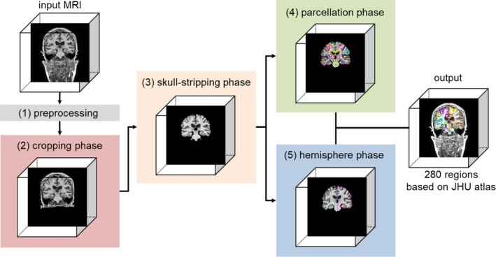
Overview of the open resource for multiple anatomical structure parcellation for T1‐weighted brain MRIs (OpenMAP‐T1) consisting of the preprocessing, cropping phase, skull‐stripping phase, parcellation phase, and hemisphere phase.

2.3.1. Preprocessing

N4 bias field correction (Tustison et al. 2010) was applied to remove intensity nonuniformity. In addition, the images were rescaled to a resolution of 1 × 1 × 1 mm using trilinear interpolation, and their size was standardized to 256 × 256 × 256 through the application of zero padding. Pixels with intensity values below 0 or above u + 2σ (where u is the mean and σ is the standard deviation) were identified as outliers and excluded. These pixels were then linearly normalized to a range between −1 and 1. Following normalization, the excluded pixels were replaced with the minimum and maximum values within this normalized range.

2.3.2. Cropping Phase

Nonbrain soft tissue, such as skin, fat, and muscle, potentially confound whole‐brain parcellation. In particular, variations in the intensity of the neck tissue interferes with image segmentation. In addition, the extent to which the field‐of‐view of the image covers the neck depends on the scan parameters, and, in some publicly available datasets (e.g., NFBS and OASIS1), a defacing algorithm was applied to the image for deidentification (Puccio et al. 2016; Marcus et al. 2007). To reduce the influence of neck tissue in image segmentation and parcellation, we set the cropping phase to eliminate the regions below the brain in a consistent way using the cropping network (CNet). Supporting information: Figure B shows an overview of the cropping phase and the detail of the CNet is shown in Section 2.3.6.

In the training of the CNet, the head region included in the parcellation map resulting from MALF was used (Supporting information: Figure A), since the parcellation map covers the head above the foramen magnum, and does not include neck tissue below it. The CNet employed 2D segmentation on individual cross‐sections of a 3D brain MRI, which were then vertically stacked for high‐speed processing. By utilizing the 2D U‐Net architecture, it was possible to train the model using numerous images from a single MRI. For example, with a 256 × 256 × 256 matrix, 2D U‐Net can utilize 256 slices from a single MRI. Note that the cropping phase was specifically designed to eliminate tissue located below the brain; hence, the axial section, which does not contain vertical information, was excluded from the ensemble. The output was a probability map for the head above the foramen magnum, and areas with a probability of 50% or higher were defined as head masks. A failure in the cropping phase considerably affects the processing performance of subsequent phases. To prevent small gaps or missing areas in the output mask, a closing process was applied using a 3 × 3 × 3 filter. The dilation and erosion operations were performed three times each.

2.3.3. Skull‐Stripping Phase

To further remove signals from extracranial soft tissues that remained after the initial cropping phase, we applied skull‐stripping to the image. Given the varying intensity ranges caused by different scanner types, scan sequences, and parameters, it is essential to adjust the image contrast between gray and white matter, as well as cerebrospinal fluid. However, signals from extracranial soft tissues, such as fat, bone, and muscle, vary greatly and can disrupt the stable signal intensity profile of intracranial structures. This variation can adversely affect the performance of deep‐learning models. By employing skull‐stripping with SSNet, we effectively removed irrelevant regions for the later stages of parcellation and hemisphere analysis. Supporting information: Figure C provides an overview of the skull‐stripping phase and the detail of the SSNet is Section 2.3.6.

To develop SSNet, we trained the model using an intracranial mask obtained from MALF (Supporting information: Figure A). SSNet performs 2D segmentation on any cross‐sectional view of a 3D brain MRI, stacking these sections vertically in a manner similar to that of CNet. We input three cross‐sectional views—sagittal, coronal, and axial—into a 2D‐U‐Net. The output was a label for the intracranial space, defined as an area with a probability of 50% or higher.

2.3.4. Parcellation Phase

In our current computing environment, training a full‐size deep‐learning network for multi‐class parcellation with 3D images, such as an entire brain, presented challenges. To optimize parcellation performance without running graphics processing units (GPU) memory, we used two strategies: utilizing 2D slices, and merging the left and right brain regions. An overview of the parcellation phase can be seen in Supporting information: Figure D.

The PNet, designed for 2D segmentation of 3D brain MRI cross‐sections, stacks these sections vertically. It is important to note that the PNet functions as a 2.5D U‐Net, incorporating a target slice and the slices directly above and below it, and combining these slices along the channel direction. In typical 2D U‐Net applications for 3D images, vertical spatial information is lost. However, the 2.5D U‐Net approach allows for the use of pseudo spatial information while reducing parameter count compared with a 3D U‐Net. Consequently, for each cross‐section, three image slices (256 × 256) are stacked in the depth direction, resulting in an input dimension of 256 × 256 × 3 for the PNet. The choice to stack three slices was based on the findings from preliminary experiments. Furthermore, of the 280 brain regions, those present in both hemispheres were merged as a single region (Supporting information: Figure A). Excluding the 3^rd and 4^th ventricles, 278 regions exist in both the left and right hemispheres, as per the JHU‐MNI atlas. During the parcellation phase, this merging reduces the target regions for PNet to 141, making the segmentation task effectively 142 classes, including the background.

Combining the left and right regions offers three benefits. First, it enables U‐Net to train on larger regions, which is crucial as some of the 280 regions are smaller than 100 voxels and challenging to extract accurately. Merging hemispheres roughly doubles the volume of these regions, making them more tractable. Second, it reduces computational costs. In 2D or 2.5D U‐Net, the dimension of the output parcellation map is height × width × channels (number of segmentation classes). By merging hemispheres, we halve the number of output channels. Third, it facilitates the use of sagittal sections. Normally, distinguishing left from right in sagittal sections is difficult, and can potentially degrade parcellation performance. This issue is resolved by treating the hemispheres as identical.

Unlike CNet and SSNet, PNet uses three models for each cross‐section (coronal, sagittal, axial), and the final prediction is based on the highest average prediction probability across these models. This approach was chosen to ensure consistent predictions in regions where parcellation is challenging, such as at the brain's edges. Training a single model with three cross‐sections risks misidentifications, like mistaking a coronal for an axial section.

2.3.5. Hemisphere Phase

The segmentation task of HNet is a three‐class classification: background; right hemisphere; and left hemisphere. This classification aims to determine the left and right borders of 139 of the 141 region labels generated in the parcellation phase. The hemisphere phase model was trained using hemisphere labels obtained from MALF. An overview of this phase is depicted in Supporting information: Figure E and the detail of the HNet is shown in Section 2.3.6.

HNet employs 2D segmentation on any cross‐section, stacking these sections vertically. It specifically uses axial and coronal sections to output the hemisphere labels. A post‐processing step involving dilation was implemented to separate each region generated during the parcellation phase to the right and left sides. The process is as follows: (1) Dilate only the left hemisphere label. (2) Modify the overlapping parts of the dilated left hemisphere label with the right hemisphere label to be classified as the right side. (3) Dilate only the right hemisphere label. (4) Modify the overlapping parts of the dilated right hemisphere label with the left hemisphere label to be classified as the left side. This method allows the hemisphere labels to expand while minimally affecting the borders.

Finally, the parcellation map, which includes 280 region labels, was created by dividing the 141‐region parcellation map into left and right hemispheres, using the hemisphere labels obtained from the hemisphere phase. It is important to note that, in the 141‐region parcellation map, the two regions without a left–right distinction (3^rd and 4^th ventricles) were given priority over the hemisphere labels (i.e., the hemisphere label was ignored). Furthermore, if there was an overlap between the background from the parcellation phase and the hemisphere region from the hemisphere phase, the background was given precedence.

2.3.6. Structures of CNet, SSNet, PNet, and HNet and Their Training

The CNet, SSNet, PNet, and HNet each comprise 24 convolution layers based on 2D CNN (Figure 2). The main distinction between them lies in the number of input and output channels. As detailed in Figure 2, CNet, SSNet, and HNet had one input channel, while PNet had three channels.

FIGURE 2.

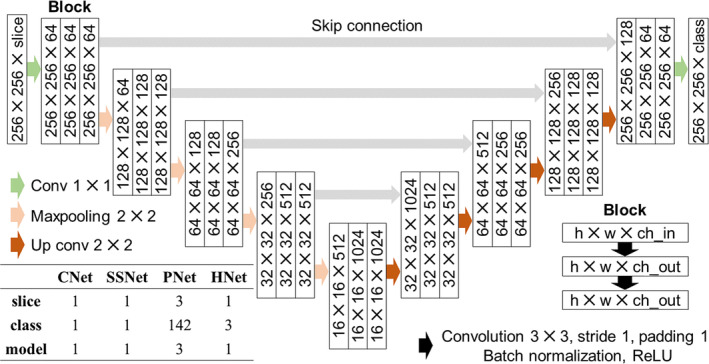
Architecture of the U‐Net (CNet, SSNet, PNet, and HNet). U‐Net consists of nine blocks, and each block includes two convolutions, batch normalization, and a ReLU function. The CNet, SSNet, and HNet have one input channel, and only PNet has three channels, including the target slice and its upper and lower slices. Since the CNet and SSNet perform binary cross entropy, the output class is only one. Also, since the PNet and HNet use multi‐class classification, the output is the number of regions plus one (background). Note that only PNet has three models (for coronal, sagittal, and axial sections).

Data augmentation included a random rotation ranging from −20° to +20° and a random shift from −20 to +20 pixels, applied with an 80% probability. For the sagittal cross‐sections, a broader random rotation range of −30° to +30° was used, based on the greater variation seen on existing MRI databases. To ensure robust performance for low signal‐to‐noise ratio (SNR) images, random Gaussian noise (mean 0, standard deviation 0.25) was added with a 50% probability. These data augmentation techniques were applied consistently across all phases. MRI magnetic field inhomogeneity led to very low‐frequency intensity variations throughout the image. Consequently, a random bias field (Sudre, Cardoso, and Ourselin 2017) was introduced with a 50% probability during the cropping and skull‐stripping phases. While N4 bias field correction was used in preprocessing to address inhomogeneity as much as possible, this data augmentation was implemented to enhance the model's robustness. To adapt the CNet for use with images that did not include the neck area below the foramen magna, commonly found in axial scans and defaced images, we augmented the training data by incorporating images with the neck area cropped out, at a probability of 20%. Similar to CNet, the training dataset for SSNet was augmented by including skull‐stripped images as inputs with a 20% probability. This approach enabled the model to more accurately identify the location of the brain by reducing the impact of non‐brain regions.

The CNet, SSNet, PNet, and HNet were mainly trained using two RTX 3090 GPU with 24GB memory for about 24 h. Also, Automatic Mixed Precision (AMP) was utilized to accelerate training. The number of epochs was set to 10,000, and the learning rate was set to decrease sequentially from 0.01 to 0.0001 by the Cosine Annealing Learning Rate Scheduler. The batch size was 64 on CNet, SSNet, and HNet, and 32 on PNet. For the loss functions, the CNet and SSNet used binary cross‐entropy, while the PNet used a combination of cross‐entropy and Dice loss. The HNet exclusively used cross‐entropy.

2.4. Evaluation and Comparison of Parcellation Performance

We assessed the performance of OpenMAP‐T1 in terms of agreement with the GT manual labels, and in comparison to MALF, FreeSurfer, biological criteria, and processing time.

2.4.1. Agreement With GT Manual Labels

2.4.1.1. Parcellation Performance

To evaluate the parcellation performance of OpenMAP‐T1, two metrics were used: (1) an illustration of the spatial overlap between two parcellation maps generated by manual labels and OpenMAP‐T1 derived by calculating the average Dice similarity coefficient (DSC); (2) a demonstration of the average 95th percentile Hausdorff distance (HD) between manual labels and OpenMAP‐T1, which showed the quality of parcellation boundaries. DSC and HD metrics were calculated for cortical (ROI = 74), deep gray matter (ROI = 26), white matter (ROI = 116), and others (ROI = 64).

To assess the performance of the multi‐phase U‐Net model introduced in OpenMAP‐T1, we compared its ability to parcellate the brain with a patch‐based 3D U‐Net introduced in nnUNet (Isensee et al. 2021). We chose the nnUNet as a comparison target since it is a commonly used tool for segmenting medical images and has been proven to demonstrate excellent performance. Direct comparison with existing deep‐learning‐based parcellation tools such as SLANT (Huo et al. 2019) and FastSurfer (Henschel et al. 2020) was not possible because they use different anatomical definitions compared to OpenMAP‐T1, which follows the JHU‐MNI atlas definition. Both nnUNet and OpenMAP‐T1 were trained on the same MRI images (350 cases in ADNI2) to parcellate the brain into 280 anatomical regions. We used an analysis of variance (ANOVA) for this comparative analysis. A p value less than 0.05 in two‐sided tests was considered statistically significant.

2.4.1.2. Influence of Biological and Pathological Factors

To apply the parcellation methods in large‐scale clinical research, they must be robust to differences in age, sex, and diagnosis. We conducted a comparative analysis to determine whether significant variations in the DSC were present due to biological factors such as age, sex, and diagnosis. We used an ANOVA for this analysis and considered a p value less than 0.05, corrected for multiple comparisons using the Bonferroni method, in two‐sided tests, as statistically significant.

2.4.1.3. Volumetric Similarity

To investigate whether the regional volumes obtained from OpenMAP‐T1 corresponded to the GT, three metrics were used:

1. Pearson and Spearman correlation coefficients were calculated to measure the correlation between volumes obtained from GT manual labels and OpenMAP‐T1, indicating the consistency of the relationship between these predicted volumes.

2. A Bland–Altman plot (Altman and Bland 2018) to examine the agreement between regional volumes obtained from manual labels and OpenMAP‐T1, which allowed the identification of any systematic bias between the measurements and outliers.

3. The correlation between the volume obtained from manual labels and the corresponding DSC was analyzed to show how the volume correlated with parcellation performance.

All these metrics were calculated for cortical (ROI = 74), deep gray matter (ROI = 26), white matter (ROI = 116), and others (ROI = 64).

2.4.2. Comparison With MALF

Our aim was to create a fast model that could accurately parcellate the whole brain, similar to MALF. To achieve this, we evaluated the agreement between the ROIs obtained from OpenMAP‐T1 and that of MALF.

2.4.2.1. Parcellation Similarity

An average DSC was used as a measure to evaluate the spatial overlap between ROIs obtained from MALF and OpenMAP‐T1. DSC was calculated for cortical (ROI = 74), deep gray matter (ROI = 26), white matter (ROI = 116), and others (ROI = 64).

2.4.2.2. Influence of Technical, Biological, and Pathological Factors

We conducted an ANOVA to analyze how age, sex, scanner manufacturer, and field strength affected the agreement between MALF and OpenMAP‐T1. We investigated whether these factors affected the DSC. A p value less than 0.05 in two‐sided tests was considered statistically significant. We did not perform corrections after multiple comparisons, as our aim was to identify factors that could potentially influence the agreements between the two methods.

2.4.2.3. Volumetric Similarity

To determine whether the regional volumes obtained from OpenMAP‐T1 were comparable to those obtained from MALF, three metrics were employed: the correlation between regional volumes; the Bland–Altman plot; and the correlation between volumes obtained from MALF and the corresponding DSC. This comparison was carried out in a manner similar to the comparison with the GT manual labels.

2.4.3. Comparison With FreeSurfer

Various whole‐brain parcellation tools have been developed to date. Among them, FreeSurfer (Version 7.4.1) (Fischl 2012) remains the most commonly used tool. Comparing the ROIs obtained from FreeSurfer and OpenMAP‐T1 is essential to provide valuable insights for prospective users.

It is important to keep in mind that a direct comparison between the parcellation maps of FreeSurfer (based on the Desikan–Killiany–Tourville, DKT) atlas (Klein and Tourville 2012) and OpenMAP‐T1 (which uses the JHU‐MNI atlas Oishi et al. 2009), is not feasible because their anatomical definitions differ.

Therefore, we focused on comparing three regions: the hippocampus; amygdala; and entorhinal cortex. These regions are notably associated with AD. Two metrics were used for this comparison:

1. The average recall, precision, and DSC for the parcellation maps of the hippocampus, amygdala, and entorhinal cortex produced by OpenMAP‐T1 and FreeSurfer, considering the result of FreeSurfer as the GT;

2. A correlation analysis of the volumes for the hippocampus, amygdala, and entorhinal cortex, comparing the results from OpenMAP‐T1 and FreeSurfer.

2.4.4. Biological Evaluation

We assessed the ability to distinguish between AD and cognitively normal (CN) participants using region volumes obtained from FreeSurfer, MALF, or OpenMAP‐T1. Our evaluation involved 554 subjects from the ADNI3 dataset, and we used a three‐fold cross‐validation approach along with a logistic regression model that employed the Least Absolute Shrinkage and Selection Operator (LASSO) for classification.

To ensure a fair comparison with FreeSurfer, we removed volumetric information related to the white matter and the sulcus from MALF and OpenMAP‐T1. In addition, we averaged the predicted volumes of regions obtained from FreeSurfer, MALF, and OpenMAP‐T1 across their left and right counterparts to mitigate multicollinearity, resulting in 58 ROIs for MALF and OpenMAP‐T1 and 59 ROIs for FreeSurfer. In addition, we adjusted for brain size effects by normalizing each structure's volume to the total brain volume of each participant. These normalized volumes were then transformed into z‐scores, based on the mean and standard deviation, and used as input variables for the model. The classification performance was compared using the area under the curve (AUC) from receiver operating characteristic (ROC) curve analysis, with significant differences determined using DeLong's algorithm (Sun and Xu 2014). A p value less than 0.05 in two‐sided tests was considered statistically significant. We used the coefficients of the LASSO model to identify the top 20 anatomical areas crucial in the classification.

3. Results

3.1. Agreement With GT Manual Labels

3.1.1. Parcellation Performance

Table 3 and Figure 3 compare the parcellation results of 3D U‐Net (nnUNet) and OpenMAP‐T1 when the manual labels of JHU multi‐atlas library were set to GT. In DSC, OpenMAP‐T1 significantly outperformed 3D U‐Net in the 8–19 age range for cortical and white matter, and in HD, OpenMAP‐T1 significantly outperformed 3D U‐Net except in the 50–90 age range for deep gray matter. In addition, there were multiple outliers in DSC for 3D U‐Net compared to OpenMAP‐T1.

TABLE 3.

Comparison of 3D U‐Net (nnUNet) and OpenMAP‐T1 in Dice similarity coefficient (DSC) and 95th percentile Hausdorff distance (HD) for cortical (ROI = 74), deep gray matter (ROI = 26), white matter (ROI = 116), and others (ROI = 64).

	Age	Method	DSC	HD		DSC	HD
Cortical (ROI = 74)	8–19	3D U‐Net (nnUNet)	0.689 (±0.080)	13.8 (±10.1)	Deep gray matter (ROI = 26)	0.803 (±0.041)	3.7 (±3.1)
		OpenMAP‐T1	0.740 (±0.027)	3.8 (±0.5)		0.817 (±0.027)	1.6 (±0.2)
		ANOVA	p < 0.001	P < 0.001		p = 0.089	p < 0.001
	22–50	3D U‐Net (nnUNet)	0.737 (±0.085)	9.3 (±10.7)		0.845 (±0.034)	2.7 (±3.3)
		OpenMAP‐T1	0.767 (±0.027)	2.9 (±0.3)		0.855 (±0.010)	1.3 (±0.1)
		ANOVA	P = 0.089	p = 0.004		p = 0.145	p = 0.037
	50–90	3D U‐Net (nnUNet)	0.759 (±0.092)	4.8 (±3.7)		0.828 (±0.074)	1.6 (±0.4)
		OpenMAP‐T1	0.794 (±0.033)	2.7 (±0.4)		0.847 (±0.030)	1.4 (±0.2)
		ANOVA	p = 0.094	p = 0.009		p = 0.277	p = 0.051
White matter (116)	8–19	3D U‐Net (nnUNet)	0.684 (±0.078)	11.2 (±7.9)	Others (ROI = 64)	0.620 (±0.066)	10.5 (±6.4)
		OpenMAP‐T1	0.727 (±0.027)	3.6 (±0.7)		0.623 (±0.031)	5.2 (±0.7)
		ANOVA	p = 0.002	P < 0.001		P = 0.089	P < 0.001
	22–50	3D U‐Net (nnUNet)	0.736 (±0.075)	8.1 (±8.8)		0.689 (±0.046)	8.6 (±7.0)
		OpenMAP‐T1	0.760 (±0.022)	3.0 (±0.4)		0.701 (±0.032)	4.5 (±0.5)
		ANOVA	p = 0.114	p = 0.005		P = 0.145	P = 0.004
	50–90	3D U‐Net (nnUNet)	0.744 (±0.085)	4.6 (±2.8)		0.717 (±0.092)	5.8 (±2.5)
		OpenMAP‐T1	0.774 (±0.032)	2.9 (±0.5)		0.748 (±0.037)	4.0 (±0.9)
		ANOVA	p = 0.118	p = 0.006		P = 0.277	p = 0.003

Note: Bold type indicates scores where OpenMAP‐T1 significantly outperformed 3D U‐Net (nnUNet).

FIGURE 3.

Boxplots of 3D U‐Net (nnUNet, blue) and OpenMAP‐T1 (orange) in Dice similarity coefficient (DSC) and 95th percentile Hausdorff distance (HD) by age for cortical (ROI = 74), deep gray matter (ROI = 26), white matter (ROI = 116), and others (64). Black stars indicate significant differences between 3D U‐Net (nnUNet) and OpenMAP‐T1. Orange stars indicate significant differences due to age.

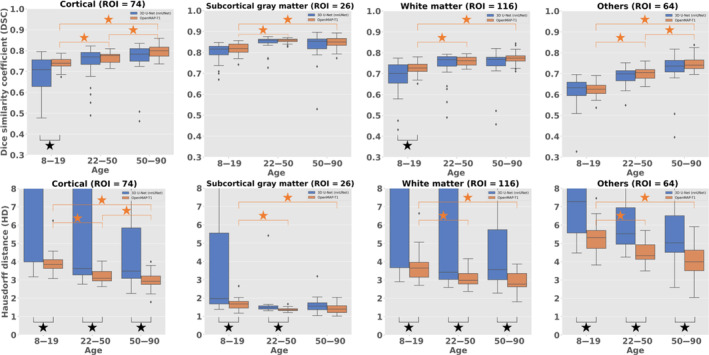
3.1.2. Generalizability

Figures 3 and 4 illustrate the DSC and HD across age, sex, and diagnosis. The DSC value was greater than 0.7 in all conditions. However, age was observed to affect the performance of OpenMAP‐T1 significantly. The DSC tended to be lower in adolescents and young adults than in older adults. Similarly, the HD results also showed that OpenMAP‐T1 performed best for images of older adults. The sex did not affect DSC and HD. The diagnosis significantly affected the DSC and HD values, with decreased performance for individuals with AD compared with the CN group. Please refer to Supporting information: Table B for further details on the ANOVA results of each biological effect.

FIGURE 4.

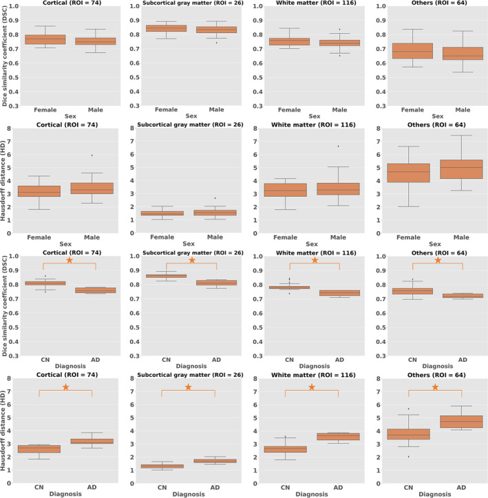
Boxplots of Dice similarity coefficient (DSC) and 95th percentile Hausdorff distance (HD) with biological effects (sex, diagnosis) for cortical (ROI = 74), deep gray matter (ROI = 26), white matter (ROI = 116), and others (64).

3.1.3. Volumetric Analysis

The results of an analysis comparing manual labels to OpenMAP‐T1 for region volumes are presented in Figure 5A. The analysis found a significant correlation with correlation coefficients above 0.95 when using both the Pearson and Spearman methods. Figure 5B, which shows a Bland–Altman plot, demonstrates excellent agreement between the manual labels and OpenMAP‐T1, with most regions having errors within the 2σ range. However, a few regions had disagreements exceeding 2σ. Figure 5C demonstrates a weak correlation between the volumes of the regions and their DSC. Specifically, the correlation was found to be R = 0.138 for cortical, R = 0.649 for deep gray matter, R = 0.379 for white matter, and R = 0.201 for others. This weak correlation implies that smaller regions tend to have greater discrepancies between the measurements from manual labels and OpenMAP‐T1 despite most regions having a DSC higher than 0.7.

FIGURE 5.

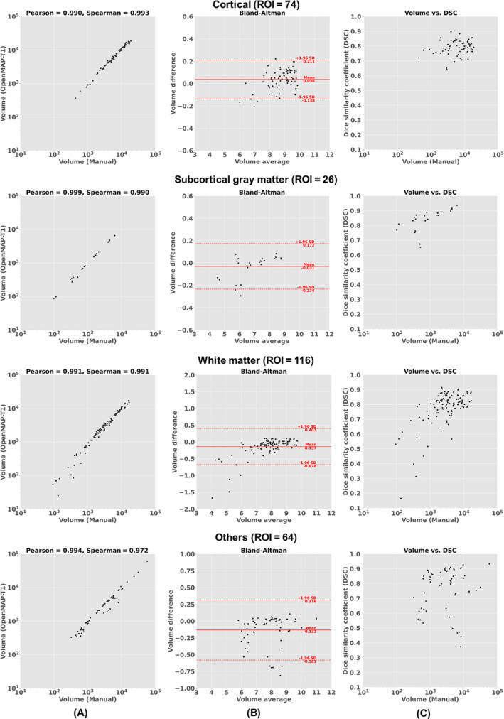
(A) Correlation between the volumes obtained using manual labels and OpenMAP‐T1. (B) Bland–Altman plot demonstrates the relationship between regional volumes obtained from manual labels and a volume difference between manual labels and OpenMAP‐T1. The volume measurements were transformed using a base‐2 logarithmic scale. (C) Relationship between the structural volume obtained from manual labels and the Dice similarity coefficient (DSC) between manual labels and OpenMAP‐T1.

3.2. Comparison With MALF

3.2.1. Parcellation Performance

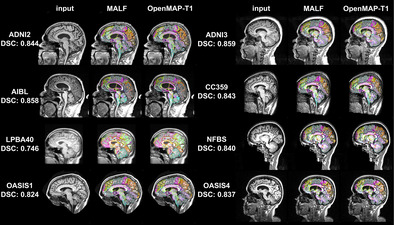
Figure 6 shows a comparative analysis of parcellation results between MALF and OpenMAP‐T1. Despite significant variations in head appearance across different datasets, OpenMAP‐T1 demonstrated satisfactory performance for all eight datasets. Notably, the median DSC exceeded 0.8 for every dataset, with the exception of LPBA40, which did not utilize MPRAGE imaging.

FIGURE 6.

Representative results from MALF and OpenMAP‐T1 are demonstrated. The median Dice similarity coefficient (DSC) calculated between the two sets of results is provided. Note that defacing techniques have been implemented on NFBS and OASIS1 datasets to safeguard the privacy of the participants.

Figure 7 shows the average DSC obtained from comparing 280 anatomical regions in the parcellation maps between MALF and OpenMAP‐T1. These scores, exceeding 0.75 in all datasets, signified a considerable level of agreement between the two methods. However, it should be noted that some datasets displayed extreme outliers.

FIGURE 7.

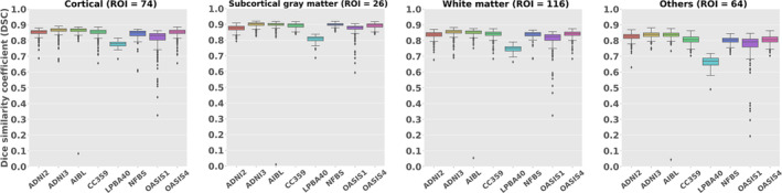
Boxplots of the Dice similarity coefficient (DSC) for cortical (ROI = 74), deep gray matter (ROI = 26), white matter (ROI = 116), and othres (64) across each dataset.

Figure 8 shows the image with the lowest average DSC of 280 anatomical regions and its underlying causes. The causes were predominantly attributed to mislabeling by MALF, except for one image from OASIS4. In the image from ADNI2, ROIs for gray and white matter in the cerebellum erroneously included neck areas. In the image from ADNI3, a portion of the occipital lobe was absent from the parcellation map. The image from AIBL was affected by extremely high‐intensity noise, leading to significant mislabeling in the MALF results. In the image from CC359, the labels extended beyond the parietal lobe boundaries. In images from LPBA40 and OASIS1, parts of the cerebellum were missing in the parcellation map, a pattern also observed in other OASIS1 images. The image from NFBS had an issue with a missing section of the frontal lobe in its parcellation map. The exception was an image from OASIS4 with a large arachnoidal cyst that neither method successfully labeled.

FIGURE 8.

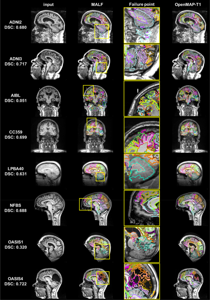
Image with the lowest average Dice similarity coefficient (DSC) from all datasets (From left to right: Input image, output of MALF, enlarged image of MALF failure point, output of OpenMAP‐T1). The yellow squares on the images in the second column correspond to the enlarged images in the third row and highlight areas where the MALF's parcellation failed.

3.2.2. Influence of Biological and Technical Effects

Figure 9 shows the DSC across biological (age, sex, and diagnosis) and technological (scanner manufacturer and field strength) categories, for the ADNI3 and OASIS4 datasets. The results from other databases are provided Supporting information: Table C. The red boxplots illustrate the influence of biological factors, while the blue boxplots represent the impact of technological factors. The DSC exceeded 0.8 in all conditions. Age had a significant effect in ADNI2, where the DSC tended to decrease in individuals in their 90s. A similar trend was observed in OASIS4, although the effect was not statistically significant. No significant differences were noted based on sex in either database. Regarding the diagnosis, a significant effect was observed in OASIS4, where a diagnosis of VCI was associated with lower DSC compared to other diagnoses (Supporting information: Table D); however, in ADNI3, the diagnosis did not significantly affect DSC. Among the scanner manufacturers, GE systems showed lower DSC compared with those from Philips and Siemens. In terms of field strength, scanners operating at 1.5T had a lower DSC compared with those operating at 3T.

FIGURE 9.

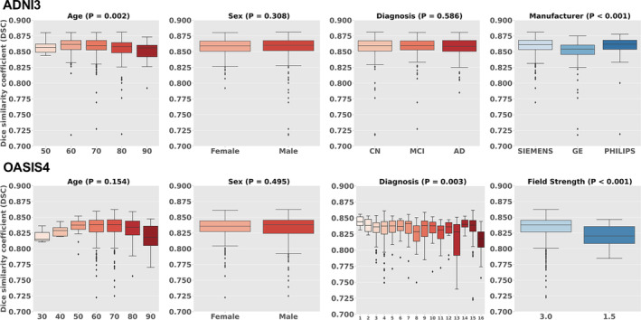
Boxplots of biological (age, sex, diagnosis) and technological effects (manufacturer and field strength) with Dice similarity coefficient (DSC). OASIS4 includes 16 diagnostic labels: 1: AD variant; 2: AD + non neurodegenerative; 3: AD/vascular; 4: Alzheimer disease dementia; 5: Cognitively Normal (CN); 6: Dementia with Lewy Bodies (DLB); 7: early onset AD; 8: Frontotemporal Dementia (FTD); 9: Mild Cognitive Impairment (MCI); 10: mood/polypharmacy/sleep; 11: non‐neurodegenerative neurologic disease; 12: other‐miscellaneous; 13: other non‐AD neurodegenerative disorder; 14: primary progressive aphasia (PPA); 15: uncertain—AD possible; 16: Vascular Cognitive Impairment (VCI).

3.2.3. Volumetric Similarity

Figure 10A shows a comparison of the region volumes predicted by MALF and OpenMAP‐T1 for the ADNI3 and OASIS4 databases. The correlation coefficients for these comparisons were above 0.99 using both the Pearson and Spearman methods, indicating an almost perfect correlation. The Bland–Altman plot of Figure 10B revealed that the majority of regions had errors within the 2σ range, demonstrating excellent agreement between MALF and OpenMAP‐T1. However, a few regions in both the ADNI3 and OASIS4 databases exhibited disagreements exceeding 2σ. Figure 10C shows a weak correlation between the volumes of the regions and their DSC (R = 0.660 in ADNI3, R = 0.707 in OASIS4), despite most regions having a DSC higher than 0.7. This implies that smaller regions tend to have greater discrepancies between the measurements from MALF and OpenMAP‐T1. Additional results for other databases can be found Supporting information: Figures F–H.

FIGURE 10.

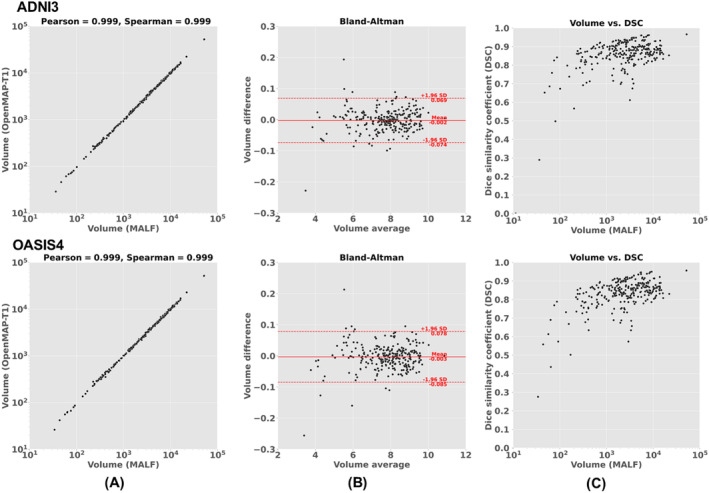
(A) Correlation between the predicted volumes obtained using MALF and OpenMAP‐T1. (B) Bland–Altman plot to demonstrate agreement between regional volumes predicted by MALF and OpenMAP‐T1. The volume measurements were transformed using a base‐2 logarithmic scale. (C) Relationship between the structural volume obtained from MALF and the Dice similarity coefficient (DSC) between MALF and OpenMAP‐T1.

We noted that certain anatomical labels were absent from the predicted parcellation map produced by OpenMAP‐T1, specifically in the right rostral anterior cingulate white matter and the bilateral fimbria. A similar trend of omitting these small structures was observed with MALF. MALF results were as follows: 1.26 mm³ with 924 of 929 instances for the right rostral anterior cingulate white matter; 6.37 mm³ with 493 of 929 instances for the left fimbria; and 12.86 mm³ with 136 of 929 instances for the right fimbria.

3.3. Comparison With FreeSurfer

Figure 11 shows the recall, precision, and DSC for the hippocampus, amygdala, and entorhinal cortex in the parcellation maps of OpenMAP‐T1 and FreeSurfer, considering the results of FreeSurfer as the GT. Figure 12 compares the volumes in the hippocampus, amygdala, and entorhinal cortex between OpenMAP‐T1 and FreeSurfer. In the hippocampus, the recall, precision, and DSC were all high. This result indicated that the definition of the hippocampus boundary was nearly identical in OpenMAP‐T1 and FreeSurfer, and both methods were equally accurate in identifying the hippocampus. As shown in Figure 12, the hippocampal volume measurements obtained by both methods correlated well. In the amygdala, although the recall was equivalent to that of the hippocampus, the precision and DSC were lower. This suggests the existence of a systematic bias due to methodological differences in defining the amygdala region; the amygdala region defined by FreeSurfer was smaller than that defined by OpenMAP‐T1, which included the cortical amygdala not included in the FreeSurfer definition. As demonstrated in Figure 12, although the volume measurements of both methods correlated well, FreeSurfer consistently underestimated the amygdala volume compared with OpenMAP‐T1. Conversely, FreeSurfer defined the entorhinal cortex area as larger than OpenMAP‐T1 and often included the adjacent dura mater within the entorhinal cortex region (see Figure 13). Therefore, while precision was relatively preserved, the recall and DSC were lower, and the correlation of volume measurements between the two methods was weaker for the entorhinal cortex compared with the hippocampus and amygdala.

FIGURE 11.

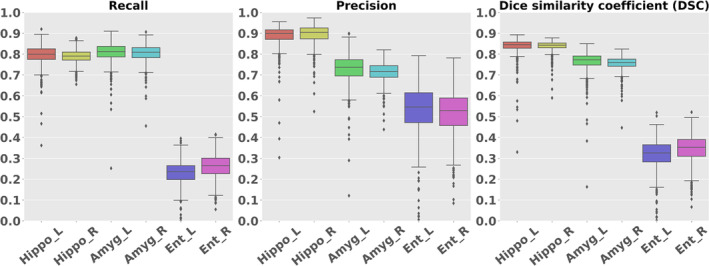
Boxplot of the Recall, Precision, and Dice similarity coefficient (DSC) in the hippocampus, amygdala, and entorhinal regions.

FIGURE 12.

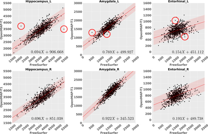
The correlations between the predicted volumes of the hippocampus, amygdala, and entorhinal cortex as obtained by OpenMAP‐T1 and FreeSurfer. The upper row displays the results from the left side, while the lower row presents the results from the right side in ADNI3. The red lines represent the regression lines, while the transparent red areas show the range encompassing three standard deviations from these fitted regression lines. In the right‐bottom corner, the equation of the regression line is provided, where X represents the volume acquired by FreeSurfer. The red circles in the graph correspond to the representative images showcased in Figure 13.

FIGURE 13.

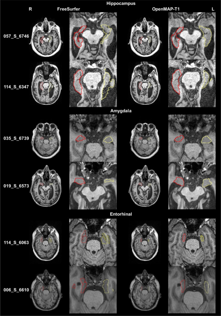
The parcellation maps from OpenMAP‐T1 and FreeSurfer overlaid on the MPRAGE images that correspond to the red circles in Figure 12 are demonstrated. The leftmost column shows the study IDs from the ADNI3 dataset. Axial slices along with magnified images of the hippocampus, amygdala, and entorhinal cortex are presented. The red borderlines indicate the regions on the right side, while the yellow borderlines mark the regions on the left side. These images adhere to the radiological convention, where the left side of the brain is shown on the right side of the image.

Figure 13 displays representative images linked to the outliers in Figure 12. The primary reasons for the low DSC were generally due to mislabeling by FreeSurfer, differences in anatomical definitions between OpenMAP‐T1 and FreeSurfer, or a combination of both. For instance, in image 057_S_6746, FreeSurfer incorrectly labeled the left hippocampus. In image 114_S_6347, FreeSurfer erroneously included a part of the lateral ventricle in the left hippocampus ROI. The boundary of the amygdala was delineated smaller by FreeSurfer than defined by OpenMAP‐T1 in images 035_S_6739 and 019_S_6573, which was attributable to the differing anatomical definitions between the two. Furthermore, FreeSurfer typically incorporated the perirhinal cortex and the dura mater adjacent to the entorhinal cortex into the entorhinal ROI. In contrast, the definition of the entorhinal cortex in OpenMAP‐T1 did not include these areas, as evident in images 114_S_6063 and 006_S_6610.

3.4. Biological Evaluation

AUC values for the ROC curves (Figure 14) were 0.916 for MALF, 0.912 for OpenMAP‐T1, and 0.916 for FreeSurfer. There were no significant differences between these AUC values. The p values derived from the DeLong test were 0.666 when comparing MALF and OpenMAP‐T1, and 0.493 when comparing OpenMAP‐T1 and FreeSurfer.

FIGURE 14.

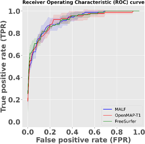
The receiver operating characteristic (ROC) curve to distinguish between Alzheimer's disease (AD) and cognitively normal (CN) based on predicted volumes using the LASSO model. The blue line represents the ROC curve for MALF, the red line for OpenMAP‐T1, and the green line for FreeSurfer. The shaded areas around each line indicate the standard deviation.

Among the top 20 anatomical regions with the highest correlation coefficients derived from the trained LASSO model, 11 structures were common between MALF and OpenMAP‐T1 (Figure 15). Of these, six structures—namely the hippocampus, amygdala, inferior horn and body of the lateral ventricle, and the parahippocampal gyrus—are known to be associated with AD pathologies (Chupin et al. 2009; Uchikado et al. 2006; Thompson et al. 2004, 1998), indicating the appropriateness of the LASSO model.

FIGURE 15.

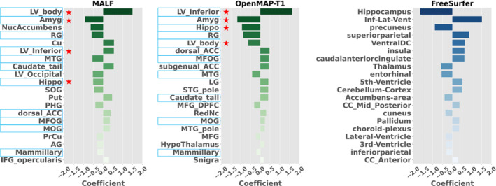
The 20 anatomical regions that exhibited the highest correlation coefficients, as determined by the trained LASSO model. Light blue highlights common regions between MALF and OpenMAP‐T1. Red stars show regions associated with Alzheimer's disease (AD).

3.5. Runtime

OpenMAP‐T1 performed complete parcellation at 90 s/case using a single GPU (RTX3090) and 10 min/case using a CPU (i9‐10980XE). This result shows that OpenMAP‐T1 is 40 times faster than MRICloud, which is 1 h/case.

4. Discussion

We have developed and released a deep‐learning model, OpenMAP‐T1, on GitHub to segment and parcellate brain 3D T1‐weighted MRI images based on their anatomical structures. The performance of the model was evaluated using metrics such as DSC and HD, and was correlated based on comparisons between the OpenMAP‐T1 and the manual labels. The results show that the parcellation outcomes of OpenMAP‐T1 were superior to the baseline (3D U‐Net) and substantially agreed with the existing MALF method. Notably, the processing time was significantly reduced to less than 90 s per image, compared to the several hours required by the existing MALF method.

There is the potential to further enhance the processing speed of OpenMAP‐T1. For instance, reducing the image matrix size could decrease the input size for the PNet. This reduction can be achieved by repositioning the center of gravity of the brain post skull‐stripping, and then trimming areas outside the brain. We anticipate periodic updates to OpenMAP‐T1, focusing on optimizing processing strategies and incorporating new features into the algorithms.

4.1. Evaluation With GT Manual Labels

The multi‐phase U‐Net structure adopted for OpenMAP‐T1 significantly outperformed the 3D U‐Net implemented in nnUNet. Notably, OpenMAP‐T1 had fewer outliers with low DSC than 3D U‐Net. This result shows that the multi‐phase strategy introduced in OpenMAP‐T1 constructs a robust model for various imaging environments, compared to a single‐phase 3D U‐Net model that directly generates a parcellation map. In the parcellation phase of the OpenMAP‐T1, the whole brain was parcellated into 141 regions, combining left and right labels. This approach was inspired by the approach used in FastSurfer (Henschel et al. 2020), which reduced the number of classes (i.e., region labels) and increased each region's size, resulting in accurate parcellation.

The OpenMAP‐T1 demonstrated the best performance in images of individuals aged between 50 and 90 years of age. However, it was also applicable for images of individuals between 22 and 50 years of age, with the mean DSC exceeding 0.7 in both age groups. In contrast, the mean DSC was found to be below 0.7 in certain regions for individuals between 8 and 19 years of age. This reduction in DSC may be attributed to the age range of the training data, which was between 55 and 95 years of age. To improve the model performance, MRIs from younger age groups could be included to train the OpenMAP‐T1. Furthermore, the parcellation performance of OpenMAP‐T1 was not affected by sex and only slightly decreased in cases of AD. With a DSC above 0.7 for cortical, deep gray matter, and white matter, the performance of this algorithm is considered in substantial agreement with the GT.

The volume of each region of the parcellation map obtained from OpenMAP‐T1 was strongly correlated with that obtained from manual labels. However, the DSC tends to be lower for small regions than for regions with larger volumes. Notably, DSC was lower in sulci with significant individual differences in their volumes.

4.2. Comparison With MALF

The performance of the OpenMAP‐T1 was mostly equivalent to MALF, while the processing speed was significantly faster than MALF. There were some images in which OpenMAP‐T1 and MALF showed disagreement. For these cases, MALF tended to mislabel images with noticeable intensity inhomogeneity even after correction with the N4 algorithm. For instance, MALF tended to mislabel images scanned with 3D‐SPGR sequences on 1.5T scanners (LPBA40), with lower contrasts between the white matter and gray matter than MPRAGE on 3T scanners. MALF also tended to mislabel images that had undergone defacing (NFBS and OASIS1). Therefore, the low DSC was due to mislabeling in MALF rather than OpenMAP‐T1.

MALF uses whole‐head MPRAGE images scanned on 3T scanners as training data and employs image transformation using intensity information as a cost function (Mori et al. 2016). Therefore, MALF is vulnerable to intensity inhomogeneity, and its parcellation accuracy might be affected by differences in scanner magnetic field strength, scan protocols, and defacing. In contrast, OpenMAP‐T1, which uses deep‐learning with data augmentation, was more robust than MALF against variations in image intensity inhomogeneity and scanning parameters.

Images with notable intensity inhomogeneity, even after intensity correction, were often scanned in a head‐extended position (ADNI2 and ADNI3 in Figure 8). Such a position is often seen in older participants with neurological conditions (Kashihara and Imamura 2013; Muller et al. 2002), leading to a decrease in image intensity in areas distant from the physical center of the MRI scanner, such as the frontal pole or the posteroinferior occipital lobe and cerebellum. The robustness of OpenMAP‐T1 for the abnormal head position seems advantageous for the analysis of disease images. Moreover, artifacts that introduce high‐signal pixels potentially hinder successful intensity correction (AIBL in Figure 8). The results with OpenMAP‐T1 indicated its robustness against such artifacts.

It has been demonstrated that facial appearance can be reconstructed from a whole‐head MRI (Schwarz et al. 2021). Therefore, defacing may become a standard procedure when sharing brain MRI images (Weiner et al. 2023; Theyers et al. 2021; Rubbert et al. 2022). However, many brain parcellation methods have not been tested on images that have undergone defacing. Implementing a refacing process, which adds artificial facial information after defacing, is being considered to avoid changes in parcellation accuracy due to defacing (Schwarz et al. 2021). The ability of automated brain parcellation methods to handle such defaced MRIs is crucial in the era of open science and data sharing. Meanwhile, OpenMAP‐T1 has demonstrated its capability to parcellate images from the NFBS and OASIS1 databases, which have used different defacing methods, indicating its adaptability for future mainstream databases of defaced images.

In recent years, the MPRAGE sequence with 3T scanners has been often used for anatomical MRI scans for brain research (Ai et al. 2021). However, available open brain MRI databases contain legacy images scanned with MRI scanners from various vendors, models, and magnetic field strengths. These databases also include images scanned with the MPRAGE and other sequences, such as the SPGR sequence. The accuracy of brain parcellation was affected by variations in scanner types, magnetic field strengths, and scan protocols (Figure 9) (Arai et al. 2021; Zuo et al. 2023). Thus, automated brain MRI parcellation methods should be robust to these variations. Our results showed that the parcellation maps generated by MALF and OpenMAP‐T1 are substantially similar (average DSC > 0.8, except for LBPA40 database that collected SPGR images) regardless of the scanner vendor, magnetic field strength, scan protocol, or the presence of defacing. However, we found that DSC were significantly lower in SPGR images than those in MPRAGE images, from 1.5T to 3T scanners, as well as the DSC in GE scanners, which were significantly lower compared with those in Philips or Siemens.

From the perspective of precision medicine, a significant topic has been whether insights gained from basic research and clinical trials can be adapted to actual clinical data. Research often involves strict inclusion and exclusion criteria, targeting specific individuals, inevitably leading to selection bias (Jaramillo et al. 2007; LeWinn et al. 2017; Cavallari et al. 2022). Therefore, using real‐world data is essential when considering the applicability to clinical data. To develop automated brain MRI parcellation methods, it is crucial to assess their accuracy using brain images obtained through clinical practice. To evaluate the applicability of OpenMAP‐T1 in real clinical settings, we used real‐world data from OASIS4. The average DSC exceeded 0.8 in OASIS4, suggesting potential adaptability to images obtained through clinical practice.

When testing research data such as ADNI, the DSC was unaffected by sex or diagnostic category, including CN, MCI, and AD. However, in the real‐world data of OASIS4, while the DSC was not influenced by age or sex, it was affected by clinical diagnosis. Average DSC of groups with “other non‐AD neurodegenerative disorders” and “vascular cognitive impairment” tended to be lower than other diagnostic groups, although they still demonstrated average DSC above 0.8. Many images with DSC below 0.8 were due to mislabeling by MALF in the presence of lesions, but, in patients with large arachnoid cysts at the posterior area, both MALF and OpenMAP‐T1 mislabeled the lesion. This result suggests that OpenMAP‐T1 may mislabel images containing large lesions, likely due to a lack of such images in its training data, indicating potential areas for future improvement.

The volumes of regions obtained from OpenMAP‐T1 and MALF were similar and well correlated, demonstrating that the volumetric result of OpenMAP‐T1 is almost identical to MALF, even for small regions. Based on their volumetric results, there was no difference in the ability to classify AD and CN between MALF and OpenMAP‐T1. The important regions for the AD‐CN classification derived from the OpenMAP‐T1‐based and MALF‐based classification models highly overlapped between the two models. This result shows that OpenMAP‐T1 can be an alternative method applicable to neuroscience research that aims to extract clinically relevant information from volumetric results.

4.3. Comparison With FreeSurfer

FreeSurfer (Fischl 2012) is one of the most commonly used software packages for brain MRI parcellation (Arslan et al. 2018; Eickhoff, Yeo, and Genon 2018). FreeSurfer is suitable for comprehensive analysis of the cerebral cortex, with its ability to measure the thickness of the cerebral cortex. However, OpenMAP‐T1 can parcellate both gray and white matter areas, thus offering the advantage of simultaneous analysis of the cortex and white matter. Since the definitions of the brain regions employed by both software packages differ, and their intended uses are different, it is difficult to compare the parcellation performance of the two. Therefore, their performance was compared in a task that separated the brain MRIs of AD and CN individuals. In AD research, the amygdala, entorhinal cortex, and hippocampus volumes are often used as neurodegeneration markers. When comparing these volumes measured by FreeSurfer and OpenMAP‐T1, a good correlation was found in these regions. On the other hand, OpenMAP consistently reported larger amygdala volumes than FreeSurfer. This bias does not stem from inaccuracies in delineating structural boundaries. It merely shows a difference in anatomical boundary definition. Namely, the JHU‐MNI Atlas includes the cortical amygdala as part of the amygdala, whereas the DKT Atlas excludes this region from its amygdala definition. What is most important for neuroimaging and clinical applications is the high level of correlation between the two methods; for instance, small structures must be consistently identified as small in both OpenMAP‐1 and FreeSurfer, and large structures as large. This consistency is the critical factor for ensuring reliable measurement and comparability across applications.

The brain regions that played a significant role in separating AD and CN, obtained from the LASSO model, were similar, and there was no difference between FreeSurfer and OpenMAP‐T1 in separation performance for AD and CN, as analyzed by ROC analysis. Therefore, the choice between FreeSurfer and OpenMAP‐T1 should not be based on which has more accurate parcellation, but should be selected according to the research objectives and the anatomical structures of interest.

5. Limitations

OpenMAP‐T1 has several limitations. As with any parcellation method, in small ROIs, precision, recall, and DSC can be significantly reduced by minor boundary differences, making it challenging to evaluate the accuracy of parcellation itself. Furthermore, whether parcellation can be accurately performed on images containing various lesions, such as large cerebral infarcts, brain hemorrhages, or brain tumors, is a topic for future investigation. Using real clinical images as training data for clinical applications might be necessary. Also, while the analyzed images in this study were high‐resolution 3D images, many clinical images use 2D imaging methods with a thickness of 5 mm or more. Whether OpenMAP‐T1 can be applied to such thick‐slice 2D images is also a subject for future study. The current model performed best on images of older adults, likely because we trained the model using images of older adults. We plan to enhance the model by including images of younger individuals to make it more robust across different age groups. This Technical Report aims to demonstrate the effectiveness of the cascading structure that sequentially applies the four U‐Net architectures and provides readers with practical solutions for the fine gray and white matter parcellation. We have deferred the development of a tool to support model training to a later project since generating a model training tool applicable for various types of atlases is still an ongoing area of active research; such tools would need an automated algorithm to fine‐tune hyperparameters specific to each atlas, along with validation studies.

6. Conclusion

We have developed OpenMAP‐T1, a deep‐learning model that can accurately segment and parcellate brain T1‐weighted MRI images based on anatomical structures. We tested its accuracy and consistency on the GT JHU‐atlas library and eight publicly available MRI datasets to evaluate its accuracy and consistency. OpenMAP‐T1 performed well under various imaging conditions, including images with postural changes in the head, intensity inhomogeneity, and defacing. In a task to differentiate between AD and CN based on volumetric results, we found that the classification performance of OpenMAP‐T1 was equivalent to that of MALF or FreeSurfer, but was much faster in processing images compared to these existing methods. These results suggest that OpenMAP‐T1 is a promising method for high‐speed image parcellation that is robust to technological and biological variations. OpenMAP‐T1 is available on our GitHub (URL: https://github.com/OishiLab/OpenMAP‐T1).

Author Contributions

Kei Nishimaki: methodology, software, validation, formal analysis, investigation, visualization, data curation, writing – original draft. Kengo Onda: software, data curation, writing – review and editing. Kumpei Ikuta: software, writing – review and editing. Jill Chotiyanonta: data curation. Yuto Uchida: writing – review and editing. Susumu Mori: software, writing – review and editing. Hitoshi Iyatomi: resources, writing – review and editing. Kenichi Oishi: conceptualization, project administration, supervision, writing – review and editing.

Conflicts of Interest

SM is one of the co‐founders of AnatomyWorks and Corporate M. SM is CEO and KOi is a consultant of AnatomyWorks and Corporate M. These arrangements are being managed by the Johns Hopkins University in accordance with its conflict of interest policies.

Supporting information

Figure A. The procedure used to create training labels. The training labels for OpenMAP‐T1 were generated by combining parcellation maps created by MALF (MRICloud).

Figure B. Overview of the cropping phase.

Figure C. Overview of the skull‐stripping phase.

Figure D. Overview of the parcellation phase.

Figure E. Overview of the hemisphere phase.

Figure F. Correlation between the predicted volumes obtained using MALF and OpenMAP‐T1 in ADNI2, AIBL, CC359, LPBA40, NFBS, and OASIS1.

Figure G. Bland–Altman plot demonstrates agreement between regional volumes predicted by MALF and OpenMAP‐T1 in ADNI2, AIBL, CC359, LPBA40, NFBS, and OASIS1. The volume measurements were transformed using a base‐2 logarithmic scale.

Figure H. Relationship between the predicted volumes by MALF and the Dice similarity coefficient (DSC) in ADNI2, AIBL, CC359, LPBA40, NFBS, and OASIS1.

Table A. Regions of interest defined in OMAP‐T1.

Table B. Dice similarity coefficient (DSC), 95th percentile Hausdorff distance (HD), and p value of ANOVA, for each effect in all datasets.

Table C. Dice similarity coefficient (DSC) and p value of ANOVA for each effect in all datasets.

Table D. Dice similarity coefficient (DSC) and p value of ANOVA for diagnosis in OASIS4.

Data Availability Statement

The source code of OpenMAP‐T1 is available at: https://github.com/OishiLab/OpenMAP‐T1. The code used to train OpenMAP‐T1 is jointly owned by Johns Hopkins University and Hosei University as intellectual property. Access to the code will be granted to academic users upon reasonable request to the corresponding author. Restrictions may apply for commercial use, and any such use is subject to further negotiation and approval. Each dataset used in this paper is available at www.adni‐info.org for ADNI2/3, https://aibl.org.au/ for AIBL, https://www.ccdataset.com/download for CC359, https://www.loni.usc.edu/research/atlas_downloads for LPBA40, http://preprocessed‐connectomes‐project.org/NFB_skullstripped/ for NFBS, and https://www.oasis‐brains.org/ for OASIS1/4.

References

- Ai, L. , Craddock R. C., Tottenham N., et al. 2021. “Is It Time to Switch Your T1W Sequence? Assessing the Impact of Prospective Motion Correction on the Reliability and Quality of Structural Imaging.” NeuroImage 226: 117585. [DOI] [PMC free article] [PubMed] [Google Scholar]
- Aljabar, P. , Heckemann R. A., Hammers A., Hajnal J. V., and Rueckert D.. 2009. “Multi‐Atlas Based Segmentation of Brain Images: Atlas Selection and Its Effect on Accuracy.” NeuroImage 46: 726–738. [DOI] [PubMed] [Google Scholar]
- Altman, D. G. , and Bland J. M.. 2018. “Measurement in Medicine: The Analysis of Method Comparison Studies.” Journal of the Royal Statistical Society Series D: The Statistician 32: 307–317. [Google Scholar]
- Arai, H. , Onga Y., Ikuta K., Chayama Y., Iyatomi H., and Oishi K.. 2021. “Disease‐Oriented Image Embedding With Pseudo‐Scanner Standardization for Content‐Based Image Retrieval on 3D Brain MRI.” IEEE Access 9: 165326–165340. [Google Scholar]
- Arslan, S. , Ktena S. I., Makropoulos A., Robinson E. C., Rueckert D., and Parisot S.. 2018. “Human Brain Mapping: A Systematic Comparison of Parcellation Methods for the Human Cerebral Cortex.” NeuroImage 170: 5–30. [DOI] [PubMed] [Google Scholar]
- Asman, A. J. , Dagley A. S., and Landman B. A.. 2014. “Statistical Label Fusion With Hierarchical Performance Models.” Proceedings of SPIE The International Society for Optical Engineering 9034: 90341E. [DOI] [PMC free article] [PubMed] [Google Scholar]
- Asman, A. J. , Huo Y., Plassard A. J., and Landman B. A.. 2015. “Multi‐Atlas Learner Fusion: An Efficient Segmentation Approach for Large‐Scale Data.” Medical Image Analysis 26: 82–91. [DOI] [PMC free article] [PubMed] [Google Scholar]
- Avesta, A. , Hossain S., Lin M., Aboian M., Krumholz H. M., and Aneja S.. 2023. “Comparing 3D, 2.5D, and 2D Approaches to Brain Image Auto‐Segmentation.” Bioengineering 10: 10. [DOI] [PMC free article] [PubMed] [Google Scholar]
- Beliveau, V. , Ganz M., Feng L., et al. 2017. “A High‐Resolution in Vivo Atlas of the Human Brain's Serotonin System.” Journal of Neuroscience 37: 120–128. [DOI] [PMC free article] [PubMed] [Google Scholar]
- Billot, B. , Greve D. N., Puonti O., et al. 2023. “SynthSeg: Segmentation of Brain MRI Scans of any Contrast and Resolution Without Retraining.” Medical Image Analysis 86: 102789. [DOI] [PMC free article] [PubMed] [Google Scholar]
- Blesa, M. , Serag A., Wilkinson A. G., et al. 2016. “Parcellation of the Healthy Neonatal Brain Into 107 Regions Using Atlas Propagation Through Intermediate Time Points in Childhood.” Frontiers in Neuroscience 10: 220. [DOI] [PMC free article] [PubMed] [Google Scholar]
- Cavallari, M. , Fong T. G., Touroutoglou A., et al. 2022. “Assessment of Potential Selection Bias in Neuroimaging Studies of Postoperative Delirium and Cognitive Decline: Lessons From the SAGES Study.” Brain Imaging and Behavior 16: 1732–1740. [DOI] [PMC free article] [PubMed] [Google Scholar]
- Chapman, T. , Matesan M., Weinberger E., and Bulas D. I.. 2010. “Digital Atlas of Fetal Brain MRI.” Pediatric Radiology 40: 153–162. [DOI] [PubMed] [Google Scholar]
- Chupin, M. , Gerardin E., Cuingnet R., et al. 2009. “Fully Automatic Hippocampus Segmentation and Classification in Alzheimer's Disease and Mild Cognitive Impairment Applied on Data From ADNI.” Hippocampus 19: 579–587. [DOI] [PMC free article] [PubMed] [Google Scholar]
- Collins, D. L. , and Pruessner J. C.. 2010. “Towards Accurate, Automatic Segmentation of the Hippocampus and Amygdala From MRI by Augmenting ANIMAL With a Template Library and Label Fusion.” NeuroImage 52: 1355–1366. [DOI] [PubMed] [Google Scholar]
- Coupe, P. , Mansencal B., Clement M., et al. 2020. “AssemblyNet: A Large Ensemble of CNNs for 3D Whole Brain MRI Segmentation.” NeuroImage 219: 117026. [DOI] [PubMed] [Google Scholar]
- Deshpande, R. , Chang L., and Oishi K.. 2015. “Construction and Application of Human Neonatal DTI Atlases.” Frontiers in Neuroanatomy 9: 138. [DOI] [PMC free article] [PubMed] [Google Scholar]
- Desikan, R. S. , Segonne F., Fischl B., et al. 2006. “An Automated Labeling System for Subdividing the Human Cerebral Cortex on MRI Scans Into Gyral Based Regions of Interest.” NeuroImage 31: 968–980. [DOI] [PubMed] [Google Scholar]
- Destrieux, C. , Fischl B., Dale A., and Halgren E.. 2010. “Automatic Parcellation of Human Cortical Gyri and Sulci Using Standard Anatomical Nomenclature.” NeuroImage 53: 1–15. [DOI] [PMC free article] [PubMed] [Google Scholar]
- Djamanakova, A. , Faria A. V., Hsu J., et al. 2013. “Diffeomorphic Brain Mapping Based on T1‐Weighted Images: Improvement of Registration Accuracy by Multichannel Mapping.” Journal of Magnetic Resonance Imaging 37: 76–84. [DOI] [PMC free article] [PubMed] [Google Scholar]
- Dolz, J. , Massoptier L., and Vermandel M.. 2015. “Segmentation Algorithms of Subcortical Brain Structures on MRI for Radiotherapy and Radiosurgery: A Survey.” IRB 36: 200–212. [Google Scholar]
- Doucet, G. E. , Lee W. H., and Frangou S.. 2019. “Evaluation of the Spatial Variability in the Major Resting‐State Networks Across Human Brain Functional Atlases.” Human Brain Mapping 40: 4577–4587. [DOI] [PMC free article] [PubMed] [Google Scholar]
- Eickhoff, S. B. , Yeo B. T. T., and Genon S.. 2018. “Imaging‐Based Parcellations of the Human Brain.” Nature Reviews. Neuroscience 19: 672–686. [DOI] [PubMed] [Google Scholar]
- Ellis, K. A. , Bush A. I., Darby D., et al. 2009. “The Australian Imaging, Biomarkers and Lifestyle (AIBL) Study of Aging: Methodology and Baseline Characteristics of 1112 Individuals Recruited for a Longitudinal Study of Alzheimer's Disease.” International Psychogeriatrics 21: 672–687. [DOI] [PubMed] [Google Scholar]
- Ellis, K. A. , Szoeke C., Bush A. I., et al. 2014. “Rates of Diagnostic Transition and Cognitive Change at 18‐Month Follow‐Up Among 1,112 Participants in the Australian Imaging, Biomarkers and Lifestyle Flagship Study of Ageing (AIBL).” International Psychogeriatrics 26: 543–554. [DOI] [PubMed] [Google Scholar]
- Fan, L. , Li H., Zhuo J., et al. 2016. “The Human Brainnetome Atlas: A New Brain Atlas Based on Connectional Architecture.” Cerebral Cortex 26: 3508–3526. [DOI] [PMC free article] [PubMed] [Google Scholar]
- Fischl, B. 2012. “FreeSurfer.” NeuroImage 62: 774–781. [DOI] [PMC free article] [PubMed] [Google Scholar]
- Gholipour, A. , Limperopoulos C., Clancy S., et al. 2014. “Construction of a Deformable Spatiotemporal MRI Atlas of the Fetal Brain: Evaluation of Similarity Metrics and Deformation Models.” Medical Image Computing and Computer Assisted Intervention 17: 292–299. [DOI] [PMC free article] [PubMed] [Google Scholar]
- Gordon, E. M. , Laumann TO , Adeyemo B., Huckins J. F., Kelley W. M., and Petersen S. E.. 2016. “Generation and Evaluation of a Cortical Area Parcellation From Resting‐State Correlations.” Cerebral Cortex 26: 288–303. [DOI] [PMC free article] [PubMed] [Google Scholar]
- Habas, P. A. , Kim K., Rousseau F., Glenn O. A., Barkovich A. J., and Studholme C.. 2008. “Atlas‐Based Segmentation of the Germinal Matrix From In Utero Clinical MRI of the Fetal Brain.” Medical Image Computing and Computer Assisted Intervention 11: 351–358. [DOI] [PMC free article] [PubMed] [Google Scholar]
- Hansen, J. Y. , Shafiei G., Markello R. D., et al. 2022. “Mapping Neurotransmitter Systems to the Structural and Functional Organization of the Human Neocortex.” Nature Neuroscience 25: 1569–1581. [DOI] [PMC free article] [PubMed] [Google Scholar]
- Henschel, L. , Conjeti S., Estrada S., Diers K., Fischl B., and Reuter M.. 2020. “FastSurfer ‐ A Fast and Accurate Deep Learning Based Neuroimaging Pipeline.” NeuroImage 219: 117012. [DOI] [PMC free article] [PubMed] [Google Scholar]
- Huo, Y. , Xu Z., Xiong Y., et al. 2019. “3D Whole Brain Segmentation Using Spatially Localized Atlas Network Tiles.” NeuroImage 194: 105–119. [DOI] [PMC free article] [PubMed] [Google Scholar]
- Isensee, F. , Jaeger P. F., Kohl S. A. A., Petersen J., and Maier‐Hein K. H.. 2021. “nnU‐Net: A Self‐Configuring Method for Deep Learning‐Based Biomedical Image Segmentation.” Nature Methods 18: 203–211. [DOI] [PubMed] [Google Scholar]
- Jaramillo, S. A. , Felton D., Andrews L., et al. 2007. “Women's Health Initiative Memory Study Research G. Enrollment in a Brain Magnetic Resonance Study: Results From the Women's Health Initiative Memory Study Magnetic Resonance Imaging Study (WHIMS‐MRI).” Academic Radiology 14: 603–612. [DOI] [PMC free article] [PubMed] [Google Scholar]
- Joliot, M. , Jobard G., Naveau M., et al. 2015. “AICHA: An Atlas of Intrinsic Connectivity of Homotopic Areas.” Journal of Neuroscience Methods 254: 46–59. [DOI] [PubMed] [Google Scholar]
- Kashihara, K. , and Imamura T.. 2013. “Frequency and Clinical Correlates of Retrocollis in Parkinson's Disease.” Journal of the Neurological Sciences 324: 106–108. [DOI] [PubMed] [Google Scholar]
- Klein, A. , and Tourville J.. 2012. “101 Labeled Brain Images and a Consistent Human Cortical Labeling Protocol.” Frontiers in Neuroscience 6: 171. [DOI] [PMC free article] [PubMed] [Google Scholar]
- Koenig, L. N. , Day G. S., Salter A., et al. 2020. “Alzheimer's Disease Neuroimaging I, the Dominantly Inherited Alzheimer N. Select Atrophied Regions in Alzheimer Disease (SARA): An Improved Volumetric Model for Identifying Alzheimer Disease Dementia.” NeuroImage Clinical 26: 102248. [DOI] [PMC free article] [PubMed] [Google Scholar]
- LeWinn, K. Z. , Sheridan M. A., Keyes K. M., Hamilton A., and McLaughlin K. A.. 2017. “Sample Composition Alters Associations Between Age and Brain Structure.” Nature Communications 8: 874. [DOI] [PMC free article] [PubMed] [Google Scholar]
- Li, W. , Wang G., Fidon L., Ourselin S., Cardoso M. J., and Vercauteren T.. 2017. “On the compactness, efficiency, and representation of 3D convolutional networks: brain parcellation as a pretext task.” In In Information Processing in Medical Imaging: 25th International Conference, IPMI 2017, Boone, NC, USA, June 25‐30, 2017, Proceedings 25, 348–360. Cham, Switzerland: Springer International Publishing. [Google Scholar]
- Lim, E. C. , Choi U. S., Choi K. Y., et al. 2022. “DeepParcellation: A Novel Deep Learning Method for Robust Brain Magnetic Resonance Imaging Parcellation in Older East Asians.” Frontiers in Aging Neuroscience 14: 1027857. [DOI] [PMC free article] [PubMed] [Google Scholar]
- Liu, C. F. , Hsu J., Xu X., et al. 2023. “Digital 3D Brain MRI Arterial Territories Atlas.” Scientific Data 10: 74. [DOI] [PMC free article] [PubMed] [Google Scholar]
- Maldjian, J. A. , Laurienti P. J., Kraft R. A., and Burdette J. H.. 2003. “An Automated Method for Neuroanatomic and Cytoarchitectonic Atlas‐Based Interrogation of fMRI Data Sets.” NeuroImage 19: 1233–1239. [DOI] [PubMed] [Google Scholar]
- Marcus, D. S. , Wang T. H., Parker J., Csernansky J. G., Morris J. C., and Buckner R. L.. 2007. “Open Access Series of Imaging Studies (OASIS): Cross‐Sectional MRI Data in Young, Middle Aged, Nondemented, and Demented Older Adults.” Journal of Cognitive Neuroscience 19: 1498–1507. [DOI] [PubMed] [Google Scholar]
- Mori, S. , Oishi K., and Faria A. V.. 2009. “White Matter Atlases Based on Diffusion Tensor Imaging.” Current Opinion in Neurology 22: 362–369. [DOI] [PMC free article] [PubMed] [Google Scholar]
- Mori, S. , Oishi K., Faria A. V., and Miller M. I.. 2013. “Atlas‐Based Neuroinformatics via MRI: Harnessing Information From Past Clinical Cases and Quantitative Image Analysis for Patient Care.” Annual Review of Biomedical Engineering 15: 71–92. [DOI] [PMC free article] [PubMed] [Google Scholar]
- Mori, S. , Wu D., Li Y., et al. 2016. “MRICloud: Delivering High‐Throughput MRI Neuroinformatics as Cloud‐Based Software as a Service.” Computing in Science & Engineering 18: 21–35. [Google Scholar]
- Muller, J. , Wenning G. K., Wissel J., Seppi K., and Poewe W.. 2002. “Botulinum Toxin Treatment in Atypical Parkinsonian Disorders Associated With Disabling Focal Dystonia.” Journal of Neurology 249: 300–304. [DOI] [PubMed] [Google Scholar]
- Nowinski, W. L. 2021. “Evolution of Human Brain Atlases in Terms of Content, Applications, Functionality, and Availability.” Neuroinformatics 19: 1–22. [DOI] [PMC free article] [PubMed] [Google Scholar]
- Nozais, V. , Forkel S. J., Petit L., et al. 2023. “Atlasing White Matter and Grey Matter Joint Contributions to Resting‐State Networks in the Human Brain.” Communications Biology 6: 726. [DOI] [PMC free article] [PubMed] [Google Scholar]
- Oishi, K. , Chang L., and Huang H.. 2019. “Baby Brain Atlases.” NeuroImage 185: 865–880. [DOI] [PMC free article] [PubMed] [Google Scholar]
- Oishi, K. , Faria A., Jiang H., et al. 2009. “Atlas‐Based Whole Brain White Matter Analysis Using Large Deformation Diffeomorphic Metric Mapping: Application to Normal Elderly and Alzheimer's Disease Participants.” NeuroImage 46: 486–499. [DOI] [PMC free article] [PubMed] [Google Scholar]
- Oishi, K. , Faria A. V., van Zijl P. C. M., and Mori S.. 2010. MRI Atlas of Human White. Matter: Elsevier Science. [Google Scholar]
- Oishi, K. , Mori S., Donohue P. K., et al. 2011. “Multi‐Contrast Human Neonatal Brain Atlas: Application to Normal Neonate Development Analysis.” NeuroImage 56: 8–20. [DOI] [PMC free article] [PubMed] [Google Scholar]
- Oishi, K. , Zilles K., Amunts K., et al. 2008. “Human Brain White Matter Atlas: Identification and Assignment of Common Anatomical Structures in Superficial White Matter.” NeuroImage 43: 447–457. [DOI] [PMC free article] [PubMed] [Google Scholar]
- Otsuka, Y. , Chang L., Kawasaki Y., et al. 2019. “A Multi‐Atlas Label Fusion Tool for Neonatal Brain MRI Parcellation and Quantification.” Journal of Neuroimaging 29: 431–439. [DOI] [PMC free article] [PubMed] [Google Scholar]
- Puccio, B. , Pooley J. P., Pellman J. S., Taverna E. C., and Craddock R. C.. 2016. “The Preprocessed Connectomes Project Repository of Manually Corrected Skull‐Stripped T1‐Weighted Anatomical MRI Data.” GigaScience 5: 45. [DOI] [PMC free article] [PubMed] [Google Scholar]
- Qin, Y. Y. , Hsu J. T., Yoshida S., et al. 2013. “Gross Feature Recognition of Anatomical Images Based on Atlas Grid (GAIA): Using the Degree of Local Atlas‐Image Segmentation Disagreement to Capture the Features of Anatomic Brain MRI.” NeuroiImage: Clinical 3: 202–211. [DOI] [PMC free article] [PubMed] [Google Scholar]
- Rajchl, M. , Pawlowski N., Rueckert D., Matthews P. M., and Glocker B.. 2018. NeuroNet: Fast and Robust Reproduction of Multiple Brain Image Segmentation Pipelines 1806.04224.
- Ronneberger, O. , Fischer P., and Brox T.. 2015. “U‐Net: Convolutional Networks for Biomedical Image Segmentation.” In Medical Image Computing and Computer‐Assisted Intervention‐MICCAI 2015: 18th International Conference, 234–241. Munich, Germany: Springer. [Google Scholar]
- Rubbert, C. , Wolf L., Turowski B., et al. 2022. “Impact of Defacing on Automated Brain Atrophy Estimation.” Insights Into Imaging 13: 54. [DOI] [PMC free article] [PubMed] [Google Scholar]
- Sabuncu, M. R. , Yeo B. T., Van Leemput K., Fischl B., and Golland P.. 2010. “A Generative Model for Image Segmentation Based on Label Fusion.” IEEE Transactions on Medical Imaging 29: 1714–1729. [DOI] [PMC free article] [PubMed] [Google Scholar]
- Schaefer, A. , Kong R., Gordon E. M., et al. 2018. “Local‐Global Parcellation of the Human Cerebral Cortex From Intrinsic Functional Connectivity MRI.” Cerebral Cortex 28: 3095–3114. [DOI] [PMC free article] [PubMed] [Google Scholar]
- Schwarz, C. G. , Kremers W. K., Wiste H. J., et al. 2021. “Alzheimer's Disease Neuroimaging I. Changing the Face of Neuroimaging Research: Comparing a New MRI de‐Facing Technique With Popular Alternatives.” NeuroImage 231: 117845. [DOI] [PMC free article] [PubMed] [Google Scholar]
- Shattuck, D. W. , Mirza M., Adisetiyo V., et al. 2008. “Construction of a 3D Probabilistic Atlas of Human Cortical Structures.” NeuroImage 39: 1064–1080. [DOI] [PMC free article] [PubMed] [Google Scholar]
- Souza, R. , Lucena O., Garrafa J., et al. 2018. “An Open, Multi‐Vendor, Multi‐Field‐Strength Brain MR Dataset and Analysis of Publicly Available Skull Stripping Methods Agreement.” NeuroImage 170: 482–494. [DOI] [PubMed] [Google Scholar]
- Sudre, C. H. , Cardoso M. J., and Ourselin S.. 2017. “Alzheimer's Disease Neuroimaging I. Longitudinal Segmentation of Age‐Related White Matter Hyperintensities.” Medical Image Analysis 38: 50–64. [DOI] [PubMed] [Google Scholar]
- Sun, X. , and Xu W.. 2014. “Fast Implementation of DeLong's Algorithm for Comparing the Areas Under Correlated Receiver Operating Characteristic Curves.” IEEE Signal Processing Letters 21: 1389–1393. [Google Scholar]
- Theyers, A. E. , Zamyadi M., O'Reilly M., et al. 2021. “Multisite Comparison of MRI Defacing Software Across Multiple Cohorts.” Frontiers in Psychiatry 12: 617997. [DOI] [PMC free article] [PubMed] [Google Scholar]
- Thompson, P. M. , Hayashi K. M., De Zubicaray G. I., et al. 2004. “Mapping Hippocampal and Ventricular Change in Alzheimer Disease.” NeuroImage 22: 1754–1766. [DOI] [PubMed] [Google Scholar]
- Thompson, P. M. , Moussai J., Zohoori S., et al. 1998. “Cortical Variability and Asymmetry in Normal Aging and Alzheimer's Disease.” Cerebral Cortex 8: 492–509. [DOI] [PubMed] [Google Scholar]
- Thyreau, B. , and Taki Y.. 2020. “Learning a Cortical Parcellation of the Brain Robust to the MRI Segmentation With Convolutional Neural Networks.” Medical Image Analysis 61: 101639. [DOI] [PubMed] [Google Scholar]
- Tustison, N. J. , Avants B. B., Cook P. A., et al. 2010. “N4ITK: Improved N3 Bias Correction.” IEEE Transactions on Medical Imaging 29: 1310–1320. [DOI] [PMC free article] [PubMed] [Google Scholar]
- Tzourio‐Mazoyer, N. , Landeau B., Papathanassiou D., et al. 2002. “Automated Anatomical Labeling of Activations in SPM Using a Macroscopic Anatomical Parcellation of the MNI MRI Single‐Subject Brain.” NeuroImage 15: 273–289. [DOI] [PubMed] [Google Scholar]
- Uchikado, H. , Lin W.‐L., DeLucia M. W., and Dickson D. W.. 2006. “Alzheimer Disease With Amygdala Lewy Bodies: A Distinct Form of α‐Synucleinopathy.” Journal of Neuropathology & Experimental Neurology 65: 685–697. [DOI] [PMC free article] [PubMed] [Google Scholar]
- Wang, H. , Suh J. W., Das S. R., Pluta J. B., Craige C., and Yushkevich P. A.. 2013. “Multi‐Atlas Segmentation With Joint Label Fusion.” IEEE Transactions on Pattern Analysis and Machine Intelligence 35: 611–623. [DOI] [PMC free article] [PubMed] [Google Scholar]
- Weiner, M. W. , Aisen P. S., Jack C. R. Jr., et al. 2010. “Alzheimer's Disease Neuroimaging I. The Alzheimer's Disease Neuroimaging Initiative: Progress Report and Future Plans.” Alzheimers Dement 6, no. 202–11: e7. [DOI] [PMC free article] [PubMed] [Google Scholar]
- Weiner, M. W. , Veitch D. P., Miller M. J., et al. 2023. “Increasing Participant Diversity in AD Research: Plans for Digital Screening, Blood Testing, and a Community‐Engaged Approach in the Alzheimer's Disease Neuroimaging Initiative 4.” Alzheimers Dement 19: 307–317. [DOI] [PMC free article] [PubMed] [Google Scholar]
- Wu, D. , Ma T., Ceritoglu C., et al. 2016. “Resource Atlases for Multi‐Atlas Brain Segmentations With Multiple Ontology Levels Based on T1‐Weighted MRI.” NeuroImage 125: 120–130. [DOI] [PMC free article] [PubMed] [Google Scholar]
- Wu, G. , Kim M., Sanroma G., et al. 2015. “Hierarchical Multi‐Atlas Label Fusion With Multi‐Scale Feature Representation and Label‐Specific Patch Partition.” NeuroImage 106: 34–46. [DOI] [PMC free article] [PubMed] [Google Scholar]
- Wu, G. , Wang Q., Zhang D., Nie F., Huang H., and Shen D.. 2014. “A Generative Probability Model of Joint Label Fusion for Multi‐Atlas Based Brain Segmentation.” Medical Image Analysis 18: 881–890. [DOI] [PMC free article] [PubMed] [Google Scholar]
- Yan, X. , Kong R., Xue A., et al. 2023. “Homotopic Local‐Global Parcellation of the Human Cerebral Cortex From Resting‐State Functional Connectivity.” NeuroImage 273: 120010. [DOI] [PMC free article] [PubMed] [Google Scholar]
- Yeo, B. T. , Krienen F. M., Sepulcre J., et al. 2011. “The Organization of the Human Cerebral Cortex Estimated by Intrinsic Functional Connectivity.” Journal of Neurophysiology 106: 1125–1165. [DOI] [PMC free article] [PubMed] [Google Scholar]
- Yu, X. , Yang Q., Zhou Y., et al. 2023. “UNesT: Local Spatial Representation Learning With Hierarchical Transformer for Efficient Medical Segmentation.” Medical Image Analysis 90: 102939. [DOI] [PMC free article] [PubMed] [Google Scholar]
- Zuo, L. , Liu Y., Xue Y., et al. 2023. “HACA3: A Unified Approach for Multi‐Site MR Image Harmonization.” Computerized Medical Imaging and Graphics 109: 102285. [DOI] [PMC free article] [PubMed] [Google Scholar]
Associated Data
This section collects any data citations, data availability statements, or supplementary materials included in this article.
Supplementary Materials