A bilingual speech neuroprosthesis driven by cortical articulatory representations shared between languages

Abstract

Advancements in decoding speech from brain activity have focused on decoding a single language. Hence, the extent to which bilingual speech production relies on unique or shared cortical activity across languages has remained unclear. Here, we leveraged electrocorticography, along with deep-learning and statistical natural-language models of English and Spanish, to record and decode activity from speech-motor cortex of a Spanish–English bilingual with vocal-tract and limb paralysis into sentences in either language. This was achieved without requiring the participant to manually specify the target language. Decoding models relied on shared vocal-tract articulatory representations across languages, which allowed us to build a syllable classifier that generalized across a shared set of English and Spanish syllables. Transfer learning expedited training of the bilingual decoder by enabling neural data recorded in one language to improve decoding in the other language. Overall, our findings suggest shared cortical articulatory representations that persist after paralysis and enable the decoding of multiple languages without the need to train separate language-specific decoders.

Anarthria–loss of the ability to articulate speech¹–can be a severe symptom of neurological conditions such as stroke and amyotrophic lateral sclerosis. Invasive speech brain–computer interfaces (BCIs) that decode cortical activity into intended speech are being developed to restore naturalistic communication to patients with anarthria and paralysis. Specifically, intracortical electrodes, stereo-electroencephalography and electrocorticography (ECoG), the last of which directly records electrical signals from the cortical surface, can capture neural activity relevant to produced speech^2–9. However, speech-BCI advancements have largely focused on decoding a single language, primarily English or Dutch, owing to study-population sampling^{3,5–8,10–15}. A focus on monolingual and English decoding is not unique to speech neuroprosthetics; there are parallel trends in automatic speech recognition and language modelling. Therefore, language technologies for bilingual speakers, as well as speakers of non-English languages, are often less developed^16,17.

Approximately two-thirds of the world population are bilingual, that is, they proficiently speak two or more languages¹⁸. Research indicates that the multiple languages an individual speaks serve complementary functions for communication. For instance, bilinguals often report using their languages (L1-native and L2-acquired; in some cases, L2 may also be native) in distinct speaker and social contexts and further report that the languages they speak contribute distinct dimensions to their overall personality and worldview^19–22. To develop a neuroprosthesis capable of restoring embodied communication to all who could benefit, regardless of language background, it is essential to design BCI systems capable of multilingual decoding.

To naturally decode bilingual sentences, it is desirable for the system to flexibly infer the intended language of the participant entirely on the basis of cortical activity and/or natural-language models, which capture language-specific word-sequence statistics. It is unclear whether intended language can be decoded directly from cortical activity in common speech-motor areas such as the inferior frontal gyrus (IFG, including Broca’s area) and the sensorimotor cortex (SMC). A shared articulatory (vocal-tract motor) representation across languages would allow models to generalize rapidly, minimizing required training time and burden on the participant. However, this would present a challenge in decoding the intended language from cortical activity alone.

The extent to which shared representations or language-specific activation patterns exist in speech-motor cortex is unclear. Some evidence suggests that multilingualism may alter core speech-motor networks^21,23,24. Specifically, learning a non-native second language (L2) may recruit distinct patterns of cortical activity^25–28 or evoke stronger activity in regions of the speech network such as the IFG or SMC^29–34. In support of shared representations between L1 and L2, recent work has shown that the same general anatomical regions tend to be activated across languages^35–38. In addition, the brain may fit a non-native L2 into the articulatory framework of L1, forming, for example, shared syllable representations and speech-motor patterns^30,39,40. Bilingual speech production has primarily been explored with functional magnetic resonance imaging, leaving an open question for how the precise temporal dynamics underlying shared or distinct cortical representations enable decoding.

Here we report the development of a bilingual speech neuroprosthesis for a Spanish–English participant with severe anarthria and paralysis (ClinicalTrials.gov; NCT03698149). During attempted speech, we decoded neural activity from the speech-motor cortex, recorded with a 128-channel ECoG array, word-by-word into English and Spanish phrases, using a vocabulary of 178 unique words. The intended language is primarily inferred by scoring candidate-decoded sentences with English and Spanish language models, incorporating the differential statistical patterns of word sequences in each language that build through a sentence. Despite the participant learning English later in life, neural activity patterns, particularly those important for decoding, are shared, with no language-specific electrodes. We demonstrate that these shared activity patterns best represent the articulatory content of speech and facilitate the generalization of a syllable classifier across languages. Building on this result, we show that performance on a vocabulary in a given language can be improved and expedited by utilizing training data previously collected in the other language, thus reducing the required time and burden for bilingual participants to use all their languages.

Results

Performance of the bilingual speech neuroprosthesis

We designed a system capable of flexibly decoding English and Spanish phrases in a participant with paralysis and anarthria due to brainstem stroke (ClinicalTrials.gov; NCT03698149). Our models were trained on neural features from a high-density, 128-channel ECoG array primarily covering the left sensorimotor cortex and inferior frontal gyrus.

During each phrase-decoding trial, the system displayed a single English or Spanish phrase on the screen as the current target. The phrase-decoding system continuously recorded local field potentials (LFP) from each electrode in the ECoG array and extracted relevant neural features, specifically high-gamma activity (HGA; 70–150 Hz) and low-frequency signals (LFS; 0.3–100 Hz; Fig. 1a and Extended Data Fig. 1). The participant volitionally activated the system by attempting to speak, and this initial speech attempt was identified by a speech-detection module. Once this initial attempt was detected, the phrase-decoding system activates and presents a series of ‘go’ cues every 3.5 s. In each 3.5-s window, the participant attempted to say a single word. The vocabulary, referred to as bilingual words, consisted of 51 English words, 50 Spanish words and 3 words shared between languages (no, a, and the participant’s nickname, Pancho; Supplementary Table 1) for a total of 104 words. Within each cued window, the neural features were streamed to a classifier trained to emit probabilities over the bilingual words (Fig. 1a and Extended Data Fig. 2). These probabilities were then split for English and Spanish words. Given that verbs and adjectives, especially in Spanish, may have multiple different conjugations, we broadcasted the predicted probability for the unconjugated form of the verb to all the conjugated forms. For example, the predicted probability for the word ‘traer’ would be broadcasted to the words in the set {traer, traigo, traes, trae, traemos, traen, trayendo}, and the probability for the word ‘bring’ would be broadcasted to the words in the set {bring, brings, bringing}. This led to an increased vocabulary size of 111 Spanish and 70 English words for a total of 178 unique words (67 English, 108 Spanish and 3 shared; Supplementary Table 2). We then applied a beam search to combine probabilities with separate monolingual natural-language models trained in English or Spanish. The use of natural-language models prioritizes linguistically valid phrases and properly conjugates verbs on the basis of preceding and following context. A composite score was generated for phrases in each language that reflect a combination of neural predictions and phrase likelihood under the language model (LM). As a final step, an integrator module chose the highest-scoring phrase across the two languages to display on the screen. As speech attempts were being made by the participant, the speech-detection module continued to predict speech events. The decoding system monitored these events over the course of the trial and deactivated when a speech attempt was not detected in the preceding 3.5-s window. The system then advanced to the next trial after a brief delay.

Fig. 1 |. Implementation of a bilingual speech neuroprosthesis.

a, Schematic diagram of the bilingual decoding system. In each trial, the participant is presented with a target phrase in English or Spanish. The participant volitionally activates the system by attempting to speak, and this attempt is identified from the neural features by a speech-detection model. After an initial attempted speech event is detected, the system cues the participant to attempt to say the next word in the sentence every 3.5 s. The neural features from each window are processed by a classifier, composed of recurrent neural network (RNN) layers and a fully connected dense layer, to produce a probability distribution over the 104 possible words across both languages (51 English, 50 Spanish and 3 shared). The probability vectors over English and Spanish words are processed separately. Here, the neural probability for a verb or adjective in the unconjugated form is broadcast to all conjugated forms, giving a total of 178 unique words (67 English, 108 Spanish and 3 shared) to be scored by the n-gram language model. The most likely phrase at the end of each window is chosen across languages and displayed to the participant. The system is deactivated when a speech attempt is not detected within a 3.5-s window. b, Word error rates with the phrase test set, calculated using shuffled neural data (Chance), neural decoding from the RNN without language modelling (Neural-only) and the full online system with language modelling (Online) (****P < 0.0001, ***P < 0.001, see Supplementary Table 4 for exact P values; two-sided Mann–Whitney U-test with 9-way Holm–Bonferroni correction for multiple comparisons). c, Language classification accuracy for chance, neural-only and online results (****P < 0.0001, **P < 0.005, see Supplementary Table 5 for exact P values; two-sided Mann–Whitney U-test with 3-way Holm–Bonferroni correction for multiple comparisons). d, The decoding rate (words per minute) compared to the participant’s communication speed with his AAC strategy. e, The language-classification accuracy (mean) as a function of word position in a phrase. Error bars denote 99% CIs. f, Phrase likelihood scores from GPT2 (large language model) for trials where the language is correctly and incorrectly classified. For each trial, a score is computed for the phrase decoded by the system in the target and off-target languages (****P < 0.0001; two-sided Wilcoxon signed-rank test). g, Word error rates, as in b, when the target language is manually set rather than freely decoded (****P < 0.0001, see Supplementary Table 6 for exact P values; two-sided Mann–Whitney U-test with 6-way Holm–Bonferroni correction for multiple comparisons). In b, c, e and g, distributions are over 21 online phrase-decoding blocks. In f, distributions are over 124 trials where the language was correctly decoded and 12 trials where the language was incorrectly decoded (in both, we filtered for trials where the correct number of words was decoded). Boxplots in all panels depict median (horizontal line inside box), 25th and 75th percentiles (box), 25th and 75th percentiles ±1.5 times the interquartile range (whiskers) and outliers (diamonds).

Classification and detection models were trained before phrase decoding with an isolated-target task. In this task, a single bilingual word was presented on the screen, and the participant attempted to produce the target word at a visual ‘go’ cue. The HGA and LFS features spanning from the ‘go’ cue to 3.5 s after the ‘go’ cue were used to predict the target bilingual word.

We evaluated our decoding pipeline using a copy-typing task similar to our past work¹³. The participant was prompted with randomly interleaved English and Spanish phrases, which he tried to replicate (Supplementary Videos 1 and 2). During evaluation, decoding models were trained using data exclusively from preceding sessions with no ‘day-of’ recalibration. To measure performance, we primarily used the word error rate (WER) metric, commonly used to evaluate outputs of automatic speech recognition systems and communication BCIs^13,41–43. We collected 3 repetitions of 56 phrases (split between English and Spanish, Supplementary Table 3), covering all unconjugated bilingual words across languages. We achieved median word error rates across online testing blocks of 25.0% (99% confidence interval (CI): 17.2, 36.4%) on all phrases, 26.7% (99% CI: 18.2, 33.3%) for Spanish phrases and 22.2% (99% CI: 7.14, 44.4%) for English phrases (Fig. 1b). Decoding with neural data alone without language modelling or beam search achieved median word error rates of 70.6% (99% CI: 61.9, 78.1%) overall, 52.5% (99% CI: 40.4, 61.7%) for Spanish phrases and 55.0% (99% CI: 46.3, 68.8%) for English phrases (Fig. 1b), indicating that decoding did not only depend on the use of LMs (see Extended Data Fig. 3 for a comparison to chance neural-only performance). Performance on all phrases as well as separately on English and Spanish phrases, using either the full-system or neural-only decoding, was significantly better than chance (full-system performance with temporally shuffled neural data; Supplementary Table 4). During online testing, we achieved median language-classification accuracy of 87.5% (99% CI: 85.7, 100%), freely decoding intended language on the basis of the overall highest-scoring phrases. This was significantly better than both chance predictions and picking language on the basis of neural activity alone (product of highest-probability words in each language), illustrating the importance of language modelling in choosing the correct language (Fig. 1c and Supplementary Table 5).

Selecting the target language (L_target) relied on scoring sequences of decoded words in each language based on their likelihood under neural-classification models and language-specific LMs. While the neural classifier did confuse words in L_target as words in L_other (details discussed in later sections), we hypothesized that these confusions would not form linguistically likely sequences of words, in contrast to word-sequence predictions in L_target. We refer to this difference in linguistic likelihood between L_target and L_other as differential linguistic context. Differential linguistic context builds throughout a phrase as longer sequences of words can be better scored for linguistic likelihood; correspondingly, language-decoding accuracy improved as a function of position within a phrase, with 100% classification by word 5 versus chance classification at position 1 (Fig. 1e). We used GPT2, a large neural-network LM, to score the linguistic likelihood of the final decoded word sequences in L_target and L_other across trials⁴⁴. For trials in which the language was correctly decoded, sequences in L_target had a significantly higher likelihood than those in L_other; however, on language-error trials, differential linguistic context did not distinguish L_target and L_other (Fig. 1f). Lack of differential linguistic context on language-error trials could stem from lower likelihoods in L_target or higher likelihoods in L_other. To assess these possibilities, we compared likelihoods for L_target on correct trials with likelihoods for L_target and L_other on incorrect trials. No statistically significant differences were found, implying that the likelihood of L_other is increased on incorrect trials, reducing differential linguistic context. This may stem from neural confusions in L_other that form plausible sequences of words. Together, these analyses (Fig. 1e,f) implicate building linguistic context throughout a sentence and language models as driving forces in decoding the target language.

Offline, we simulated the performance of our system when the target language was manually set rather than freely chosen (Fig. 1g and Supplementary Table 6). We saw improved word error rates, with a median of 21.9% (99% CI: 16.7, 27.6%) for all phrases, 20.0% (99% CI: 16.7, 28.6%) for Spanish phrases and 20.0% (99% CI: 6.67, 33.3%) for English phrases.

Finally, we demonstrated that our participant could use the system to openly generate desired phrases from the vocabulary and participate in a conversation, switching between languages on the basis of preference (Supplementary Video 3). In line with this result, we verified that neural features were specific to attempted speech and not listening or reading associated with the training task (Extended Data Fig. 4).

Offline characterizations of neural-decoding performance

To further characterize our system’s ability to decode words in both English and Spanish from neural features, we used 10-fold cross validation (CV) to evaluate classification performance on the isolated-target data collected to train models for phrase decoding. We trained a classification model on bilingual words across both languages but masked the predictions in the off-target language for each word during training and testing (see Methods). During training, this encourages the model to learn predictions consistent with the vocabulary in each language. During evaluation, this approach allows us to probe the performance of the model on English, Spanish and combined vocabularies. We achieved median CV classification accuracies of 58.1% (99% CI: 56.9, 59.3%) overall, 62.9% (99% CI: 61.3, 64.9%) for Spanish words and 52.9% (99% CI: 51.6, 55.6%) for English words (Fig. 2a). We also computed median CV classification accuracy over the full 104-word vocabulary (no masking), which was 47.2% (99% CI: 45.8, 48.2%; Extended Data Fig. 5). Differences in English and Spanish classification accuracy may stem from characteristics of the specific stimuli used (Extended Data Fig. 6).

Fig. 2 |. Offline characterizations of the bilingual classification algorithms.

a, 10-fold cross-validation classification accuracy for English words, Spanish words and across both languages (all words). Distributions are over 10 non-overlapping folds. b, Classification of words in English, Spanish and across both languages for 48 days without retraining or recalibration of the system. Classifiers were trained from data collected over a training period and then the weights were frozen (black dashed line). Results were achieved over 3.5 years after ECoG-device implantation. The break in the axis indicates a 30-day break in recording sessions with the participant. No retraining occurred between sessions separated by the 30-day break. c, Classification performance before (n = 5 days) and after (n = 5 days) a 30-day break in recording without retraining. Two-sided Mann–Whitney U-test (NS, P = 0.55 for All, English and Spanish). d, Electrode contributions to models trained only on English or Spanish words, separated by neural-feature type (HGA or LFS). e, Relationship between 128 HGA (left) and LFS (right) electrode contributions for Spanish and English models. Correlation assessed with non-parametric Spearman rank correlation and permutation test (****P < 0.0001). f, Selected portion of the confusion matrix between bilingual words, highlighting confusability. g, Top: multiple-regression models were fitted to predict confusability between a pair of words from their acoustic similarity (measured using MCD), semantic similarity (measured using cosine similarity of Word2Vec embeddings) and whether the words are in the same language. Bottom: the relative variance explained by each factor in the multiple-regression model. Distributions were created by bootstrapping the confusion matrix with replacement 2,000 times. ****P < 0.0001, two-sided Wilcoxon signed-rank test with 3-way Holm–Bonferroni correction for multiple comparisons. d–f, Spearman correlation permutation test (****P < 0.0001). Boxplots in all panels depict median (horizontal line inside box), 25th and 75th percentiles (box), 25th and 75th percentiles ±1.5 times the interquartile range (whiskers) and outliers (diamonds).

An important challenge in developing clinically viable BCIs is maintaining similar decoding performance day-to-day without requiring the user to dedicate time to frequently recalibrate the system. The relatively large spatial-sampling scale of ECoG offers the potential for consistent day-to-day signal acquisition^45–49. Notably, we found that our models were able to maintain similar classification accuracy, with some day-to-day variance, for 48 days without recalibration (Fig. 2b,c and Extended Data Fig. 5). This highlights that similar modulation patterns for each word in the neural features are maintained over time. These results were also achieved over 3.5 years after ECoG-device implantation, with improved classification performance on a slightly larger vocabulary than initial work with this participant¹³, demonstrating longevity of speech-information content in the neural signals. Modest improvements in performance were possible with addition of more data to the models by retraining each day (Extended Data Fig. 7).

Given evidence in the literature that L1 and L2 may activate distinct cortical regions^26,28, we next examined whether classification models trained only on English or Spanish words utilized different electrodes or features. We found that for both the HGA and LFS feature types, electrode contributions to the classifier (see Methods) were similar between English and Spanish (Fig. 2d). Indeed, non-parametric correlation between electrode contributions for English and Spanish, for both HGA (P < 0.0001, ρ = 0.85, non-parametric correlation permutation test; Fig. 2e left) and LFS (P < 0.0001, ρ = 0.92, non-parametric correlation permutation test; Fig. 2e right) showed a strong positive relationship. In contrast, for both English and Spanish, very few electrodes contributed strongly with both LFS and HGA, indicating complementary information in the two bands (Extended Data Fig. 8).

On the basis of this result, along with array coverage of the sensorimotor cortex, we hypothesized that shared articulatory representations were driving decoding^2,50,51. To assess this, we used a model trained on all 104 bilingual words (no masking) and explored which factors drove confusability between any given pair of words (Extended Data Fig. 9). Here, confusability refers to the number of times that a given target word was incorrectly classified as another word in the dataset. Specifically, we assessed the effect of the following three similarity measures on confusability: (1) semantic similarity, measured by high-dimensional Word2Vec embeddings⁵²; (2) acoustic similarity, measured by mel-cepstral distortion (MCD)⁵³; and (3) whether the pair of words was in the same language (Fig. 2g). We fitted a multiple-regression model to predict confusability between each pair of words from these three variables. We found that acoustic similarity between words had significantly stronger relative explanatory power than semantic similarity or whether the pair of words was in the same language (Fig. 2g; P < 0.0001, two-sided Mann–Whitney U-test with 3-way Holm–Bonferroni correction). Given that acoustics are a strong proximate measure for articulation^2,54, this provides evidence that our classification models capture shared articulatory information at the same electrode sites rather than language-specific signals.

A shared cortical representation of English and Spanish phrases in the speech-motor cortex

We next directly probed the neural representation of English and Spanish speech across the participant’s electrode array in a model-agnostic manner. We designed a large set of unique phrases with ~200 words in each language (Fig. 3a) to sample a larger articulatory space in each language (Extended Data Fig. 10 and Supplementary Table 7). This allowed us to evaluate whether the magnitude or localization of neural activity was different between languages, over a larger vocabulary space. We first computed the standard deviation of the average HGA (0–2 s after the ‘go’ cue) across English and Spanish phrases for each electrode and visualized the values on the cortex (Fig. 3b). Sample evoked response potentials (ERPs) are shown for two electrodes, demonstrating temporally similar neural-activity patterns for English and Spanish phrases (Fig. 3c). We next quantitatively compared 2 key metrics across electrodes and between languages. We found a strong positive correlation of the maximum of the HGA ERP (P < 0.0001, ρ = 0.77, Spearman correlation permutation test; Fig. 3d) and standard deviation of the average HGA (described above, P < 0.0001, ρ = 0.95, Spearman correlation permutation test; Fig. 3e) between languages.

Fig. 3 |. A shared articulatory representation in the speech-motor cortex across languages.

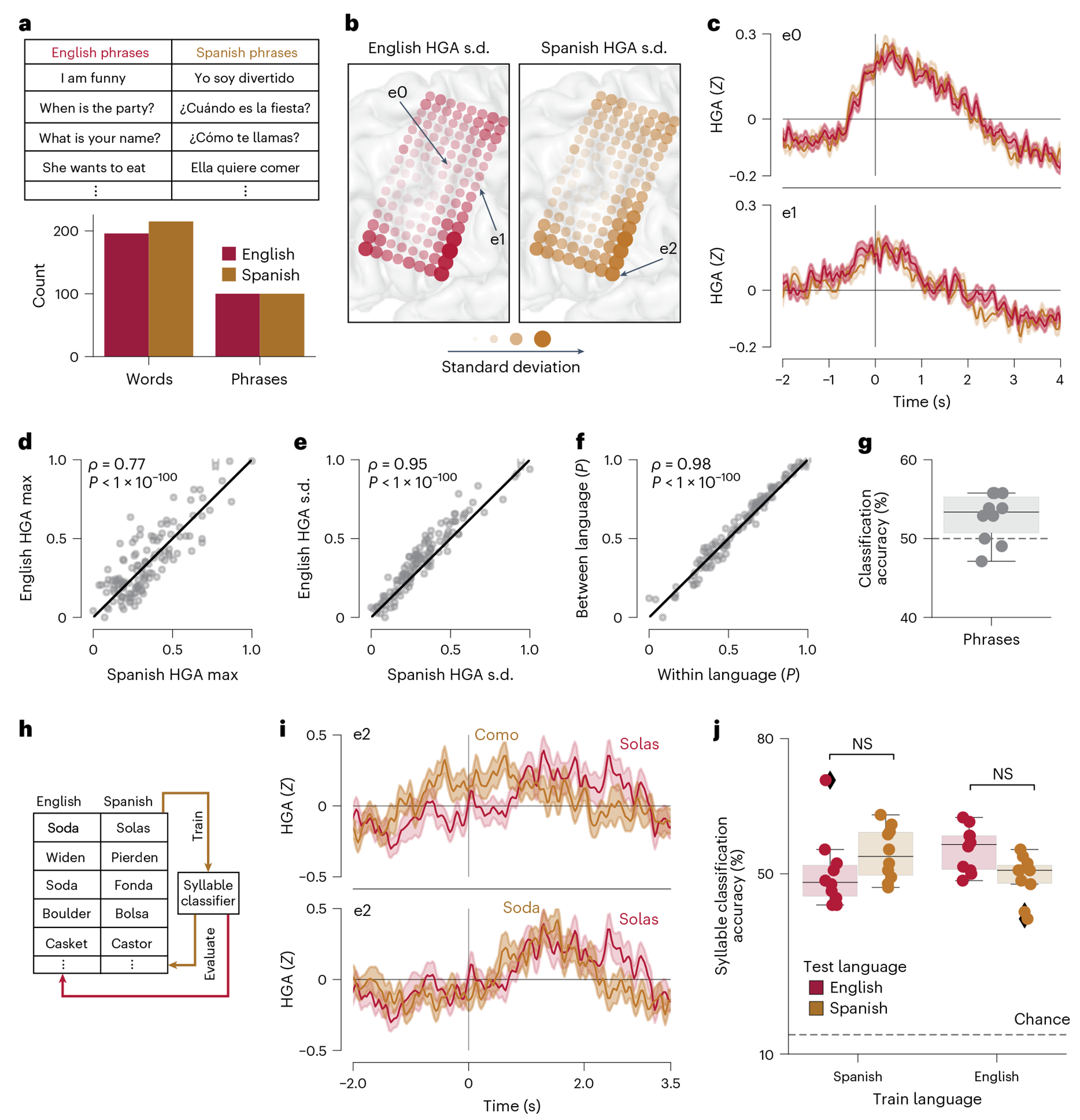
a, Large stimulus set of unique words and phrases used to cover a more comprehensive articulatory space in each language, relative to the vocabulary used for phrase-decoding (Fig. 1). b, Standard deviation of the average HGA from 0 to 2 s (relative to the visual ‘go’ cue) for English and Spanish phrases across each electrode. c, Sample ERPs to English and Spanish phrases for two electrodes noted in b. d, Relationship between the maximum HGA for each electrode during English and Spanish phrases. e, Relationship between the HGA standard deviation (as in b) for English and Spanish phrases for each electrode. f, Relationship of the correlation of ERPs within a language to the correlation of ERPs between languages for each electrode. d–f, Correlation assessed with non-parametric Spearman rank correlation and permutation testing over 128 electrodes (****P < 0.0001). Values normalized to fall between 0 and 1. g, 10-fold CV classification accuracy for classifying each phrase as English or Spanish. h, Stimulus set designed to probe a shared syllable representation between languages. We trained classifiers in each language and tested in both the same and the other language. i, Sample ERPs from an electrode indicated in b for different syllables in the same language and a shared syllable in different languages. j, 10-fold CV syllable-classification accuracy across training and testing paradigms. Two-sided Mann–Whitney U-test (NS, P = 0.082 and P = 0.025 for models trained on Spanish and English, respectively). c,i, Shaded regions indicate the standard error of the mean at each timepoint, computed across trials. In g and j, distributions are over 10 non-overlapping folds. Boxplots in all panels depict median (horizontal line inside box), 25th and 75th percentiles (box), 25th and 75th percentiles ±1.5 times the interquartile range (whiskers) and outliers (diamonds).

To better understand whether the temporal dynamics of neural responses differed between languages, we correlated HGA ERPs computed from trials in the same language with ERPs computed from trials in the other language. Again, we found a strong positive relationship between correlations within and between languages across electrodes (P < 0.0001, ρ = 0.98, non-parametric correlation permutation test; Fig. 3f). Finally, we trained a deep-learning model that predicted whether a phrase was English or Spanish on the basis of the neural features, HGA and LFS, during the speech attempt. We achieved 53.3% median 10-fold CV classification accuracy (Fig. 3g; 99% CI: 49.0, 55.8%), indicating that performance was not different from chance. Therefore, across a large phrase set, the precise temporal patterns of neural features in the speech-motor cortex also cannot strongly distinguish between languages.

Shared syllable representations enable cross-language training and testing of classifiers

It is hypothesized that bilinguals who learn L2 later in life may fit the articulatory content of L2 into previously learned L1 representations. One way this may manifest is in a shared syllable representation across languages^30,39,40. Given the strong evidence for shared articulatory representations with our participant, we assessed whether a syllable classifier could generalize between English and Spanish. We designed an utterance set in which the same 7 syllables were present in 7 English and Spanish words (Fig. 3h and Supplementary Table 8). ERPs from a sample electrode demonstrate a clear similarity in neural activity for the same syllable across languages (Fig. 3i). Next, we trained syllable-classification models over the shared syllable set using neural data recorded as the participant attempted to say the English or Spanish words. We evaluated these models either on held-out data from the same language or data from the other language. Our syllable classifier achieved high performance regardless of whether training and testing occurred in the same language (Fig. 3j; P = 0.08 and P = 0.03, two-sided Mann–Whitney U-test, for train English (Spanish) and test Spanish (English), respectively). This provides compelling evidence that a shared syllable representation can allow data collected in one language to be repurposed for a second language.

Rapid transfer learning between languages

Transfer learning is a common technique in machine learning that involves the initialization of model weights with parameters learned on a separate task or dataset^55,56. Transfer learning has primarily been used in neural decoding to leverage models trained in previous participants to expedite training in a new participant^57,58.

Given strong shared articulatory representations between languages, we hypothesized that transfer learning between different languages in the same participant should expedite learning a new vocabulary. To assess this, we evaluated a potential use case where models trained on a vocabulary in a first language were used to learn a new vocabulary in a second language. We benchmarked this performance against a scheme in which models trained on a vocabulary in the first language were used to learn a new vocabulary in the same first language. We pre-trained English and Spanish models on 4.33 h of data from a vocabulary of 25 words in each respective language (for an analysis of how the amount of pre-training data affects transfer learning, see Supplementary Fig. 1). We then fine-tuned and tested these models on a new set of 25 Spanish words (Fig. 4b). Interestingly, we found that pre-training on an English vocabulary achieved equivalent performance to pre-training in Spanish. Further, we achieved significantly higher performance on the new vocabulary using either pre-training scheme, compared with no pre-training, after just minutes of new training data. We observed an analogous outcome when we fine-tuned and tested pre-trained models on a new set of 25 English words (Fig. 4c). Overall, this demonstrates that decoder training with a vocabulary in a new language can be expedited by leveraging previous data collected in a different language, minimizing required training times for multilingual BCI use.

Fig. 4 |. Rapid transfer learning between languages.

a, Schematic depiction of the paradigm used to evaluate transfer learning between languages. Models were trained on an English or Spanish vocabulary. These models were then fine-tuned and evaluated on a new English or Spanish vocabulary. b, Median classification accuracy as a function of amount of training data (learning curves) for fine-tuning and evaluating on a new Spanish vocabulary. c, Median classification accuracy as a function of amount of training data (learning curves) for fine-tuning and evaluating on a new English vocabulary. In b–c, models were either not pre-trained or pre-trained on a different English or Spanish vocabulary. Chance decoding level is 4%. d, Schematic depiction of the paradigm used to evaluate the effect of acoustic similarity between the train and fine-tune set on transfer learning efficacy. e, MCD (as in Fig. 2g) between each word in the acoustically (acou.) similar or different train sets with the corresponding word in the fine-tune/test set (**P = 0.0039; two-sided Wilcoxon signed-rank test). Distributions are over 10 words. f, Median classification accuracy as a function of amount of training data (learning curves) for fine-tuning and evaluating on the ‘fine-tune and test set’, defined in d, with transfer learning from the acoustically (acou.) similar and different models. Learning curves are also shown for no pre-training and transfer learning from a model trained on a semantically (sem.) similar set of words. Performance at 0.0 h of training data reflects the pre-trained model’s ability to generalize to the fine-tune and test set with no additional or specific training data. Chance decoding is 10% (dashed line). In b, c and f, the shaded areas represent 99% CI. Boxplots in e depict median (horizontal line inside box), 25th and 75th percentiles (box), 25th and 75th percentiles ±1.5 times the interquartile range (whiskers) and outliers (diamonds).

To further explore the factors that drove transfer learning and whether models could generalize to an entirely new vocabulary with no additional training data, we designed a new 10-word fine-tune and test set (Fig. 4d). We next designed three pre-training sets by choosing a word to pair with each of the 10 words in the test set that was either acoustically (acou.) similar, acoustically different, or semantically (sem.) similar (Fig. 4d). We verified that the pairwise MCD between each word in the acoustically similar set and the corresponding word in the test set was significantly lower than that of the acoustically different set and the test set (Fig. 4e; P = 0.004, two-sided Wilcoxon signed-rank test). We then computed learning curves on the new test set using transfer learning from one of the three pre-training sets or no transfer learning (Fig. 4f). Here we also included an evaluation point at 0 h of training data, which indicates the ability of the pre-trained model to generalize with no additional data specific to the fine-tune set. Notably, we see that only in the case of an acoustically similar pre-training set is this possible and learning curves with the acoustically similar set increase most rapidly (Fig. 4f). Overall, this demonstrates that careful design of pre-training and fine-tune/test sets for acoustic, and by virtue articulatory^2,54, similarity may allow generalization of models to bilingual vocabularies with as little as no additional training data.

Discussion

We leveraged shared articulatory representations in the speech-motor cortex to drive a bilingual speech neuroprosthesis. We achieved low word error rates, usable in a clinical setting⁵⁹, with high language-classification accuracy when the target language is freely decoded on the basis of neural features and, importantly, differential linguistic context that builds throughout a phrase. Over 1,300 days after implantation, our ECoG-based neural-classification algorithms demonstrate stable performance without retraining for over 40 days. We also observed robust decoding of syllables in a given language after training on data collected exclusively in the other language. Correspondingly, transfer learning between languages facilitated learning of a new vocabulary in a second language with as little as 1 h of new training data. Together, this set of findings parallels advancements in automatic speech recognition, bringing communication technology to multilingual and non-English speakers^60–62.

Notably, the participant learned Spanish natively (L1) and then learned English (L2) later in his adult life, after any critical acquisition period⁶³. However, we did not find any cortical regions or patterns of neural activity^26,28 in our coverage specific to English or Spanish speech attempts. Despite later acquisition of L2 (around time of the participant’s brainstem stroke), we also did not notice clear differences in magnitude of evoked activity between L1 and L2, noted in non-invasive neurophysiology studies^29–34. Aligning with theories that articulatory representations of L2 in the brain leverage those of L1 (refs. 39,40), our results demonstrate a largely conserved syllable representation between languages.

This shared articulatory representation offers key advantages for multilingual BCIs. BCIs typically require training data with the user to develop high-performance decoders. This puts a burden on the user, and long training times may discourage adoption and continued use^64,65. Here we demonstrate that, through transfer learning, training time for multilingual participants to use all their languages may be greatly reduced. Further, our sublexical decoders achieved robust performance on syllables in a new language with no additional language-specific training data. These findings suggest that future multilingual speech BCIs may target shared sublexical units (for example, phonemes¹⁴) to improve bilingual vocabulary sizes and decoding speeds, leveraging alternative approaches to fixed-window word decoding^8,15,66.

While being a single-participant study is a limitation of this work, the strength of shared cortical articulatory representations, despite the participant learning L2 later in adult life, is encouraging for generalizability to other patients. This is especially true for those who learned L2 early in life, which correlates with stronger shared representations^30,31,33,35. Future work, however, should examine whether this effect varies with L2 proficiency, age of acquisition and articulatory similarity to L1. Though this study leveraged invasive electrophysiology, these results also hold relevance for non-invasive BCIs. A potential advantage of non-invasive BCIs is the ability to sample a larger area of cortex involved in functions beyond speech-motor control. Non-invasive BCIs may apply a similar framework, as applied here with articulatory features, for higher-level language features, such as semantics^6,68, that could further enable rapid generalizability across languages. These studies may also find language-specific signals, which we did not see in the speech-motor cortex, but may exist in higher-order cortical regions^28,69,70. A complementary direction for invasive BCIs is to understand whether language-specific signals exist at the level of single neurons.

Needing to build linguistic context to decode the intended language is one limitation of this study. While we demonstrated a strong, shared articulatory representation between English and Spanish, it is possible that languages in different families, such as English and a tonal language (for example, Mandarin), have distinct cortical representations for certain speech-production features, such as pitch^71,72. These differences could improve neural decoding of the intended language but limit transfer learning between the languages. In addition, we modelled language selection at the phrase level. In practice, multilingual speakers may switch between languages within phrases (code-switching), a topic that has been studied with non-invasive neural recordings and large language models^73–75. Future studies may explore a neural code-switching signal or utilize code-switching language models to decode language at the word level⁷³. Overall, this study demonstrates the feasibility of a bilingual speech neuroprosthesis that can flexibly decode speech in the user’s intended language and generalize between languages with minimal training data, with the potential to restore more natural communication to the many bilinguals with paralysis who may benefit.

Methods

Clinical-trial overview and the participant

This study was conducted as part of the BCI Restoration of Arm and Voice (BRAVO) clinical trial (ClinicalTrials.gov; NCT03698149) approved by the US Food and Drug Administration (FDA), UCSF Institutional Review Board and the National Institutes of Health. This study was performed in accordance with the Declaration of Helsinki. The adult participant provided written informed consent to participate in this study. All ethical regulations were followed. This clinical trial is a phase 1 single-centre early feasibility study to evaluate the potential of ECoG-based neural interfaces for controlling advanced neuroprostheses that restore motor and communicative functions. Due to the exploratory nature of this trial and the limited number of trial participants, we did not pre-define specific secondary outcomes. Our primary endpoint, which was pre-defined, was to assess the efficacy of the trial and was stated in the protocol as ‘Feasibility of control of a wearable exoskeleton device and communication interface’. As such, a variety of analysis methods were applied with the trial participant throughout the trial, with the aim to fully assess the efficacy of an ECoG-based neural interface for motor and communication restoration. The data herein presented are not aimed at informing concrete conclusions regarding the primary outcomes of the trial. The study protocol passed approval of the Committee on Human Research at the University of California, San Francisco, and the FDA awarded an investigational device exemption for the ECoG neural implant used in this trial participant. Before completion of the trial, results of this work were agreed to be released by the data safety monitoring board.

The participant (he/him) involved in this study was 36 years old at enrolment. He was previously diagnosed with severe spastic quadriparesis and anarthria by neurologists and a speech-language pathologist due to stroke of the bilateral pons¹³. His injury did not affect cognitive function, and he has slight residual function of the vocal tract allowing for audible grunts and moans; however, he is unable to produce intelligible speech (Supplementary Note 1). To communicate, he relies on an Augmentative and Alternative Communication (AAC) interface that utilizes residual head movements to spell out words (Supplementary Note 2). After details concerning the neural implant, experimental protocols and medical risks were explained, the participant provided full informed consent to partake in the study. The participant is a native Spanish speaker (L1) and learned English in adult life, reaching fluency at age 30, after his brainstem stroke.

Neural implant

The participant’s neural implant was a high-density ECoG array (PMT) coupled with a percutaneous connector (Blackrock Microsystems). A total of 128 electrodes, arranged in a lattice formation, with 4-mm centre-to-centre spacing make up the ECoG array. Over 3 years ago, the array was surgically implanted on the pial surface of the left hemisphere. The array was centred to sample cortical regions essential for speech production, namely, the dorsal posterior aspect of the inferior frontal gyrus, the posterior aspect of the middle frontal gyrus, the precentral gyrus and the anterior aspect of the postcentral gyrus. To transmit data to a computer for further analysis, the percutaneous connector was implanted in the skull. The connector conducts electrical signals from the ECoG array to a detachable digital headstage and cable (NeuroPlex E, Blackrock Microsystems), which transmits the data to a computer with little signal processing. The device was implanted in February 2019 at the UCSF Medical Center without any surgical complications.

Data acquisition and pre-processing

To acquire and extract meaningful neural features for downstream analysis, we applied a multistep pipeline. First, the local field potential (LFP) was acquired from each electrode via a headstage (a detachable digital connector; NeuroPlex E, Blackrock Microsystems) connected to the percutaneous pedestal connector. The connector digitizes the LFP from each electrode and transmits the signals through an HDMI connection to a digital hub (Blackrock Microsystems). The digital hub relays the digitized signals to a Neuroport system (Blackrock Microsystems) through an optical fibre cable. The Neuroport system applies noise cancellation and an anti-aliasing filter to the signals before streaming them at 1 kHz to a separate online computer via an Ethernet connection (Colfax International). We used the NeuroPort Central Suite software package (v.7.0.4, Blackrock Microsystems) to control the Neuroport system.

The resulting LFP across electrodes was further processed on the online computer using a custom Python software package (rtNSR) that is capable of processing and analysing the ECoG signals, executing the online tasks, performing online decoding, and storing the data and task metadata^4,13,42,76. Common average referencing (CAR) is a useful technique for reducing shared noise across multichannel neural datasets⁷⁷. We used rtNSR to first apply a CAR (across all electrode channels) to each time sample of the ECoG LFP. We then extracted two sets of neural features from the re-referenced ECoG signals: HGA and LFS. To extract these features, we used digital finite impulse response filters to compute the analytic amplitude of the signals in the high-gamma frequency band (70–150 Hz; HGA) and an anti-aliased version of the signals (with a cut-off frequency at 100 Hz; LFS). We concatenated the time-aligned HGA and LFS into a single temporal stream, sampled at 200 Hz. The HGA was then derived from the analytic amplitude, whereas LFS was not. We next z-scored the HGA and LFS for each channel using a 30-s sliding window approach. Lastly, we rejected artefacts in the signal, defined as timepoints with 32 features with z-score magnitudes greater than 10. Each of these timepoints was replaced with the z-score values from the preceding timepoint and ignored when updating the 30-s window z-score statistics. These final, processed features defined the HGA and LFS used in subsequent analyses and online decoding (together referred to as ‘neural features’). All data collection and online decoding tasks were performed in a small office near the participant’s residence. To train decoding models and perform offline analyses, data were uploaded to the lab’s server infrastructure and models were trained using NVIDIA V100 GPUs hosted on this infrastructure.

Task design

To develop a system capable of online decoding of English and Spanish phrases, we collected two general types of tasks with the participant: an isolated-target task and a phrase-decoding task.

Isolated-target task

During the isolated-target task, the text for a target word appeared on the screen along with 4 dots on either side. The dots sequentially disappeared and the text target turned green to indicate that the participant should attempt to speak the word (‘go’ cue). The participant attempted to speak the target word at the ‘go’ cue. We first collected a version of the task where the participant was asked not to attempt to vocalize (mimed). Data included in this paper are from a subsequent version of the task where the participant was allowed to attempt audible grunts of the target word (overt). During the isolated-target task, we used a vocabulary of 104 words: 50 Spanish, 51 English and 3 that are shared across languages (referred to together as ‘bilingual words’; Supplementary Table 1). Neural data collected during the isolated-target task were used to train and optimize classification and detection models that were later used, without recalibration, for phrase decoding.

Phrase-decoding task

The phrase-decoding task is treated in detail in the Results section and Fig. 1a. In brief, the participant used this paradigm to either perform a copy-typing task with the bilingual test phrases (Supplementary Table 3) or freely use bilingual words to have a conversation. To choose bilingual test phrases and train language models (see below), we crowdsourced generation of a large set of phrases made from the bilingual words through volunteers independent of our laboratory. Similar to our previous work¹³, to form the bilingual test phrases, we chose 28 English and Spanish phrases at random that covered the entire vocabulary, had no grammatical errors and appeared at least 2 times in the generated corpus. Data collected during the phrase-decoding task were used for evaluation only, with no calibration of models or hyperparameters based on the bilingual test phrases.

Large bilingual-phrase set

To further probe the representation of English and Spanish speech attempts, we designed a large bilingual-phrase set with ~200 unique words in each language (Fig. 3a). These phrases were designed to span a large articulatory space in each language (Extended Data Fig. 10 and Supplementary Methods 1). These phrases were presented to the participant using a sliding cued paradigm. In brief, the participant first heard an audio version of the phrase. The text corresponding to the phrase was then shown on the screen. A green vertical bar then slid across the phrase at the same rate as the previously presented audio. The green vertical sliding bar indicated the timing of when the participant should attempt each word in the phrase. The neural data collected during this task were used offline to evaluate the representations of English and Spanish speech attempts on the speech-motor cortex. No online demonstrations were performed with this task paradigm and phrase set.

English and Spanish paired-syllable words

To probe a shared syllable representation between English and Spanish words, we designed a limited set of stimuli where each word shared a syllable, in a different context, with a word in the opposite language (Supplementary Table 8). We collected this set using a modified paradigm similar to the isolated-target task. In brief, the participant first heard an audio recording of each word. Next, the text corresponding to the target word appeared on the screen along with 4 dots on either side. The dots sequentially disappeared and the text target turned green to indicate that the participant should attempt to speak the word. The neural data collected during this task were used offline to train and test syllable classifiers between languages. No online demonstrations were performed with this task paradigm and phrase set.

Modelling

We trained speech detection and classification models using data collected during the isolated-target task where the participant attempted to speak bilingual words.

For use with the phrase-decoding task, trained models were saved to the online computer. Models were trained and implemented using the PyTorch Python package (v.1.6.0). Natural-language models were also used to encourage the system to decode plausible sequences of words in each language, complementing neural predictions during the phrase-decoding task (Supplementary Methods 2). All hyperparameters for phrase decoding were chosen and optimized on simulations with the isolated-target task, collected before evaluation (Supplementary Methods 3). We used common scientific computing packages in Python including NumPy, scikit-learn, pandas, seaborn and matplotlib for modelling and data analysis.

Speech detection

To allow the participant to volitionally engage and disengage the decoding system, we trained a speech detection model to detect attempted speech from neural features online. The speech detector was trained using both LFS and HGA at 200 Hz, using recurrent neural networks (in particular, long short-term memory layers) and truncated back-propagation through time, similar to previously described methods^13,42. Model architecture and training parameter details are listed in Supplementary Table 9.

In this work, we trained the model on overt isolated-target bilingual-words data and rest blocks (where the participant rested silently for 1 min). For each isolated-target bilingual-words block, we labelled each timepoint as ‘rest’, ‘speech preparation’ or ‘speech.’ Timepoints between the presentation of the target word on the screen and the ‘go’ cue were labelled as ‘speech preparation’ and timepoints between the ‘go’ cue and 2 s after the ‘go’ cue were labelled as ‘speech’. This window was chosen on the basis of the duration of average neural responses during speech attempts. Timepoints from 2 s after the ‘go’ cue to the end of the trial (when the screen cleared) were discarded from training due to the ambiguity of when a speech attempt truly ended and the participant was at rest. All other timepoints (that is, the 1 s between trials when the screen was blank) were labelled as ‘rest’. For rest blocks, every timepoint was labelled as ‘rest’. Rest blocks were added into the training set to augment the amount of timepoints when the participant was truly resting outside the task context.

The speech detector was trained using all available isolated bilingual-words data before online testing. This means that before each day of online testing, the speech detector was retrained if new isolated data were collected the previous day. The speech detector generates the probability of a speech event (causally) and thresholding converts these continuous probability streams into discrete events^13,42. Detection thresholding parameters (smoothing, probability thresholding and time thresholding) were manually fine-tuned by evaluating on held-out bilingual-phrase blocks that were not used in any part of the training of the speech detector.

Classification

We trained an artificial neural network (ANN) with the objective of classifying the neural features from a speech attempt as one of the 104 words in the bilingual-words set. During model training, we used stochastic gradient descent and the Adam optimizer⁷⁸ to find a set of parameters that minimized the cross-entropy loss between target and predicted outputs across the 104 classes. Weights were initialized with parameters learned on the previous collection of mimed bilingual words, given a small final improvement on overt with transfer learning from mimed (Supplementary Fig. 2).

In brief, the ANN processed a 3.5-s window of neural features (0–3.5 s relative to the ‘go’ cue) corresponding to a speech attempt. A 3.5-s window was chosen for the window length, as it was the speed at which the participant could reliably attempt sequential words using the cued decoding system. The neural features were first decimated by a factor of 6 to an effective rate of 33.33 Hz. A one-dimensional temporal convolutional layer further downsampled the neural features by a factor of 4. The downsampled neural features were then passed through a three-layered bidirectional gated recurrent neural network (GRU)⁷⁹. Here, dropout was used to prevent the model from overfitting. Finally, the output of the final timestep of the last layer of the GRU was passed through a dense, fully connected layer to produce 104 outputs corresponding to each word of the bilingual words. A softmax function was applied to these outputs to yield an estimated probability for each word. During training, the outputs corresponding to words in a different language from the target word were masked before computation of the loss. This encouraged the model to make predictions consistent with the vocabulary of each language. During evaluation, where the language of the speech attempt was unknown, we separately passed forward English and Spanish word probabilities to downstream decoding modules. See Supplementary Methods 3 for specific details regarding data augmentation and hyperparameter optimization. A table providing optimal hyperparameters is provided in Supplementary Table 10.

During the phrase-decoding task, we utilized model ensembling to minimize overfitting and variance caused by random initialization of parameters⁸⁰. We trained 10 distinct classification models using ten random subsets of the isolated-target task training set. Each model retained the same architecture but saw a slightly different distribution of training data. To evaluate a given window of neural features, we averaged predictions across the ten models to yield a single ensemble prediction.

Language modelling

We trained 5-gram natural-language models for both English and Spanish from the crowdsourced corpus using custom code (Supplementary Methods 2). Similar to previous work¹³, the language model was trained to output the probability of each word in the vocabulary on the basis of the preceding, up to 4 words in the sequence.

Phrase decoding

The primary goal of phrase decoding is to find the most likely sequence of words (s*) given neural data X. To solve this problem, we used a beam search approach similar to our previous work, with modifications to apply to word sequences in two languages^41,42. In brief, the neural features for each 3.5-s window were passed through the ensemble classifier to generate a neural-based probability for each word in the vocabulary. These probabilities were then split and rescaled into two vectors: one for Spanish words and the other for English words. At this stage, the same downstream decoding modules were applied separately for English and Spanish. The phrase decoding module finds s*, given its likelihood from the neural data and its likelihood under the language-model prior. At each window within the trial, the highest-scoring English beam was compared to the highest-scoring Spanish beam. The beam with the higher overall score was displayed to the participant as feedback and effectively set the language of the output. See Supplementary Methods 4 for a detailed mathematical treatment and information on hyperparameter selection for the beam search process.

System evaluation

During the phrase-decoding task, the participant was instructed to continue attempting each word in the phrase regardless of decoding accuracy. However, on a small subset of trials, the participant self-reported making an error or not being able to continue the attempt (n = 7 out of 168 total trials). Errors included attempting the wrong words in the phrase (n = 3, such as attempting in English rather than in Spanish), muscle spasms/shakes preventing attempted speech (n = 3) and having something in his eye (n = 1). Similar to our previous work with this participant⁴², we excluded these trials from subsequent analysis to focus on the performance of our system rather than the performance of the participant.

Word error rate

We report the WER as the sum of the word edit distances between the predicted and target phrases in a phrase-decoding block divided by the total number of words across all target phrases in the block. Each block contained 8 phrases: 4 English and 4 Spanish. Similar to previous studies, we chose to report WER over blocks, given that short phrases may become overly influential^42,43,76. To compute the WER in the neural-only condition, we left verbs unconjugated both in the decoded and ground-truth sentences, and considered results up to the point where the ground-truth and decoded sentences had the same number of words. Thus, it is the inverse of classification accuracy and allows us to probe the neural-classification performance of the system during the phrase-decoding paradigm.

Cross-validation accuracies

To evaluate the offline performance of our system in classifying bilingual words, we used 10-fold CV. In each of the 10 folds, 90% of the data was used for training and 10% for evaluation. Within the 90% of data used for training, 10% was randomly selected to be reserved for a validation set (used to early stop training, see Supplementary Methods 3). Within each of the 10 folds, we fitted 10 randomly initialized models to ensemble predictions on the held-out evaluation fold. When indicated, during evaluation, we masked the predictions that were not in the same language as the target word. This allowed us to probe performance over the English and Spanish vocabularies separately.

To assess performance over the full 104 bilingual-word vocabulary, we trained models with a single modification. We removed masking entirely to allow the models to learn associations across languages during training and testing. We also provide the CV accuracies for using different window sizes during classification of the full 104 bilingual-word vocabulary (Supplementary Fig. 3).

Performance without recalibration

To evaluate the performance of our system without daily recalibration, we trained a neural classifier using the same process as described above (Methods: Classification) on data collected before day 1,333 post-implantation. We then froze the weights of this classifier and evaluated its performance on isolated-task data collected on subsequent days until the start of online sentence decoding. We evaluated performance with the masking approach to compute accuracy over the English and Spanish vocabularies separately or the entire vocabulary. For a comparison, we used the same methodology to retrain the classifier, with sequential addition of each day’s data.

Electrode contributions to classification

To probe whether English and Spanish words led to similar electrode contributions, we trained classification models only on bilingual words in English or Spanish. We then evaluated the electrode contributions in these models to compare between the two languages. We defined the contribution of each electrode to classification performance as the derivative of the classifier’s loss function with respect to the input features (HGA or LFS) over time^13,42,81. This effectively measured the change in model outputs, given small changes in the HGA or LFS for each electrode across timepoints. To form a composite contribution per electrode and feature set, we calculated the L2-norm over time and averaged data across evaluation trials. For each feature set, we then log transformed the resulting values and normalized results so that each value fell between 0 and 1.

Confusability of English and Spanish words

To probe the confusability between bilingual words, we used the predictions from 10-fold CV models trained on all bilingual words with no masking. We computed a confusion matrix where each entry represents the number of times a word (row) was predicted as being any of the 104 words in the vocabulary. Intuitively, the entry on the diagonal then represents the number of times a word was correctly classified. We normalized each row to sum to 1, making each entry a proportion (0–1). To explore which factors drove confusability between any two words, we measured the semantic and acoustic similarity between bilingual words.

We first embedded each word as a 300-dimensional vector using Word2Vec⁵². We computed the semantic similarity between words as the cosine similarity between respective embedded vectors. We next generated an audio waveform for each word using a multilingual text-to-speech system⁸², where a single speaker was used. The MCD, commonly used to evaluate speech synthesis systems⁵³, was used to measure the acoustic similarity between words. The MCD was defined as the squared error between dynamically time-warped mel-cepstral coefficients of two waveforms.

A multiple-regression model was fitted to predict the confusability between every pair of bilingual words on the basis of whether the words were in the same language, as well as their semantic and acoustic similarity. To assess the relative variance explained by each factor, we removed each variable individually and calculated the drop in R² compared to the full model. We then normalized the three values for explained variance to sum to 1. To compute confidence intervals for these estimates, we sampled the confusion matrix with replacement 2,000 times. For each random sample, we performed the above-described procedure to compute the relative variance explained by each factor.

A shared articulatory representation across languages

To probe a shared articulatory representation, we first computed the standard deviation of the average HGA (0–2 s after a ‘go’ cue) for speech attempts to English and Spanish phrases within the large bilingual-phrase set. ERPs were calculated by averaging the HGA at each timepoint for speech attempts to phrases in each language. We computed the maximum HGA across timepoints of the ERP at each electrode.

We also tested the temporal correlations between the ERPs for English and Spanish phrases. During each iteration of 2,000 bootstraps, English and Spanish trials were randomly split into two equal groups. We then computed the ERPs for each group, resulting in 2 English and 2 Spanish ERPs per electrode. At each electrode, we computed the Pearson correlation between the ‘within language’ and ‘between language’ ERPs. The correlations across the ‘within’ and ‘between’ language groups were averaged to yield 2 data points per electrode per iteration. The median ‘between language’ and ‘within language’ correlation was taken across bootstraps for each electrode.

We next asked whether temporal patterns in the neural features could be used to classify each trial as an English or Spanish phrase. We fitted a classification model with the same parameters and architecture found optimal for bilingual words in the isolated-target task to predict whether a trial was an English or Spanish phrase on the basis of a time interval of (−2,4) s relative to the ‘go’ cue.

Syllable decoding

To decode syllables from speech attempts in the English and Spanish paired-syllable words set, we trained a classifier to predict syllable identity over the set of shared syllables (Supplementary Table 8). For syllables that occurred at the beginning of a word, we used neural features from a time window of (0,2) s relative to the ‘go’ cue. For syllables that occurred at the end of a word, we used neural features from a time window of (1.5,3.5) s relative to the ‘go’ cue. We then trained a classification model using the same architecture, training procedure (no masking) and hyperparameters (except that the dropout was lowered to 0.5, given fewer target classes) as found optimal for bilingual words in the isolated-target task to predict probabilities over the shared syllables. To evaluate the ability of classification models to generalize between languages, we used two evaluation schemes. To evaluate performance in the same language used to train the classifier, we used 10-fold CV. To evaluate performance on the other language not used in training, we used all syllable-pair trials from the non-training language (split into 10 equally sized folds).

Transfer learning between languages

To assess the efficacy of transfer learning between languages, we used data collected during the isolated-target task. We randomly selected 25 words from the English bilingual words and 25 words from the Spanish bilingual words. We then trained classification models for these vocabularies using the same architecture, training procedure (no masking) and hyperparameters as found optimal for bilingual words. This yielded two pre-trained models: one in English and the other in Spanish. We then randomly selected another 25 English words from the remaining unused English bilingual words to form a new vocabulary. We repeated the above-described process a second time, selecting 25 Spanish words from the remaining unused Spanish bilingual words to form the new vocabulary.

To compute learning curves with the new vocabulary, we used 10-fold CV. Within each fold, we iteratively trained classification models with increasing fractions of the training data. At each fraction of training data, we evaluated on the held-out evaluation fold. This yielded 10 estimates of evaluation accuracy at each fraction of training data included. We visualized the 99% confidence interval over these 10 estimates at each fraction of training data studied.

We computed learning curves on the new vocabulary using the above-described procedure under three conditions: no transfer learning (weights initialized randomly), transfer learning from the pre-trained English model, and transfer learning from the pre-trained Spanish model.

Statistics

We used two-sided non-parametric tests to compare groups of observations. For unpaired data, we utilized Mann–Whitney U-tests and for paired data, we used Wilcoxon signed-rank tests. We employed a cut-off of 0.01 to determine significance of P values and used a Holm–Bonferroni correction to adjust P values for multiple comparisons where the underlying neural data were not independent. Associated P values for the Spearman rank correlation were computed with permutation testing. Confidence intervals were computed using a bootstrapping approach. In brief, over 2,000 iterations, we randomly sampled the data (for example, blocks) with replacement and computed the desired metric (for example, the median word error rate over blocks). The 99% confidence interval was then taken over the bootstrapped distribution. To estimate the participant’s AAC rate, we ensured, using a Mann–Whitney U-test, that a subset of sentences that matched the distribution of all evaluation sentences was chosen (Supplementary Fig. 4 and Note 2).

Reporting summary

Further information on research design is available in the Nature Portfolio Reporting Summary linked to this article.

Extended Data

Extended Data Fig. 1 |. Timing and information flow through the bilingual-sentence decoding system.

Shown is a more detailed schematic overview of the bilingual-sentence decoding system to complement Fig. 1a. Three levels of information are depicted: the neural features, the decoding system, and the output to the participant monitor. To start, the participant makes a speech attempt. This is detected by the system and cues activation of an ongoing decoding process. Following activation, a series of 3.5 s windows are cued to the participant. At the end of each window, after the full 3.5 s have passed, the neural features from that window are passed to the decoding process illustrated in Fig. 1a. Following a latency to conduct the decoding, the most likely beam from the process in Fig. 1a is displayed on the participant monitor. This process continues to occur for sequential 3.5 s windows until a window with no detected speech occurs. After such a window, the decoding is finalized and terminated. The system then listens for another speech attempt to activate and repeat the process.

Extended Data Fig. 2 |. Graphical depiction of bilingual-word classification.

Shown is a schematic of the bilingual-word classification process. Neural features (256 total; 128 HGA and 128 LFS time series over 3.5 s) are classified as a word in the bilingual vocabulary. Neural features are first processed by a temporal convolution. Next, the features are passed through three bidirectional GRU layers. The latent state from these layers is then read out by a dense, linear layer that emits probabilities over the 104 words in the bilingual vocabulary. This process is performed by 10 distinct models, each with a different weight initialization and trained on different folds of the data. The probabilities generated across these 10 models are averaged to create one probability vector across the bilingual vocabulary. This vector is finally split by language and the probability for a given word is broadcast to all conjugated forms of the word before being combined with the language model, as shown in Fig. 1a.

Extended Data Fig. 3 |. Neural-only chance sentence-decoding performance.

Shown are neural-only specific chance sentence-decoding distributions, alongside the neural-only decoding performance shown in Fig. 1. Here, we specifically computed a chance distribution with respect to neural-only decoding. We did this by shuffling the neural features and passing them through the classifier. The chance error rate was then computed the same way as for neural-only performance (**** P < 0.0001; two-sided Mann-Whitney U-test with 3-way Holm-Bonferroni correction for multiple comparisons). Distributions are over 21 online phrase-decoding blocks. Box plots in all panels depict median (horizontal line inside box), 25th and 75th percentiles (box), 25th and 75th percentiles +/− 1.5 times the interquartile range (whiskers), and outliers (diamonds).

Extended Data Fig. 4 |. Performance of attempted speech model on silent reading and listening.

For a subset of 10 bilingual words, we collected neural features during attempted speech, passive listening, and silent reading (roughly 250 trials in each paradigm). A model was trained on attempted speech data, using the same procedure throughout the manuscript, and evaluated on neural features from held-out attempted speech, passive listening, and silent reading trials. Performance was not significantly different from chance when evaluating the attempted speech model on listening or silent reading, in contrast to evaluation on attempted speech. This provides evidence that attempted speech neural features are specific to motor production of speech and not reflecting a process that strongly underlies listening or silent reading. Results are from 10-fold cross validation within each paradigm. Dashed line indicates chance performance (10%). Box plots in all panels depict median (horizontal line inside box), 25th and 75th percentiles (box), 25th and 75th percentiles +/− 1.5 times the interquartile range (whiskers), and outliers (diamonds).

Extended Data Fig. 5 |. Classification accuracy over the full 104 bilingual-words.

a, Shown is unmasked classification accuracy over the full 104 bilingual-words. The classifier retained stable performance without retraining (weights frozen at black dotted line) as in Fig. 2b. b, Classification performance before and after a 30-day break in recording without retraining (P = 0.31, two-sided Mann-Whitney U-test). Distributions are over 5 days. c, 10-fold cross validation (CV) accuracy over the unmasked 104 bilingual-words using all collected data. Median CV accuracy 47.24% (99% CI: [45.83,48.23] %). Distributions are over 10 non-overlapping folds. Box plots in all panels depict median (horizontal line inside box), 25th and 75th percentiles (box), 25th and 75th percentiles +/− 1.5 times the interquartile range (whiskers), and outliers (diamonds).

Extended Data Fig. 6 |. Acoustic similarity of words within the English and Spanish bilingual words.

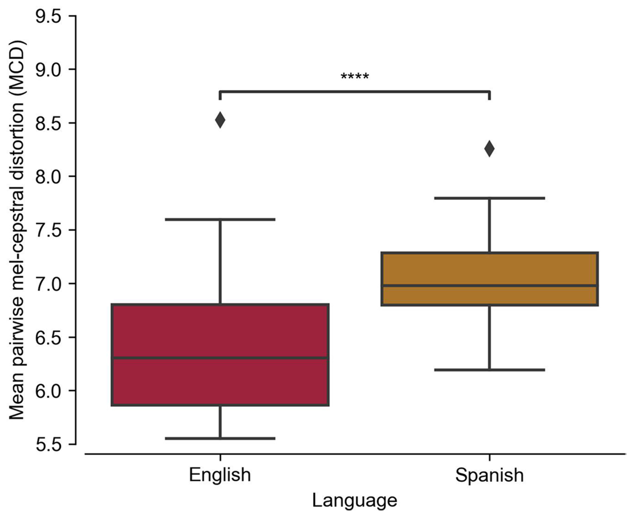
For each word in the English vocabulary we calculated the mean pairwise mel-cepstral distortion (MCD) to all other English words. We repeated the same procedure for Spanish. Distributions are over 51 English and 50 Spanish words (shared words were excluded). English words have a significantly lower mean pairwise MCD (**** P < 0.0001, two-sided Mann-Whitney U-test). This indicates that English words, on average, are more acoustically confusable with other English words than Spanish words are with other Spanish words. Box plots in all panels depict median (horizontal line inside box), 25th and 75th percentiles (box), 25th and 75th percentiles +/− 1.5 times the interquartile range (whiskers), and outliers (diamonds).

Extended Data Fig. 7 |. Effects of re-training models daily during frozen-decoder evaluation.

Shown is a comparison between performance with and without re-calibration. (a) Shown is the performance without re-calibration for reference taken from (Fig. 2b). (b) Shown is the performance with retraining the classifier with sequential addition of each day’s data. (c) Shown are distributions of accuracy with and without re-training, demonstrating that small improvements may be found with re-training the decoders with each day’s data. Distributions are over 9 days in each boxplot (starting after the first-day when retraining is possible). Chance is 1.85% for English, 1.89% for Spanish, and 1.87% for all words (masked). Box plots in all panels depict median (horizontal line inside box), 25th and 75th percentiles (box), 25th and 75th percentiles +/− 1.5 times the interquartile range (whiskers), and outliers (diamonds).

Extended Data Fig. 8 |. Distinct contributions of HGA and LFS to classifier performance.

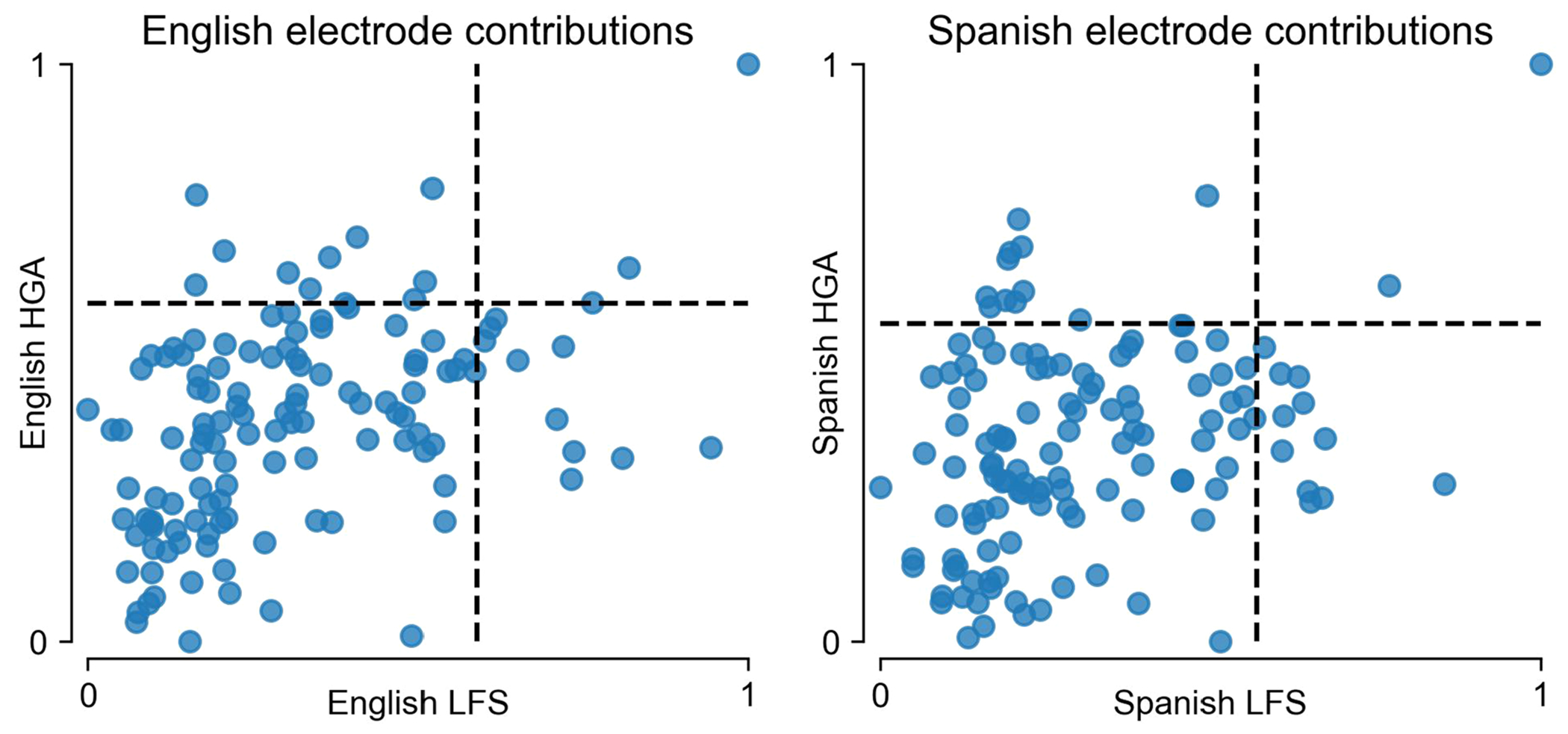
Shown are plots of electrode contributions for HGA against LFS, separately for English (left) and Spanish (right) trained models (as in Fig. 2d,e). The dotted lines indicate the 90th percentile of HGA and LFS contributions. The majority of electrodes only fall above the 90th percentile for one of HGA or LFS.

Extended Data Fig. 9 |. Full confusion matrix over all bilingual-words.

Full confusion matrix over the 104 bilingual-words. The sum of each row was normalized to 1, making confusion a proportion from (0-1). Predictions were generated using 10-fold cross validation over the full 104 bilingual-words with no masking (as in Extended Data Fig. 5).

Extended Data Fig. 10 |. Acoustic coverage of large-bilingual-phrase set.

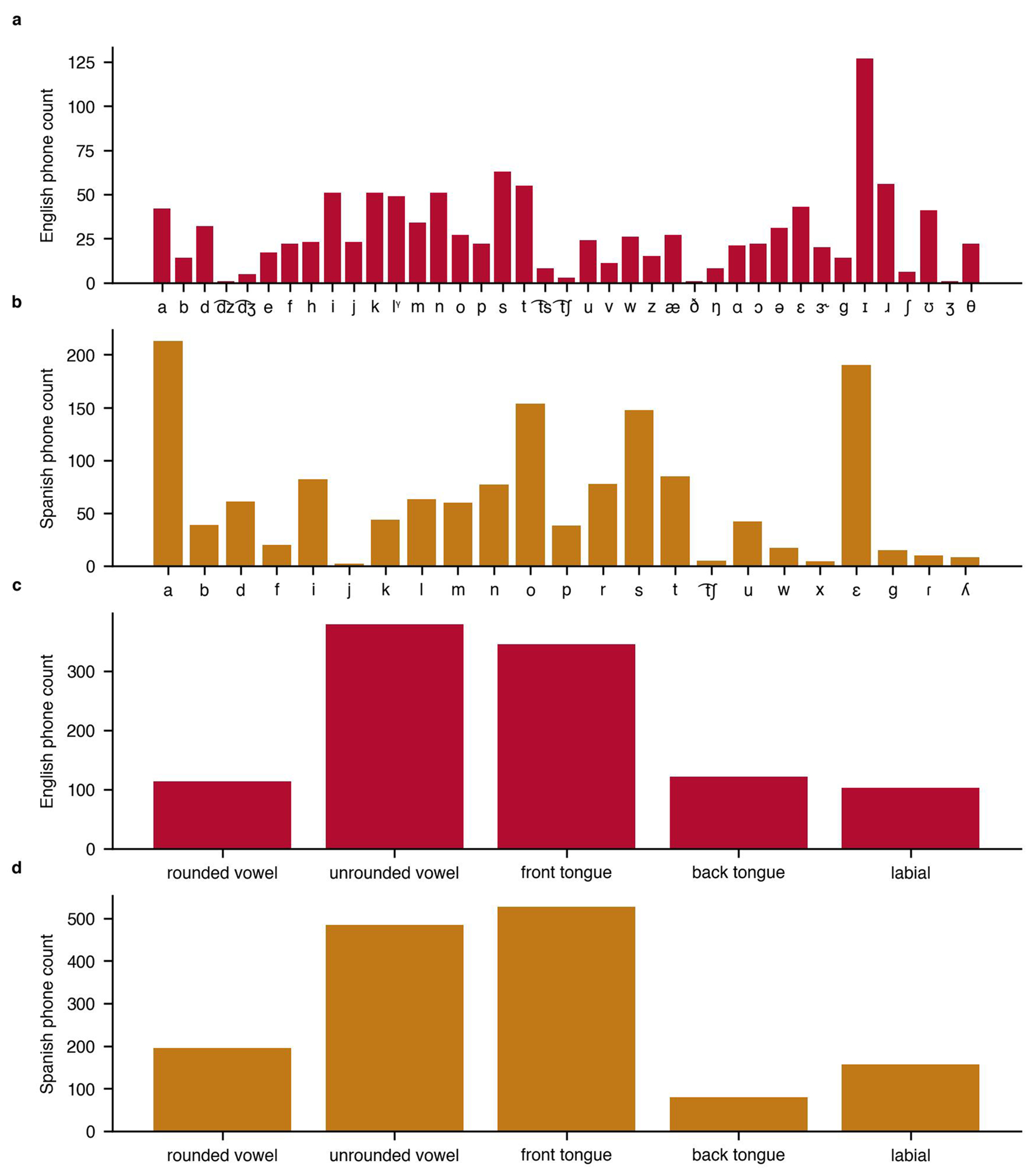
We quantified the distribution of phonemes and phoneme place of articulation features to ensure the large-bilingual-phrase set covered a broad space in each language. We designed the large-bilingual-phrase set to sample a broad range of English (a) and Spanish (b) phonemes. We ensured that the relative proportion of phoneme place of articulation features was similar between English (c) and Spanish (d).

Data availability

The data needed to recreate the main figures are provided as Source Data, and are also available in GitHub at https://github.com/asilvaalex4/bilingual_speech_bci. The raw patient data are accessible to researchers from other institutions, but public sharing is restricted pursuant to our clinical trial protocol. Full access to the data will be granted on reasonable request to E.F.C. at edward.chang@ucsf.edu, and a response can be expected in under 3 weeks. Shared data must be kept confidential and not provided to others unless approval is obtained. Shared data will not contain any information that may identify the participant, to protect their anonymity. Source data are provided with this paper.

References

- 1.Nip I & Roth CR in Encyclopedia of Clinical Neuropsychology (eds Kreutzer J et al. ) 1–1 (Springer, 2017). [Google Scholar]
- 2.Chartier J, Anumanchipalli GK, Johnson K & Chang EF Encoding of articulatory kinematic trajectories in human speech sensorimotor cortex. Neuron 98, 1042–1054.e4 (2018). [DOI] [PMC free article] [PubMed] [Google Scholar]
- 3.Herff C et al. Generating natural, intelligible speech from brain activity in motor, premotor, and inferior frontal cortices. Front. Neurosci 13, 1267 (2019). [DOI] [PMC free article] [PubMed] [Google Scholar]
- 4.Moses DA, Leonard MK, Makin JG & Chang EF Real-time decoding of question-and-answer speech dialogue using human cortical activity. Nat. Commun 10, 3096 (2019). [DOI] [PMC free article] [PubMed] [Google Scholar]
- 5.Soroush PZ et al. The nested hierarchy of overt, mouthed, and imagined speech activity evident in intracranial recordings. NeuroImage 269, 119913 (2023). [DOI] [PubMed] [Google Scholar]
- 6.Thomas TM et al. Decoding articulatory and phonetic components of naturalistic continuous speech from the distributed language network. J. Neural Eng 20, 046030 (2023). [DOI] [PubMed] [Google Scholar]
- 7.Stavisky SD et al. Neural ensemble dynamics in dorsal motor cortex during speech in people with paralysis. eLife 8, e46015 (2019). [DOI] [PMC free article] [PubMed] [Google Scholar]
- 8.Willett FR et al. A high-performance speech neuroprosthesis. Nature 620, 1031–1036 (2023). [DOI] [PMC free article] [PubMed] [Google Scholar]
- 9.Wandelt SK et al. Decoding grasp and speech signals from the cortical grasp circuit in a tetraplegic human. Neuron 110, 1777–1787.e3 (2022). [DOI] [PMC free article] [PubMed] [Google Scholar]
- 10.Angrick M et al. Speech synthesis from ECoG using densely connected 3D convolutional neural networks. J. Neural Eng 16, 036019 (2019). [DOI] [PMC free article] [PubMed] [Google Scholar]
- 11.Berezutskaya J et al. Direct speech reconstruction from sensorimotor brain activity with optimized deep learning models. J. Neural Eng 20, 056010 (2023). [DOI] [PMC free article] [PubMed] [Google Scholar]
- 12.Dash D, Ferrari P & Wang J Decoding imagined and spoken phrases from non-invasive neural (MEG) signals. Front. Neurosci 14, 290 (2020). [DOI] [PMC free article] [PubMed] [Google Scholar]
- 13.Moses DA et al. Neuroprosthesis for decoding speech in a paralyzed person with anarthria. N. Engl. J. Med 385, 217–227 (2021). [DOI] [PMC free article] [PubMed] [Google Scholar]
- 14.Mugler EM et al. Direct classification of all American English phonemes using signals from functional speech motor cortex. J. Neural Eng 11, 035015 (2014). [DOI] [PMC free article] [PubMed] [Google Scholar]
- 15.Metzger SL et al. A high-performance neuroprosthesis for speech decoding and avatar control. Nature 620, 1037–1046 (2023). [DOI] [PMC free article] [PubMed] [Google Scholar]
- 16.Choe J et al. Language-specific effects on automatic speech recognition errors for world Englishes. In Proc. 29th International Conference on Computational Linguistics 7177–7186 (International Committee on Computational Linguistics, 2022). [Google Scholar]
- 17.DiChristofano A, Shuster H, Chandra S & Patwari N Global performance disparities between English-language accents in automatic speech recognition. Preprint at http://arxiv.org/abs/2208.01157 (2023). [Google Scholar]
- 18.Baker C & Jones S Encyclopedia of Bilingualism and Bilingual Education (Multilingual Matters, 1998). [Google Scholar]
- 19.Athanasopoulos P et al. Two languages, two minds: flexible cognitive processing driven by language of operation. Psychol. Sci 26, 518–526 (2015). [DOI] [PubMed] [Google Scholar]
- 20.Chen SX & Bond MH Two languages, two personalities? Examining language effects on the expression of personality in a bilingual context. Pers. Soc. Psychol. Bull 36, 1514–1528 (2010). [DOI] [PubMed] [Google Scholar]
- 21.Costa A & Sebastián-Gallés N How does the bilingual experience sculpt the brain? Nat. Rev. Neurosci 15, 336–345 (2014). [DOI] [PMC free article] [PubMed] [Google Scholar]
- 22.Naranowicz M, Jankowiak K & Behnke M Native and non-native language contexts differently modulate mood-driven electrodermal activity. Sci. Rep 12, 22361 (2022). [DOI] [PMC free article] [PubMed] [Google Scholar]
- 23.Li Q et al. Monolingual and bilingual language networks in healthy subjects using functional MRI and graph theory. Sci. Rep 11, 10568 (2021). [DOI] [PMC free article] [PubMed] [Google Scholar]
- 24.Pierce LJ, Chen J-K, Delcenserie A, Genesee F & Klein D Past experience shapes ongoing neural patterns for language. Nat. Commun 6, 10073 (2015). [DOI] [PMC free article] [PubMed] [Google Scholar]
- 25.Dehaene S Fitting two languages into one brain. Brain 122, 2207–2208 (1999). [DOI] [PubMed] [Google Scholar]
- 26.Kim KHS, Relkin NR, Lee K-M & Hirsch J Distinct cortical areas associated with native and second languages. Nature 388, 171–174 (1997). [DOI] [PubMed] [Google Scholar]
- 27.Tham WWP et al. Phonological processing in Chinese–English bilingual biscriptals: an fMRI study. NeuroImage 28, 579–587 (2005). [DOI] [PubMed] [Google Scholar]
- 28.Xu M, Baldauf D, Chang CQ, Desimone R & Tan LH Distinct distributed patterns of neural activity are associated with two languages in the bilingual brain. Sci. Adv 3, e1603309 (2017). [DOI] [PMC free article] [PubMed] [Google Scholar]
- 29.Berken JA et al. Neural activation in speech production and reading aloud in native and non-native languages. NeuroImage 112, 208–217 (2015). [DOI] [PubMed] [Google Scholar]
- 30.Del Maschio N & Abutalebi J The Handbook of the Neuroscience of Multilingualism (Wiley-Blackwell, 2019). [Google Scholar]
- 31.DeLuca V, Rothman J, Bialystok E & Pliatsikas C Redefining bilingualism as a spectrum of experiences that differentially affects brain structure and function. Proc. Natl Acad. Sci. USA 116, 7565–7574 (2019). [DOI] [PMC free article] [PubMed] [Google Scholar]
- 32.Liu H, Hu Z, Guo T & Peng D Speaking words in two languages with one brain: neural overlap and dissociation. Brain Res. 1316, 75–82 (2010). [DOI] [PubMed] [Google Scholar]
- 33.Shimada K et al. Fluency-dependent cortical activation associated with speech production and comprehension in second language learners. Neuroscience 300, 474–492 (2015). [DOI] [PubMed] [Google Scholar]
- 34.Treutler M & Sörös P Functional MRI of native and non-native speech sound production in sequential German–English Bilinguals. Front. Hum. Neurosci 15, 683277 (2021). [DOI] [PMC free article] [PubMed] [Google Scholar]
- 35.Cao F, Tao R, Liu L, Perfetti CA & Booth JR High proficiency in a second language is characterized by greater involvement of the first language network: evidence from Chinese learners of English. J. Cogn. Neurosci 25, 1649–1663 (2013). [DOI] [PMC free article] [PubMed] [Google Scholar]
- 36.Geng S et al. Intersecting distributed networks support convergent linguistic functioning across different languages in bilinguals. Commun. Biol 6, 99 (2023). [DOI] [PMC free article] [PubMed] [Google Scholar]
- 37.Malik-Moraleda S et al. An investigation across 45 languages and 12 language families reveals a universal language network. Nat. Neurosci 25, 1014–1019 (2022). [DOI] [PMC free article] [PubMed] [Google Scholar]
- 38.Perani D & Abutalebi J The neural basis of first and second language processing. Curr. Opin. Neurobiol 15, 202–206 (2005). [DOI] [PubMed] [Google Scholar]
- 39.Alario F-X, Goslin J, Michel V & Laganaro M The functional origin of the foreign accent: evidence from the syllable-frequency effect in bilingual speakers. Psychol. Sci 21, 15–20 (2010). [DOI] [PubMed] [Google Scholar]
- 40.Simmonds A, Wise R & Leech R Two tongues, one brain: imaging bilingual speech production. Front. Psychol 2, 166 (2011). [DOI] [PMC free article] [PubMed] [Google Scholar]
- 41.Hannun AY, Maas AL, Jurafsky D & Ng AY First-pass large vocabulary continuous speech recognition using bi-directional recurrent DNNs. Preprint at https://arxiv.org/abs/1408.2873 (2014). [Google Scholar]
- 42.Metzger SL et al. Generalizable spelling using a speech neuroprosthesis in an individual with severe limb and vocal paralysis. Nat. Commun 13, 6510 (2022). [DOI] [PMC free article] [PubMed] [Google Scholar]
- 43.Willett FR, Avansino DT, Hochberg LR, Henderson JM & Shenoy KV High-performance brain-to-text communication via handwriting. Nature 593, 249–254 (2021). [DOI] [PMC free article] [PubMed] [Google Scholar]
- 44.Radford A. et al. Language models are unsupervised multitask learners. Preprint at Semantic Scholar https://www.semanticscholar.org/paper/Language-Models-are-Unsupervised-Multitask-Learners-Radford-Wu/9405cc0d6169988371b2755e573cc28650d14dfe (2018). [Google Scholar]
- 45.Blakely T, Miller KJ, Zanos SP, Rao RPN & Ojemann JG Robust, long-term control of an electrocorticographic brain–computer interface with fixed parameters. Neurosurg. Focus 27, E13 (2009). [DOI] [PubMed] [Google Scholar]
- 46.Pels EGM et al. Stability of a chronic implanted brain–computer interface in late-stage amyotrophic lateral sclerosis. Clin. Neurophysiol 130, 1798–1803 (2019). [DOI] [PMC free article] [PubMed] [Google Scholar]
- 47.Silversmith DB et al. Plug-and-play control of a brain–computer interface through neural map stabilization. Nat. Biotechnol 39, 326–335 (2021). [DOI] [PubMed] [Google Scholar]
- 48.Volkova K, Lebedev MA, Kaplan A & Ossadtchi A Decoding movement from electrocorticographic activity: a review. Front. Neuroinform 13, 74 (2019). [DOI] [PMC free article] [PubMed] [Google Scholar]
- 49.Luo S. et al. Stable decoding from a speech BCI enables control for an individual with ALS without recalibration for 3 months. Adv. Sci 10, 2304853 (2023). [DOI] [PMC free article] [PubMed] [Google Scholar]
- 50.Bouchard KE, Mesgarani N, Johnson K & Chang EF Functional organization of human sensorimotor cortex for speech articulation. Nature 495, 327–332 (2013). [DOI] [PMC free article] [PubMed] [Google Scholar]
- 51.Carey D, Krishnan S, Callaghan MF, Sereno MI & Dick F Functional and quantitative MRI mapping of somatomotor representations of human supralaryngeal vocal tract. Cereb. Cortex 27, 265–278 (2017). [DOI] [PMC free article] [PubMed] [Google Scholar]
- 52.Mikolov T, Chen K, Corrado G & Dean J Efficient estimation of word representations in vector space. Preprint at https://arxiv.org/abs/1301.3781v3 (2013). [Google Scholar]
- 53.Kubichek R. Mel-cepstral distance measure for objective speech quality assessment. In Proc. IEEE Pacific Rim Conference on Communications, Computers and Signal Processing 125–128 (IEEE, 1993). [Google Scholar]
- 54.Mitra V. et al. Joint modeling of articulatory and acoustic spaces for continuous speech recognition tasks. In 2017 IEEE International Conference on Acoustics, Speech and Signal Processing (ICASSP) 5205 (IEEE, 2017). [Google Scholar]
- 55.Caruana R. Multitask learning. Mach. Learn 28, 41–75 (1997). [Google Scholar]
- 56.Tan C. et al. A survey on deep transfer learning. In Artificial Neural Networks and Machine Learning – ICANN 2018 (eds Kůrkovã V et al. ) 270–279 (Springer, 2018). [Google Scholar]
- 57.Makin JG, Moses DA & Chang EF Machine translation of cortical activity to text with an encoder–decoder framework. Nat. Neurosci 23, 575–582 (2020). [DOI] [PMC free article] [PubMed] [Google Scholar]
- 58.Peterson SM, Steine-Hanson Z, Davis N, Rao RPN & Brunton BW Generalized neural decoders for transfer learning across participants and recording modalities. J. Neural Eng 18, 026014 (2021). [DOI] [PubMed] [Google Scholar]
- 59.Watanabe S, Delcroix M, Metze F & Hershey JR New Era for Robust Speech Recognition: Exploiting Deep Learning (Springer, 2017). [Google Scholar]
- 60.Gao H. et al. Domain generalization for language-independent automatic speech recognition. Front. Artif. Intell 5, 806274 (2022). [DOI] [PMC free article] [PubMed] [Google Scholar]
- 61.Radford A. et al. Robust speech recognition via large-scale weak supervision. Preprint at http://arxiv.org/abs/2212.04356 (2022). [Google Scholar]
- 62.Zhang Y. et al. Google USM: scaling automatic speech recognition beyond 100 languages. Preprint at http://arxiv.org/abs/2303.01037 (2023). [Google Scholar]
- 63.Hartshorne JK, Tenenbaum JB & Pinker S A critical period for second language acquisition: evidence from 2/3 million English speakers. Cognition 177, 263–277 (2018). [DOI] [PMC free article] [PubMed] [Google Scholar]
- 64.Huggins JE, Wren PA & Gruis KL What would brain–computer interface users want? Opinions and priorities of potential users with amyotrophic lateral sclerosis. Amyotroph. Lateral Scler 12, 318–324 (2011). [DOI] [PMC free article] [PubMed] [Google Scholar]
- 65.Peters B. et al. Brain–computer interface users speak up: the Virtual Users’ Forum at the 2013 International Brain-Computer Interface Meeting. Arch. Phys. Med. Rehabil 96, S33–S37 (2015). [DOI] [PMC free article] [PubMed] [Google Scholar]
- 66.Herff C. et al. Brain-to-text: decoding spoken phrases from phone representations in the brain. Front. Neurosci 9, 217 (2015). [DOI] [PMC free article] [PubMed] [Google Scholar]
- 67.Tang J, LeBel A, Jain S & Huth AG Semantic reconstruction of continuous language from non-invasive brain recordings. Nat. Neurosci 26, 858–866 (2023). [DOI] [PMC free article] [PubMed] [Google Scholar]
- 68.Correia J. et al. Brain-based translation: fMRI decoding of spoken words in bilinguals reveals language-independent semantic representations in anterior temporal lobe. J. Neurosci 34, 332–338 (2014). [DOI] [PMC free article] [PubMed] [Google Scholar]
- 69.Lucas TH, McKhann GM & Ojemann GA Functional separation of languages in the bilingual brain: a comparison of electrical stimulation language mapping in 25 bilingual patients and 117 monolingual control patients. J. Neurosurg 101, 449–457 (2004). [DOI] [PubMed] [Google Scholar]
- 70.Giussani C, Roux F-E, Lubrano V, Gaini SM & Bello L Review of language organisation in bilingual patients: what can we learn from direct brain mapping? Acta Neurochir. 149, 1109–1116 (2007). [DOI] [PubMed] [Google Scholar]
- 71.Best CT The diversity of tone languages and the roles of pitch variation in non-tone languages: considerations for tone perception research. Front. Psychol 10, 364 (2019). [DOI] [PMC free article] [PubMed] [Google Scholar]
- 72.Li Y, Tang C, Lu J, Wu J & Chang EF Human cortical encoding of pitch in tonal and non-tonal languages. Nat. Commun 12, 1161 (2021). [DOI] [PMC free article] [PubMed] [Google Scholar]
- 73.Lee G & Li H Modeling code-switch languages using bilingual parallel corpus. In Proc. 58th Annual Meeting of the Association for Computational Linguistics 860–870 (Association for Computational Linguistics, 2020). [Google Scholar]
- 74.Rossi E, Dussias PE, Diaz M, van Hell JG & Newman S Neural signatures of inhibitory control in intra-sentential code-switching: evidence from fMRI. J. Neurolinguist 57, 100938 (2021). [DOI] [PMC free article] [PubMed] [Google Scholar]
- 75.Zheng X, Roelofs A, Erkan H & Lemhöfer K Dynamics of inhibitory control during bilingual speech production: an electrophysiological study. Neuropsychologia 140, 107387 (2020). [DOI] [PubMed] [Google Scholar]
- 76.Moses DA, Leonard MK & Chang EF Real-time classification of auditory sentences using evoked cortical activity in humans. J. Neural Eng 15, 036005 (2018). [DOI] [PMC free article] [PubMed] [Google Scholar]
- 77.Ludwig KA et al. Using a common average reference to improve cortical neuron recordings from microelectrode arrays. J. Neurophysiol 101, 1679–1689 (2009). [DOI] [PMC free article] [PubMed] [Google Scholar]
- 78.Kingma DP & Ba J Adam: a method for stochastic optimization. Preprint at https://arxiv.org/abs/1412.6980 (2017). [Google Scholar]
- 79.Cho K. et al. Learning phrase representations using RNN encoder-decoder for statistical machine translation. Preprint at https://arxiv.org/abs/1406.1078 (2014). [Google Scholar]
- 80.Fort S, Hu H & Lakshminarayanan B Deep ensembles: a loss landscape perspective. Preprint at https://arxiv.org/abs/1912.02757 (2020). [Google Scholar]
- 81.Simonyan K, Vedaldi A & Zisserman A Deep inside convolutional networks: visualising image classification models and saliency maps. Preprint at https://arxiv.org/abs/1312.6034 (2014). [Google Scholar]
- 82.Lux F, Koch J, Schweitzer A & Vu NT The IMS Toucan system for the Blizzard Challenge 2021. Preprint at https://arxiv.org/pdf/2310.17499 (2021). [Google Scholar]
Associated Data
This section collects any data citations, data availability statements, or supplementary materials included in this article.
Supplementary Materials
Data Availability Statement