NEC-NET : Segmentation and Feature Extraction Network for the Neurocranium in Early Childhood

Abstract

In early life, the neurocranium undergoes rapid changes to accommodate the expanding brain. Neurocranial maturation can be disrupted by developmental abnormalities and environmental factors such as sleep position. To establish a baseline for the early detection of anomalies, it is important to understand how this structure typically grows in healthy children. Here, we designed a deep neural network pipeline NEC-NET, including segmentation and classification, to analyze the normative development of the neurocranium in T1 MR images from healthy children aged 12 to 60 months old. The pipeline optimizes the segmentation of the neurocranium and shows the preliminary results of age-based regional differences among infants.

1. INTRODUCTION

Abnormalities in neurocranial shape are a frequent indication of various developmental diseases, and early identification in young children can be a crucial diagnostic tool for these conditions. At birth, the neurocranium is made up of ossified bone tissue that has formed thin, bony plates.^{1, 2} The sutures and fontanelles, which consist of soft connective tissue, hold these plates together. This structure’s flexibility allows the neurocranium to change shape during birth and to adapt to brain development. The sutures close as the child ages, with the frontal, or metopic, suture closing first in the first year of life and the coronal and sagittal sutures following by the age of three.^{3, 4} The brain’s surface area and cortical thickness both grow quickly between 0 and 2 years of age. It has been demonstrated that during the first year of life, the brain’s surface area expands by a factor of about 1.80, with the occipital lobe experiencing the most growth.⁵ Between the ages of 0 and 9 months, the thickness of the occipital cortical region also increases quickly. The neurocranium undergoes alterations as a result of such brain expansion, growing quickly from 25% of adult size at birth to 90% of adult size by ages 4–5, whereas the brain achieves 95% of its final volume by ages 6 and 7.^{6, 7}

Because developmental disorders may affect neurocranial growth either directly (for example, through craniosynostosis) or indirectly (through abnormal brain growth or cerebrospinal fluid production, e.g. hydrocephalus), it is crucial to monitor this flexible architecture in infancy. Diseases like Paget’s disease, which causes bone deformities, craniosynostosis, in which sutures close prematurely in 1 in 2000 to 2500 live births, thalassemia, which is brought on by abnormal hemoglobin production, and large arteriovenous malformations all have an impact on skull thickness.⁸

Although computed tomography (CT) is the typical method used in hospitals to diagnose possible neurocranium pathologies in infants, it is not used to amass data from healthy infants given the potential negative long-term effects of its ionizing radiation. Therefore, the segmentation of magnetic resonance (MR) images can be used as a substitute to study large populations of healthy infants. Though previous work has focused on the analysis of regional cranial shape development,^{8, 9} segmentation of MR images has not yet been utilized. Here, we introduce deep neural networks to perform MR image edge segmentation of the neurocranium.

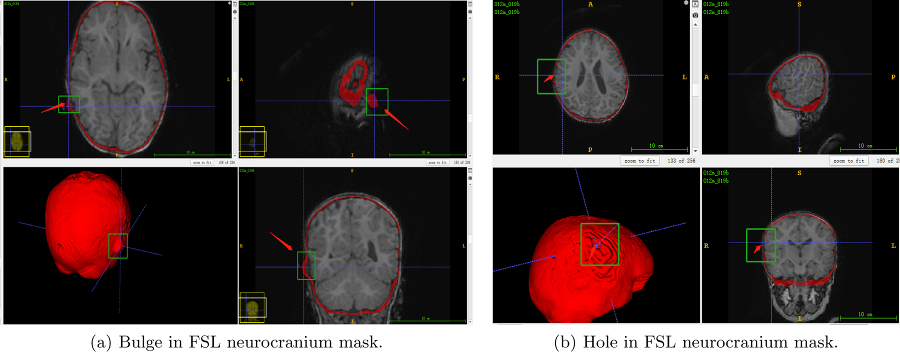
Accurate segmentation is the crucial first step in the analysis of neurocranial growth. Automated segmentation of the infant neurocranium is challenging due to the thinness of the structure, low image contrast, and rapid changes at those ages, requiring tight age fitting of training sets. Traditional automated segmentation software, such as FSL, produces neurocranial masks for this age group (see Fig.1), but they often need to be manually corrected, and in many cases, the algorithm fails completely. However, manual segmentation is time-consuming and costly. Convolutional neural networks (CNNs) have been successfully used in a variety of medical semantic segmentation applications since the development of deep learning, such as the segmentation of the brain, spine, acute brain hemorrhage, vessels, skull stripping in brain MRI, craniomaxillofacial bony structures, proximal femur, and cardiac images.^10–14 Medical images contain ample meaningful details; edges transmit shape information, whereas textures convey the appearance of regions. The CNN layers extract features (such as horizontal or vertical edges) from the training images during training, which enables the CNN to identify these features in subsequent images. Convolutional image filters are learned and altered in an automated process for a high-level description and a finer optimization process, giving CNNs an edge over other techniques.

Figure 1.

FSL neurocranium mask segmentation results. The FSL algorithm can result in bulges and holes in the mask (the red arrow and green box, respectively), leading to inaccurate segmentations.

We present a deep learning pipeline for evaluating infant brain development using masks of the neurocranium obtained from high resolution MRI brain images. An improved 3D U-Net¹⁵ is applied to perform the segmentation. CNN is also useful for classification,¹⁶ and we will use it to detect which neurocranial regions are involved in development. Using a CNN to produce meaningful heatmaps that emphasize the significance of specific voxel regions may be beneficial for showing neurocranium age-based differences. To improve the classification accuracy, the Gradient-weighted Class Activation Mapping (Grad-CAM) algorithm¹⁷ has been utilized. The method creates a coarse localization map that highlights the key areas in the image for concept prediction, by using the gradients of each target concept flowing into the final convolutional layer.

2. METHOD

2.1. Data

We use a sizable, pre-existing database of T1 MP-RAGE MRI scans (1.4–1.8 mm³) of healthy children acquired at the Baby Imaging Lab (https://www.babyimaginglab.com) to map normative neurocranial thickness in children between 12 and 60 months of age. The number of training subjects in each age group is shown in Table.1 and the number of test subjects in each age group is 2. Only singleton, full-term (37–42 weeks at birth) infants with no abnormalities on fetal ultrasonography and no known past neurological events or diseases were included. Informed consent was obtained from the parents of every participant, and Brown University’s Institutional Review Board authorized the study. A Siemens 3T Tim Trio scanner with a 12-channel head RF array was used to collect the data. Children were wrapped in a pediatric MedVac vacuum immobilization bag (CFI Medical Solutions, USA) and foam cushions while they slept to reduce intra-scan motion. By lowering the peak gradient amplitudes and slew rates, and employing a noise-insulating scanner bore insert, scanner noise was minimized (Quiet Barrier HD Composite, UltraBarrier, USA). Before pre-processing, all data were de-identified.

Table 1.

Number of subjects in training set by age.

Ages	12m	18m	24m	36m	48m	60m
Number	18	14	14	20	14	20

2.2. Preprocessing and Labeling

To train a precise segmentation model, we need to have accurate neurocranial brain labels. We first do some preprocessing steps, then revise the voxel region through manual correction. First, the data underwent the following pre-processing steps: To ensure consistency throughout processing, the MRI brain volume was first skull-stripped using FSL BET2 and resampled to a 1*1*1 mm³ resolution. The N4 ANTs bias correction tool was used to adjust for bias. Using FSL FLIRT with six degrees of freedom, the outcome was then linearly registered to a custom template that was age-matched. The same dataset that was described in¹⁸ was used to create this customized template, which was likewise resampled to a resolution of 1*1*1 mm³. The original T1-weighted image of the skull was then transformed into the template space.

The skull masks corresponding to the inner and outer skull tables were then created using the FSL Bet function. To check for correctness and remove overlapping voxels in the inner and outer cranium, each mask underwent a visual inspection and editing process. Frequently, the FSL results were not accurate enough which presented as bulges and/or holes in the neurocranium mask, such as the ones shown in Fig.1, so the segmentation needed to be changed manually.

2.3. Model Architecture

2.3.1. Segmentation Network

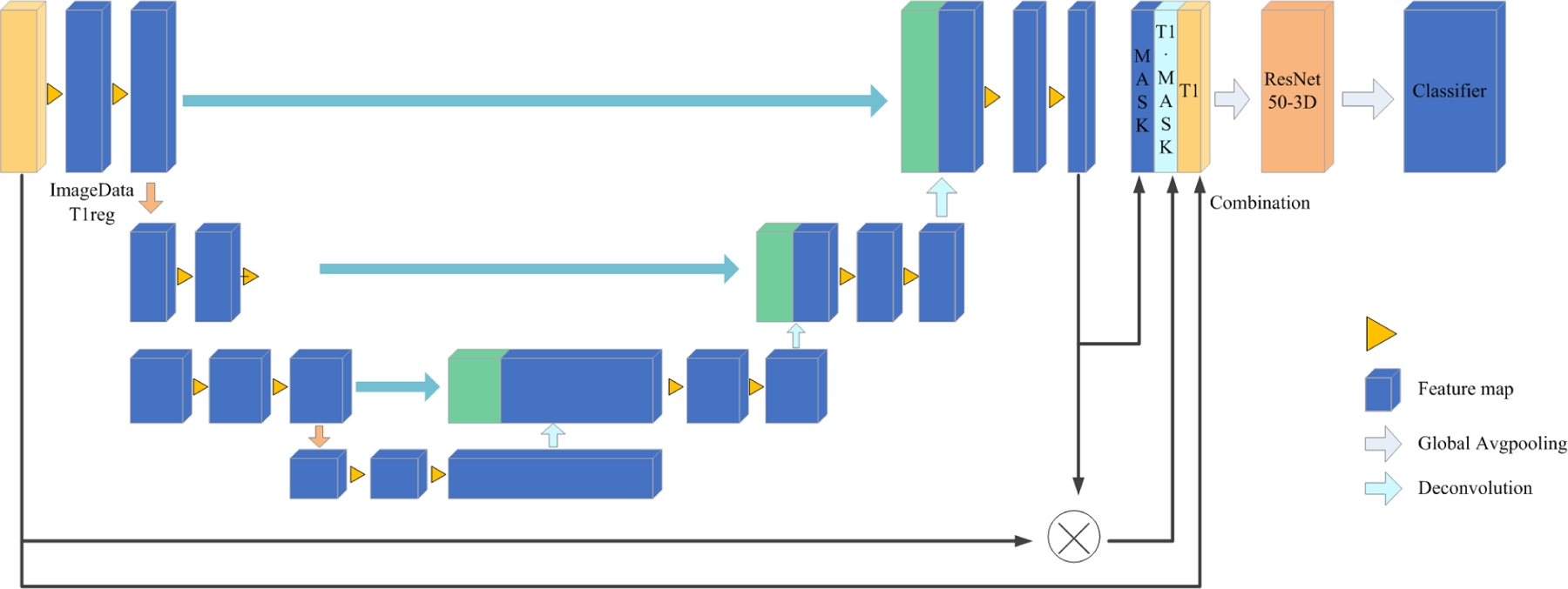
For segmentation, we used the 3D U-shaped CNN architecture shown in Fig.2. The inputs for the segmentation network are the original images and the predicted masks. The output is the segmented neurocranium.

Figure 2.

The main structure of the model is based on a 3D U-Net.¹⁵ First, the 256*256*256 pixel images were used as network inputs. This U-net, like the standard U-Net, has analysis and synthesis paths with four resolution steps each. Each layer in the analysis route has two 3*3*3 convolutions, a rectified linear unit (ReLu), a 2*2*2 max pooling with strides of two in each dimension, and finally a rectified linear unit (ReLu). Each layer in the synthesis route consists of two 3*3*3 convolutions followed by a ReLu, followed by an upconvolution of 2*2*2 by strides of two in each dimension. The necessary high resolution features for the synthesis path are provided via shortcut connections from layers of equal resolution in the analysis path. A 1*1*1 convolution in the final layer lowers the number of output channels to the number of labels, which in our instance is 2. We prevent bottlenecks by tripling the number of channels even before max pooling. This strategy is used in the synthesis path as well.

When predicting the neurocranium mask, we used the sliding window of 96 * 96 * 96 on the input data. In the prediction process, there were some incorrectly recognized voxels, which are scattered in the whole image space. Because the region of interest(ROI) generally exists continuously in the input data space, we used the maximum connected region algorithm¹⁹ to reduce the impact of noise points on the final recognition effect. At the same time, we found that there were discontinuous distributions in the head surface region in the prediction, resulting in holes in the recognition. We proposed a padding technique: For any two points ($x_1$, $y_1$) and ($x_2$, $y_2$), in each layer, if there is $\left(x_2-x_1+y_2-y_1+2\right)\le \theta$ — that is, the two points are within a certain threshold range $\theta$ — then find a connection path $r$, in which the coordinates connecting ($x_1$, $y_1$) and ($x_2$, $y_2$) are marked as ($I$, $J$). The optical path can be expressed by:

$$r_{opt}=min\left({\sum }_{i,j\in \left(I,J\right)}{r}_{i,j}-mas{k}_{i,j}\right)$$ (1)

where $mas{k}_{i,j}$ indicates a region that is currently recognized as a mask area.

2.3.2. Classification Network

For the classification network, we used ResNet²⁰ as the backbone and three different channels as input: the raw 3D image data, forecasted skull mask results, and results from multiplying the image by the skull mask elementwise. These three channels were combined to form the input of the next three channels, and finally, the classification model training between six categories (12, 18, 24, 36, 48, 60) months of age was carried out.

In order to investigate the interpretability of the classification model, the network was visualized by applying the Grad-CAM algorithm to produce a coarse localization map highlighting the important regions for classification. It uses the output probability to infer, in reverse, which region of the feature map has a strong correlation with the classification outcomes. The Grad-CAM heatmap is expressed by:

$$L_{Grad-CAM}=RELU\left({\sum }_k{w}_k{A}^k\right)$$ (2)

where $w_k$ is the class weights, $A^k$ is the corresponding feature maps, and the ReLU (rectified linear unit) function only permits the evaluation of positive attributes. Grad-CAM uses the gradient information of the last convolution layer flowing into the CNN to assign important values to each neuron. The last convolutional layer of the last Res-block was made transparent to the prediction of skull age so that we could analyze the differences in each skull region between different ages.

3. RESULTS

3.1. Segmentation Results

The segmentations were evaluated through the Dice similarity coefficient (Dice), which is usually used to calculate the similarity between two samples.

$$Dice\left(GT,Pred\right)=\frac{2are{a}_{GT}\cap are{a}_{Pred}}{are{a}_{GT}\cup are{a}_{Pred}}$$ (3)

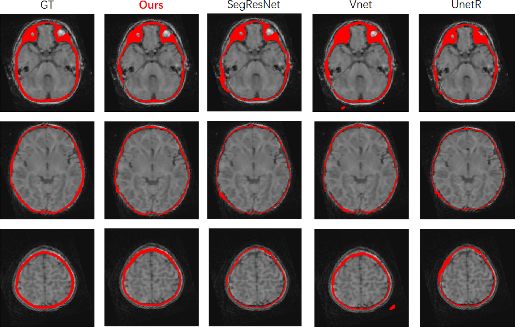
We compare the final effect of several common models, like Vnet,²¹ SegResNet,²² UnetR²³ in Table.2. We found that our NEC-NET produced higher Dice scores than other models and it is visually comparable with the ground truth, as shown in Fig.3.

Table 2.

Quantitative comparison of the performance of neurocranial segmentation models.

Model	NEC-NET	VNet	SegResNet	UNetR
Dice	0.8434	0.8171	0.8307	0.8025

Figure 3.

Qualitative comparison of segmentation results from different models.

3.2. Classification Results

The evaluation included 2 parts: the CNN models for image classification, and the heatmaps generated to interpret the CNNs.

When evaluating the classification model, we chose Top-1 Accuracy to evaluate the results and compared several common ResNet model structures in Table.3. In Top-1 Accuracy, the model prediction (the response with the highest probability) must precisely match the anticipated outcome. We found ResNet50–3D achieved higher classification accuracy.

Table 3.

Quantitative comparison of ACC performance of different ResNet model architectures.

Model	ResNet50-3D	ResNet101-3D	Resnet152-3D
ACC	0.7859	0.7309	0.7660

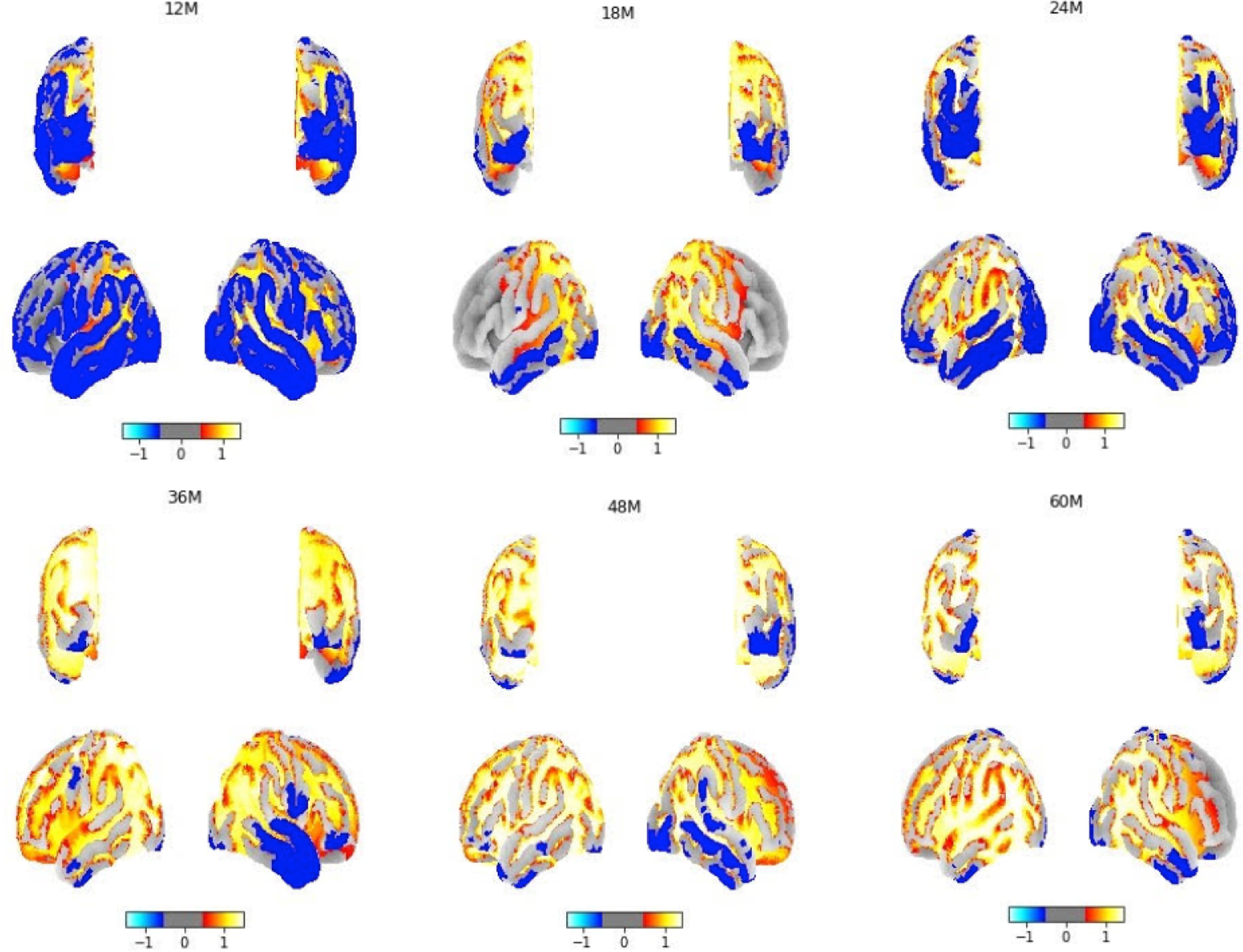
To verify that our Grad-CAM is meaningful at different ages, we calculated the 95th percentile threshold of the normalized neurocranium heatmaps and used an ANOVA test to perform statistical analysis between different age groups. All statistical analyses were performed in Python, with p < 0.01 as significance. Quantitative analysis of the heatmaps in Table.4 showed that the mean (±standard deviation) 95th percentile value of Grad-CAM was significantly different between age groups. Fig.4 shows the images generated using Grad-CAM based on trained classification models with different ages of subjects. The subsequent 3D plotting using volume rendering technologies with a template revealed that the most relevant voxels were distributed over the whole brain. The light color indicates the region has high significance and we found occipital bone and the temporal bone of the neurocranium are the areas that demonstrate high significance during brain development. This is reasonable because the skull sutures are situated in the posterior and occipital bone area and are known to allow for brain growth from birth to age two and frontal and temporal bones may continue to evolve even after age 2.

Table 4.

Mean (±standard deviation) 95th percentile value of Grad-CAM among age groups.

Age group	12m	18m	24m	36m	48m	60m	p value
95th percentile	0.2248±0.3235	0.8317±0.3136	1.1988±0.1308	1.2595±0.0908	1.2917±0.0439	1.1946±0.1039	< 0.01

Figure 4.

The projection of Grad-CAM neurocranial results to a brain template between 12–60 months of age, showing the regions that have discriminating features between ages.

4. DISCUSSION AND CONCLUSION

For the prevention and treatment of a variety of developmental disorders, especially premature suture fusion (also known as craniosynostosis), which results in skull deformities in about 0.05 percent of live births, it is crucial to understand the mechanisms underlying neurocranial development. In this work, we proposed a novel infant neurocranium development pipeline(NEC-NET). In our previous work, we characterized neurocranial thickness from MRI. Here we extend these results to produce the first-ever MRI-based maps of young children’s regional cranial shape development. This work also assessed the potential of several deep learning algorithms for neurocranium segmentation, and of the Grad-CAM approach for image classification using brain MRI data of infants. Our model’s segmentation performance produced a higher Dice value and is close to the ground truth, which shows our model is better than other ones and can reduce efforts from manual labeling. Also, the CNN model combined with Grad-CAM produced heatmaps for the classification task to indicate the significant regional differences across different age groups. The midline of the occipital lobe beneath the posterior fontanelle is where the neurocranium experiences the most significant change during early life. In future studies we plan to investigate younger age groups (3m,6m), and our model will help us to understand a more detailed timeline of neurocranial growth in health and disease.

REFERENCES

- [1].Li Z, Park B-K, Liu W, Zhang J, Reed MP, Rupp JD, Hoff CN, and Hu J, “A statistical skull geometry model for children 0–3 years old,” PloS one 10(5), e0127322 (2015). [DOI] [PMC free article] [PubMed] [Google Scholar]
- [2].Richtsmeier JT and Flaherty K, “Hand in glove: brain and skull in development and dysmorphogenesis,” Acta neuropathologica 125(4), 469–489 (2013). [DOI] [PMC free article] [PubMed] [Google Scholar]
- [3].Lillie EM, Urban JE, Lynch SK, Weaver AA, and Stitzel JD, “Evaluation of skull cortical thickness changes with age and sex from computed tomography scans,” Journal of bone and mineral research 31(2), 299–307 (2016). [DOI] [PubMed] [Google Scholar]
- [4].Bajwa M, Srinivasan D, Nishikawa H, Rodrigues D, Solanki G, and White N, “Normal fusion of the metopic suture,” Journal of Craniofacial Surgery 24(4), 1201–1205 (2013). [DOI] [PubMed] [Google Scholar]
- [5].Li G, Nie J, Wang L, Shi F, Lin W, Gilmore JH, and Shen D, “Mapping region-specific longitudinal cortical surface expansion from birth to 2 years of age,” Cerebral cortex 23(11), 2724–2733 (2013). [DOI] [PMC free article] [PubMed] [Google Scholar]
- [6].Li G, Nie J, Wang L, Shi F, Gilmore JH, Lin W, and Shen D, “Measuring the dynamic longitudinal cortex development in infants by reconstruction of temporally consistent cortical surfaces,” Neuroimage 90, 266–279 (2014). [DOI] [PMC free article] [PubMed] [Google Scholar]
- [7].Bastir M, Rosas A, and O’Higgins P, “Craniofacial levels and the morphological maturation of the human skull,” Journal of Anatomy 209(5), 637–654 (2006). [DOI] [PMC free article] [PubMed] [Google Scholar]
- [8].Gajawelli N, Deoni S, Shi J, Linguraru MG, Porras AR, Nelson MD, Tamrazi B, Rajagopalan V, Wang Y, and Lepore N, “Neurocranium thickness mapping in early childhood,” Scientific reports 10(1), 1–9 (2020). [DOI] [PMC free article] [PubMed] [Google Scholar]
- [9].Porras AR, Keating RF, Lee JS, and Linguraru MG, “Predictive statistical model of early cranial development,” IEEE Transactions on Biomedical Engineering 69(2), 537–546 (2021). [DOI] [PMC free article] [PubMed] [Google Scholar]
- [10].Gibson E, Giganti F, Hu Y, Bonmati E, Bandula S, Gurusamy K, Davidson B, Pereira SP, Clarkson MJ, and Barratt DC, “Automatic multi-organ segmentation on abdominal ct with dense v-networks,” IEEE transactions on medical imaging 37(8), 1822–1834 (2018). [DOI] [PMC free article] [PubMed] [Google Scholar]
- [11].Dolz J, Desrosiers C, and Ayed IB, “3d fully convolutional networks for subcortical segmentation in mri: A large-scale study,” NeuroImage 170, 456–470 (2018). [DOI] [PubMed] [Google Scholar]
- [12].Myronenko A, “3d mri brain tumor segmentation using autoencoder regularization,” in [International MICCAI Brainlesion Workshop], 311–320, Springer; (2018). [Google Scholar]
- [13].Zhu W, Huang Y, Zeng L, Chen X, Liu Y, Qian Z, Du N, Fan W, and Xie X, “Anatomynet: deep learning for fast and fully automated whole-volume segmentation of head and neck anatomy,” Medical physics 46(2), 576–589 (2019). [DOI] [PubMed] [Google Scholar]
- [14].Dalvit Carvalho da Silva R, Jenkyn TR, and Carranza VA, “Development of a convolutional neural network based skull segmentation in mri using standard tesselation language models,” Journal of Personalized Medicine 11(4), 310 (2021). [DOI] [PMC free article] [PubMed] [Google Scholar]
- [15].Çicek Ö, Abdulkadir A, Lienkamp SS, Brox T, and Ronneberger O, “3d u-net: learning dense volumetric segmentation from sparse annotation,” in [International conference on medical image computing and computer-assisted intervention], 424–432, Springer; (2016). [Google Scholar]
- [16].Rawat W and Wang Z, “Deep convolutional neural networks for image classification: A comprehensive review,” Neural computation 29(9), 2352–2449 (2017). [DOI] [PubMed] [Google Scholar]
- [17].Selvaraju RR, Cogswell M, Das A, Vedantam R, Parikh D, and Batra D, “Grad-cam: Visual explanations from deep networks via gradient-based localization,” in [Proceedings of the IEEE international conference on computer vision], 618–626 (2017). [Google Scholar]
- [18].Remer J, Croteau-Chonka E, Dean III DC, D’arpino S, Dirks H, Whiley D, and Deoni SC, “Quantifying cortical development in typically developing toddlers and young children, 1–6 years of age,” Neuroimage 153, 246–261 (2017). [DOI] [PMC free article] [PubMed] [Google Scholar]
- [19].King V, Rao S, and Tarjan R, “A faster deterministic maximum flow algorithm,” Journal of Algorithms 17(3), 447–474 (1994). [Google Scholar]
- [20].He K, Zhang X, Ren S, and Sun J, “Deep residual learning for image recognition,” in [Proceedings of the IEEE conference on computer vision and pattern recognition], 770–778 (2016). [Google Scholar]
- [21].Abdollahi A, Pradhan B, and Alamri A, “Vnet: An end-to-end fully convolutional neural network for road extraction from high-resolution remote sensing data,” IEEE Access 8, 179424–179436 (2020). [Google Scholar]
- [22].Chen X, Cheng G, Cai Y, Wen D, and Li H, “Semantic segmentation with modified deep residual networks,” in [Chinese Conference on Pattern Recognition], 42–54, Springer; (2016). [Google Scholar]
- [23].Hatamizadeh A, Tang Y, Nath V, Yang D, Myronenko A, Landman B, Roth HR, and Xu D, “Unetr: Transformers for 3d medical image segmentation,” in [Proceedings of the IEEE/CVF Winter Conference on Applications of Computer Vision], 574–584 (2022). [Google Scholar]