Nonnegative matrix factorization for analyzing state dependent neuronal network dynamics in calcium recordings

Abstract

Calcium imaging allows recording from hundreds of neurons in vivo with the ability to resolve single cell activity. Evaluating and analyzing neuronal responses, while also considering all dimensions of the data set to make specific conclusions, is extremely difficult. Often, descriptive statistics are used to analyze these forms of data. These analyses, however, remove variance by averaging the responses of single neurons across recording sessions, or across combinations of neurons, to create single quantitative metrics, losing the temporal dynamics of neuronal activity, and their responses relative to each other. Dimensionally Reduction (DR) methods serve as a good foundation for these analyses because they reduce the dimensions of the data into components, while still maintaining the variance. Nonnegative Matrix Factorization (NMF) is an especially promising DR analysis method for analyzing activity recorded in calcium imaging because of its mathematical constraints, which include positivity and linearity. We adapt NMF for our analyses and compare its performance to alternative dimensionality reduction methods on both artificial and in vivo data. We find that NMF is well-suited for analyzing calcium imaging recordings, accurately capturing the underlying dynamics of the data, and outperforming alternative methods in common use.

Introduction

Recent advances in neural recording methods have made it possible to collect large, complex data sets that can be used to study context-dependent neural dynamics in great detail^1,2. For example, calcium imaging allows simultaneous recording from hundreds of neurons in a single brain region in vivo, while maintaining single cell-resolution^3–7. Other tools allow cell “tagging” based on factors, including activity during a specified time window and molecular genotype^8–11. The resultant data set consists of several hundred time series thousands of points long, multiplicatively increasing per experimental condition added, in addition to any tagging data. The process of characterizing such single-cells responses, relating them to those of other cells across time, and accounting for the tagging information, all while considering changes in animal behavior, is a difficult but essential task.

Basic descriptive statistics (mean, median, variance) are a common approach to analyze large neural datasets. However, these approaches are limited because they average over the temporal dynamics of neuronal activity and can obscure interactions among neurons at fine time scales^12,13. Dimensionality reduction (DR) is a more sophisticated approach that can help to reveal low-dimensional dynamics by transforming high-dimensional data into interpretable, low-dimensional components¹⁴. Compressing the data in this way can preserve temporal patterns and correlations and focus subsequent analysis on the dynamical patterns of interest.

DR approaches have many applications in the analysis of neural data, including analysis of electrophysiological recordings^12,15,16, automation of trace extraction of neuronal activity in fluorescent recordings^1,17–25, and as a pre-processing step to more complex behavioral decoding²⁶. To analyze network dynamics in calcium recordings, non-linear DR methods have emerged to map dynamics to low dimensional manifolds^27–30. While excellent for very low dimensional visualization^31,32, the dynamics are difficult to interpret beyond the manifold being modeled, with manifolds being difficult to interpret beyond three dimensions. Further, dynamical non-linear methods have been applied to recover neural trajectories as a function of latent variables³³. Linear DR methods have likewise been employed to either statically cluster cells^21,34–36, or to abstractly analyze activity in low-dimensional subspaces^37–40.

While each methods have their own strengths as a function of different low dimensional representations, we aim to decompose our data into a lower dimensional series of neuronal sub-networks and their activities, to detect how neurons form flexible, correlated cell assemblies under different experimental contexts. We argue more generalized linear DR methods will provide a more interpretable representation of the data, at the cost of a few more dimensions than non-linear methods, dynamical or non-dynamical, as a function of having fewer tunable parameters and simpler mathematical decompositions. We further argue Nonnegative Matrix Factorization (NMF) is an especially promising linear decomposition method for analysis of activity recorded in calcium imaging in this context. NMF operates under the constraint that every element in the data, and the decomposition, be nonnegative⁴¹, as is naturally true for neuronal calcium traces²¹. Further, the positivity constraint, coupled with the linearity of the reduced dimensions, ensures that each of the dimensions sum to form a low dimensional representation of the data, simplifying the interpretation of the data⁴². In neuroscience, specifically in the context of calcium imaging, NMF has emerged as the state of the art method to estimate single neuron activity from fluorescent recordings^{17–19,22,24,25,43}, demonstrating efficacy signal de-mixing and functional imaging activity extraction²³. However for analyzing the dynamics of recorded neurons, it has been applied sparingly, either for quantifying single cell pairwise relationships⁴⁴ or statically clustering cells under a series of strict assumptions³⁵. Here, we develop an application of NMF to analyze holistic network activity (Fig. 1), comparing it to the most widely employed methods that provide a similar decomposition, capturing how precise sub-networks of neuronal dynamics evolve in different experimental contexts. To assess performance of the NMF approach, we generate artificial calcium imaging data from simulated ground-truth networks and assess how well our approach captures the underlying network structures responsible for the emergent dynamics of the network. We then apply the same NMF framework to characterize the dynamics of a representative in vivo calcium imaging data set. We conclude that, compared to alternative methods, NMF best captures the ground truth networks that underlie the observed calcium dynamics and provides a useful low-dimensional description of complex physiological data.

Fig. 1.

Representative Model Pipeline. (a) Recording Field of View (FOV) with Regions of Interest (ROIs). (b) Extracted fluorescent activity traces from ROIs. (c) Same recording FOV shown in (a) with ROIs colored according to largest component contribution. (d) Decomposed activities of the components shown in (c). (e) Sample truncated heatmap showing neuronal contribution or weight for each component.

Results

We test NMF against three existing DR approaches in common use: UMAP, PCA, and ICA. We do so using two different simulated neuronal network architectures to assess the relative performance of each DR approach, when the network structure is known. We first build a simple network with five groups of independent neurons, each with 20 neurons, in which the neurons in each independent node are perfectly connected (Fig. 2). In this architecture, a spike in one neuron in a node will drive all other neurons in that node to spike. We use such an architecture to test if, and how well, models can identify the five nodes given traces of simulated activity.

Fig. 2.

Nodal Network Architecture. (a) Diagram showing perfect intraconnection between neurons and independence between nodes. (b) Randomly selected calcium traces generated by the network. (c) Same randomly selected calcium traces shown in (b), but sorted according to node.

To further evaluate the performance between DR methods, we examine a more intricate network architecture aligned with our spontaneous calcium recordings. In doing so, we create five distinct random processes driving 150 neurons at varying degrees of strength (Fig. 3). This approach better reflects the dynamics we aim to capture, encompassing underlying activity patterns in diverse contexts driven by weighted sub-networks of neurons. Utilizing this surrogate architecture, our objective is to assess how effectively the models can extract both the underlying activity patterns, and the corresponding contributions by individual neurons, given a clear end target for performance assessment. We present two different analyses for both simulated network architectures. We both perform a qualitative analysis for a single generated network, and a more scaled quantitative approach for a series of 256 random instantiations and simulations of the networks. We find that NMF best captures the dynamics of the simulated networks, with components summing to provide an accurate macroscopic low dimensional representation of the data. We argue the parts-based representation provided inherently by NMF supports the improved performance for these data and the goal of interpretably extracting low dimensional neuronal network dynamics.

Fig. 3.

Artificial random propagating process network architecture. (a) Sample connection diagram showing all random processes projecting to all neurons. (b) Single histogram of generated connections between processes and neurons from sampled distribution.

Perfectly intraconnected, independent nodes

We generate the nodal networks and fit each of the DR methods to the simulated calcium traces. Initially, we evaluate the average variance explained and the Akaike Information Criterion (AIC) across 256 networks to gauge how well the models capture the original data at different lower dimensionality levels. Both NMF and PCA exhibit similar variance explanation patterns across all components, with the average variance explained stabilizing at five components (Fig. 4a, left axis), as required to capture the dynamics of simulated activity in five nodes. This stabilization is influenced by the introduction of unique noise increments in each trace (Eqs. 13, 14). Additionally, the AIC for the NMF method consistently minimizes at five components across all 256 model instantiations, effectively optimizing for the correct number of nodes (Fig. 4a, right axis). We note that the shape of the information criterion curve takes an inverse of the NMF variance explained curve until the inflection point, reflecting the inherent relationship between these two measures, arising from the AIC’s balance between model fit and complexity, contrasting with the NMF’s focus on maximizing explained variance.

Fig. 4.

Artificial Nodal Network Analysis. (a) Variance Explained for NMF and PCA, left axis (n = 256 networks) per component added to the model, and Akaike Information Criterion (AIC) for NMF, right axis (n = 256 networks). (b) Prediction visualization between nodes and components for single network. (c) Neuronal weights (y axis) for each model (panel) for each node (color) for each component (x axis). (d) Average between neurons inside and outside predicted nodes for each component (n = 256 networks). (e) Model assignment accuracy (n = 256 networks).

To evaluate how the different approaches capture the independent nodes of activity as components, we devised a discrete metric to determine success or failure of individual node assignment to components, detailed in the methods, for each architecture. We show the assignment success for a single model for each of the detailed DR methods (Fig. 4b). We find the best performance with the NMF method, which successfully maps each node to a component, followed by PCA, ICA, and UMAP. We repeat this process for 256 replicate models (Fig. 4e) and find that NMF always maps each node to a separate component, followed by PCA which performs with a mean accuracy of 0.8578, and then ICA and UMAP which perform with mean accuracies 0.6445 and 0.6242, respectively, and typically fail to successfully map the entire model.

We then visualize how each of the DR methods map the nodal patterns of activity to each of the components. We do so by showing the weight for each neuron, for each component, for each method, delimited by node (Fig. 4c), for a single instantiation of the simulated neural activity. In this example, we find a very clear separation of weights from each node for the NMF method; each component assigns weights to the neurons within a node. We argue this separation is a result of the parts-based representation that NMF inherently embodies⁴². In a parts-based representation, each component contributes an additive combination of components to faithfully represent the original data. This means that NMF decomposes the overall activity into identifiable parts, enabling a clear separation of weights for each node. Conversely, the PCA and ICA methods produce distributions of node weights with less clear separations within a component. While the first 5 components of the PCA method each identify neurons in each node, the constraints of the method result in counterbalancing variables that obfuscate the underlying input resulting in the data, hindering performance⁴⁵. UMAP poorly separates nodes into five components because a strength of UMAP, and manifold learning in general (e.g., TSNE), is visualization in very low dimensions (restricted to two or three dimensions)^31,32.

To provide a quantitative assessment of model performance, we calculate the average displacement between neuronal weights assigned to a component and all other weights within the same component, for all components of each of the 256 instantiations of the model (Fig. 4d). We do so to provide a quantitative and continuous measurement of model performance (separation between weights in node and not in node, at assigned component) beyond binary success/failure, with the magnitude indicating the degree of separation between the neurons in the assigned node and all other neurons within a given component. Normalized per model, a positive value describes an assigned node whose average weight was higher than the weights of the other node in that component. A negative value would then describe the opposite, with the magnitude of the displacement describing the degree of difference between the weights. Our findings reveal NMF best separates nodes into components, followed by PCA, UMAP, and ICA. While this supports our finding that NMF specifically assigns patterns of nodal activity to components, the other methods do tend to separate a majority of the nodes of neurons individually in each component (the normalized distance tends to exceed 0), with the differing representations being attributable to the different mathematical constraining during fitting (UMAP—very low dimensional manifold, PCA—orthogonality, ICA—independence). However, as we show in our next case, this structure breaks down on the introduction of more complicated data.

Random process propagation

We simulate a network with a more complicated architecture to further evaluate model performance. This architecture involves generating five underlying random processes to drive the network activity. Each underlying random process provides input to each of 150 neurons, with a weight randomly sampled from a generated exponential distribution (Fig. 3). By analyzing these artificial networks, we aim to probe how well NMF maps the random process by observations from the received neuronal inputs to components. We similarly aim to compare the performance and low dimensional representation of NMF and the other methods we implement.

Analyzing the average variance explained for all 256 uniquely seeded networks of this architecture, we find that NMF explains significantly more at all components (Fig. 5a, left axis). We argue this is a function of the difference between optimizations. Rather than having a strict orthogonality constraint between dimensions as in PCA, NMF aims to reconstruct the data with as little error as possible into the specified number of dimensions, allowing for explaining more variance with fewer components. The AIC shows a minimum at five components, the number of random processes used to generate the network (Fig. 5a, right axis), seeing a similar inverted relationship between AIC and variance explained.

Fig. 5.

Artificial Random Propagating Process Network Analysis. (a) Variance Explained for NMF and PCA, left axis (n = 256 networks) per component added to the model, and Akaike Information Criterion (AIC) for NMF, right axis (n = 256 networks). (b) Assignment visualization between nodes and components for single network. (c) Neuronal weights for NMF model (y axis) for each component (x axis) compared to assigned connection probabilities (color scale) for the predicted random process. (d) Correlation between neuronal weights for NMF model (y axis) and the respective assigned connection probability (x axis). (e) Average Correlation between neuronal weights for model and the respective assigned connection probabilities (n = 256 networks). (f) Model assignment accuracy (n = 256 networks). (g) Correlation between component activity from NMF model and assigned random process activity. (h) Correlations between component activity from model and assigned random process activity (n = 256 networks).

We quantify assignment success of this model differently from the nodal architecture, due to the more continuous nature of the data, detailed in the methods. For or an example model instantiation (Fig. 5b), only the NMF method successfully assigns each process to one component. Assessing the performance over 256 realizations of the network (Fig. 5f), we find that NMF successfully assigns each random process to a component. Consistent with the results for the nodal architecture, the other methods (PCA, ICA, and UMAP) have reduced performance. We conclude that NMF reconstructs the latent network structure from the observed data, capturing the five underlying random processes in a parts-based representation. Beyond discrete prediction, we consider the correlation between the assigned connection probabilities from the latent processes to the observed neurons, and the neuronal weights of the predicted component. To start, we visualize the results for one instance of the NMF model, relating the neuronal weights of each component to the assigned outgoing connection probability from the assigned underlying random process to each neuron (Fig. 5c). We find that large neuronal weights in each component tend to occur for large connection probabilities for the predicted random process with a high correlation of 0.84 (Fig. 5d). Repeating this analysis for 256 realizations of the model, and regardless of prediction success, we find that NMF consistently infers components with high correlations between the connection probabilities and weights (Fig. 5e), and is always able to successfully map all underlying processes to separate components (Fig. 5f). The other methods have reduced performance, consistent with the results for the nodal architecture with PCA, ICA, and UMAP following in performance, respectively.

We finally analyze how the activity of each component correlates with the activity of the underlying random process. Qualitatively, for a single realization of the model, the component activity captures the underlying processes very well (Fig. 5g) with correlations between the activities exceeding 0.85. Repeating this analysis across 256 realizations of the network, we once again find that NMF best captures the activity of the latent input processes, followed by PCA and ICA (Fig. 5h); we note that UMAP does not estimate the times series of the latent processes. To assess computational performance, we compare the median run time for the 256 models of this architecture. Because PCA is a well solved linear algebra problem (singular value decomposition of a matrix)⁴⁵, it is the shortest median run time of 0.0245 s. Of the three optimization methods, NMF and ICA have comparable median run times (0.7349 s and 0.7342 s, respectively. UMAP has the longest median run time of 1.4906 s, even after we exclude UMAP’s rather high overhead for initialization. This discrepancy can be attributed to model complexity (linearity of NMF and ICA, and non-linearity for UMAP).

We propose that the positivity and parts-based representation of the NMF method enable accurate reconstruct of the high-dimensional activity through low dimensional inputs. We propose that the constraints implemented by the PCA and ICA methods may obfuscate inputs to the observed neural network in its low dimensional representations. Finally, we interpret the poor performance of the UMAP method as indicating this method is better adapted for low dimensional visualization of less variant data. We conclude that NMF accurately reconstructs the latent inputs to a biophysically-motivated neuronal network that simulates calcium fluorescence recordings, despite multiple barriers to accurate identification (e.g., the underlying process is unobserved, with random connectivity to the observed neurons whose calcium signal is obfuscated with two types of noise). These results demonstrate NMF outperforms existing methods in common use to extract the underlying dynamics present in a series of neuronal activities recorded in calcium imaging.

Awake-state data

As a final proof of concept, we analyze application of the DR methods to awake state calcium imaging recordings from 36 mice. In doing so we apply the same analytical framework as for the simulated data. Analysis of the variance explained for each model (Fig. 6a) shows similar performance between the NMF and PCA methods, with a small but highly significant trend towards increased values for the NMF method (p < 10^− 6, Wilcoxon Signed-Rank test). This small advantage in increased variance explained may be due to the NMF method acting to capture the original data as quickly as possible into a set number of components (Eq. 2), rather than using a complex geometrical constraint to analyze the data⁴⁶. We further find that NMF, using AIC, identifies an optimal number of components to describe the data in each of the recordings (Fig. 6b), with number of neurons helping inform the number of components at a correlation of 0.662. We qualitatively characterize an NMF model fit to a single recording, using 18 components as determined by AIC. When characterizing the neuronal weights estimated by the NMF method, we find behavior consistent with the simulated random process network (Fig. 6c); the NMF method results in in the neuronal weights with an approximate exponential distribution (Fig. 6d), with most neurons contributing little to the overall network activity, and few neurons very significantly contributing. We further briefly characterize the correlations between the activity for each decomposed component (Fig. 6e), finding that pairwise correlations are consistently low between them (Fig. 6f). Given that the correlations are low, and we capture a significant portion of the variance, we interpret these results to indicate that NMF, and the parts-based nature of the model, successfully extracts unique predominant patterns of activity in the data. We conclude that, applied to these in vivo calcium imaging recordings, the NMF method identifies components with distinct (uncoupled) dynamics.

Fig. 6.

Baseline Awake State Network Analysis (a) Variance Explained for NMF and PCA, left axis (n = 36 mice) per component added to the model, and Akaike Information Criterion (AIC) for NMF, right axis (n = 36 mice). (b) Correlation between number of neurons (x axis) and number of optimized components (y axis) (n = 36 mice). (c) Neuronal weights for NMF model (y axis) for each component (x axis) for a single mouse. (d) Neuronal weight histogram from NMF model for the same mouse as (c). (e) Component activity for NMF model of the same mouse as in (c) and (d). (f) Pairwise correlations between component activities shown in (e)

We note the comparison between NMF and PCA for variance explained (Fig. 6a) is the only objective comparison possible here, because the in vivo dataset lacks ground truth, making further comparison between methods confusing and counterproductive.

While we demonstrate here that we successfully decompose statistically similar data from our simulations into statistically similar models, future work will relate inferred components and dynamics to experimentally elucidating biological mechanisms and behavior. We conclude that the NMF method is a promising tool to analyze neuronal network dynamics and identify meaningly sub-network activity via a relatively simple and interpretable approach.

Discussion

We have developed an analytical pipeline to more thoroughly model neuronal network dynamics with NMF, considering all information provided by the model in its low dimensional representation. We generate a series of calcium traces recorded from ground-truth artificial neuronal networks at two degrees of complexity to assess how well our analyses extract the ground-truth responsible for the simulated dynamics, and compare the performance of NMF to UMAP, PCA, and ICA. We find the NMF significantly performs the best, followed by PCA, ICA, and UMAP, respectively. We then apply our NMF pipeline to a series of in vivo baseline recordings and find that NMF confers a similar, and easily interpretable representation to the underlying random process network.

We argue this performance is a result of the “parts-based representation” conferred by NMF⁴². Because every single element of the model is necessarily positive, and the decomposition is aiming to recapture the original data, every component sums to give a low dimensional macroscopic representation of the original data. Interpreting the decomposition as the sum of its parts, rather than a complex cancelling of variables to achieve an algebraic constraint, as in PCA⁴⁵, results in NMF being able to provide a better representation of the dynamics. Further, the only fundamental assumption made in NMF is that the data can be represented exclusively as positive values. Our other methods require more stringent assumptions. UMAP makes the assumption that the data can be embedded on a low-dimensional manifold⁴⁷. While very advantageous in less variant data (large scale trial averaged electrophysiological recordings⁴⁸), we argue our data is far too variant with limited scalability (single trial, single recording) for this method to be as effective. ICA assumes that components are both non-normal, and independent⁴⁶. While the assumption of non-normality of traces, variables, is a positive feature given that calcium traces are clearly non-normal data, we argue it is unfair to assume sub-network dynamics are completely independent of each other. Finally, PCA assumes the data is best described by the eigenvectors of the covariance matrix⁴⁵. We note that this algebraic constraint does provide PCA the unique attribute of the model being the same for the first k components, regardless of the number of components fit. NMF, UMAP, AND ICA will differ in their representation of the data, dependent on the number of components fit to. As a result, PCA is guaranteed to perfectly lossless in an inverse transformation of the data, given all components. However, PCA is clearly less efficient than NMF in generating compact descriptions of data like ours.

As we mention in the introduction, a version of NMF, specifically Constrained Nonnegative Matrix Factorization (CNMF) has become nearly ubiquitous for automated trace extraction from calcium recordings^{1,17,18,20,25}, including a adaptions for microscopic endoscope data²². CNMF allows for the incorporation of constraints when there is a priori knowledge to build them. With our data, we have no a priori knowledge regarding connectivity, and we show that the unconstrained NMF method performs well. However, it would be feasible to modify our analytical pipeline to account for known constraints in other cases.

While clearly productive for analyzing local calcium recordings, NMF’s nonnegativity assumption makes it well-suited for potentially analyzing large-scale anatomical connectome data or functional imaging experiments (given the data were nonnegative). It can identify patterns of co-activation or synchronization among brain regions, revealing the modular organization of brain activity and interactions between assemblies. In the context of anatomical connectome mapping, NMF could uncover patterns of structural connectivity that give rise to modules in the brain. However, the structure in functional imaging and anatomical connectome data is complex and multifaceted. In specific analysis cases such as these constraining towards a particular solution (CNMF) could be advantageous.

Hierarchical clustering has also emerged as a prominent method to analyze these large scale data⁴⁹. While both hierarchical clustering and NMF aim to reveal underlying network structures, there are key differences between these approaches. Hierarchical clustering discretely assigns each neuron to single clusters based on activity similarity, while NMF reduce the data into components with each neuron having a weighted contribution to each component. This allows NMF to capture overlapping and graded membership of neurons in multiple sub-networks. Moreover, NMF’s parts-based nature provides a more interpretable representation compared to that of static clustering, which can be more difficult to interpret.

NMF’s performance is dependent on the statistical characteristics we outline above, and different DR methods may emphasize different aspects of the data structure dependent on their assumptions and the analysis objectives. For example, PCA identifies orthogonal components capturing maximum variance, while ICA identifies statistically independent sources. These methods may capture different facets of the brain’s functional and structural organization compared to NMF.

Similarly, inhibitory responses, where the fluorescence drops below the neuron’s baseline fluorescence, have been observed in calcium imaging⁵⁰. Here, where we focus on extracting the dominant patterns and underlying structure of the neuronal activity, the impact of these minor negative deviations in the fluorescence are statistically very minor. As a result, such minor effects can be lost amongst the other variability present in the activity, which can be captured by alternative statistical methods⁵⁰.

This pipeline was developed with the intent of analyzing state dependent neuronal network dynamics, and future work will analyze differential network dynamics that arise from unique experimental contexts. However, NMF, and other DR methods, require an underlying structure in the data and can be especially sensitive to potential extremes in the number of components and rates of activity in the network. An extreme sparsity or extreme saturation of events will lead to a much noisier representation in the model. Further, a fundamental assumption of DR is that the data can be represented with significantly fewer components than there are neurons¹². Data that would carry hundreds of underlying drivers of activity (or any case where the number of patterns approach the number of neurons) would be obfuscated in a model such as this. Deep learning, on the other hand, requires immense “ground truth” data sets for training. While deep learning models have recently emerged as an excellent tool for supervised learning, generally in neuroscience^51–54, and specifically for decoding behavioral events recorded with calcium imaging^26,55, in this case we are seeking to describe data with no such training set or “ground truth” available. Instead, we compare unsupervised methods to solve the specific problem of detecting reducing hundreds of neurons into components, or sub-networks, or cell assemblies.” Therefore, this approach will enable more sophisticated and nuanced unsupervised analysis of different states of neuronal networks, and how they shift as a function of context.

In sum, NMF provides a superior method for the holistic analysis of network dynamics recorded in calcium imaging. This analysis is able to go beyond summary statistics, providing a low dimensional representation of dynamics while still considering the activities of each neuron. The mathematical constraints required by NMF, linearity and positivity, complement the nature of fluorescent recording and neuronal activities well. Further, the parts-based nature of NMF provides a simple and interpretable representation of sub-networks of activity summing to drive macroscopic dynamics. As a result, we have developed an NMF pipeline to be an exceptionally valuable tool for elegantly demystifying shifting neuronal network dynamics.

Methods

Dimensionality reduction (DR) methods

Nonnegative matrix factorization (NMF)

NMF is a linear, matrix-decomposition method requiring all elements be nonnegative⁴¹. Each reduced dimension, or component, identified in NMF can be interpreted as a specific combination of input features representing distinct sources of variance in the data⁴². The components then sum to represent the original data, rather than canceling variables (using negativity) to achieve a geometrically strict representation⁴⁵. Mathematically, NMF decomposes an original matrix X into two constituent, lower rank, matrices W and H, given by:

1

with the aim of iteratively updating W and H to minimize an objective function so that the product of the two deconstructed matrices optimally reconstructs the original⁴¹. Here, X is a column-wise representation of the data, where each column is the time-series fluorescent activity of a neuron (Fig. 1b) extracted from the recording (Fig. 1a), that is decomposed into two lower rank matrices, W and H. For NMF, W can be interpreted as a feature matrix, each vector representing a distinct pattern in the input data, and H interpreted as a coefficient matrix, representing the contribution of each feature vector to each point in the original matrix. When using DR for analyses, especially in the context of neural recordings, the underlying assumption is that the original matrix can be decomposed into a lower rank series of matrices. The rank, k, should be significantly smaller than n (k < < n), the number of neurons recorded, while still recapturing a majority of the variance present in the data⁵⁶. Model performance can be assessed by the variance explained as represented by the coefficient of determination (R²)⁵⁷, given by:

2

where

3

4

Thus, the model captures the original data perfectly in the limit as R² approaches one. R² increases as components are added, because the rank of the two constituent matrices are increasing, capturing more variance. Akaike Information Criterion (AIC) has been adapted for NMF to inform the rank to which the dimensionality should be reduced^42,58, with the optimal model minimizing it⁵⁹; for our implementation of NMF:

5

Where R² is the reconstruction error defined in Eq. (2), σ² is the estimated variance of the data set, k is the number of components the model is decomposing into, n is the number of neurons in the recording, and t is the number of time points in each of the time series being decomposed. For our analysis, we interpret each row of H as a sub-network, with each entry of that row as a neuron’s contribution of to that sub-network (Fig. 1e). Each column of W is then interpreted as the time-series for that sub-network (Fig. 1d). Further, the neurons in the original recording FOV can be artificially reconstructed to provide visualization of sub-network contribution (Fig. 1c). We provide the pseudocode from an implementation of the NMF analysis pipeline: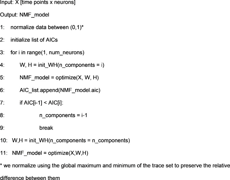

The above pipeline describes the sequence of using AIC to find an optimal number of components, and then fit a model to that number of components. Our implementation of NMF is a modification of the implementation found in Python’s Scikit-Learn package⁶⁰. We manually initialize W and H, as opposed to the automated method found in the package, due to the wide variety of initialization methods possible for NMF^61,62, and to maintain consistent, precise, and easily reproduceable control over the initial conditions of our models. For the analyses found in this paper, we apply nonnegative dual singular value decomposition (nndsvd), a consistent and efficient initialization method⁶³. Further, we implement variance explained and AIC for automatic model selection, as they are not part of the base implementation in the package.

Principal component analysis (PCA)

We implement PCA because of its widespread use in neural data analysis^{15,21,37–39,64–66}. PCA, efficiently calculated by a Singular Value Decomposition (SVD)⁴⁵:

6

where X is a column-wise representation of our data (i.e., each column is the time-series fluorescent activity of a neuron, assumed to have zero mean) decomposed into U, Σ, and V^T. V^T is the set of basis or singular vectors, also referred to as the principal components (PCs) of the original matrix, where each row of this matrix is a component of the data. Further, each of the PCs are necessarily orthogonal to each other by construction. U is the projection of the original matrix X onto the principal components in V^T, and Σ is a matrix containing the singular values of X describing the magnitude of the transformation, ordered by decreasing singular values⁴⁵. The variance explained by a PC is the proportion of its singular value compared to the sum of all singular values. For our analysis, we interpret each PC as a sub-network or prevalent pattern of activity, with each entry of the PC being a neuron’s weight or contribution to that PC. We then interpret the projection of the data onto each PC as the activity or time series of that sub-network, attributing the dominance of that sub-network to the variance explained. Our implementation of PCA is a modification of the implementation found in Python’s Scikit-Learn package⁶⁰. We provide the pseudocode from an implementation of the PCA pipeline below: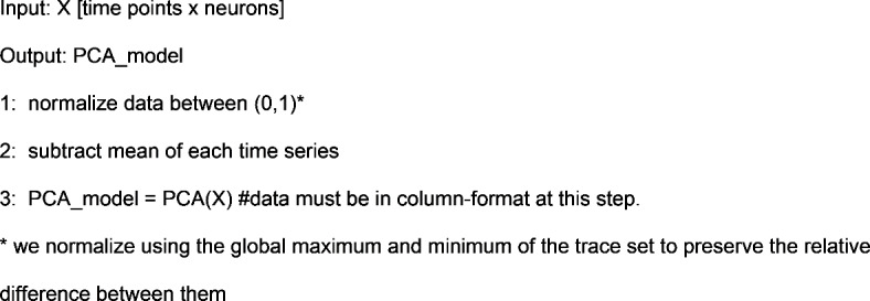

This is a modification of the implementation of PCA found in sklearn⁶⁰. PCA calls for every variable, or trace in our case, to be centered about zero⁴⁵. However, we remove the uniform normalization from sklearn’s implementation to allow for finer tuning of data normalization before decomposition with the model.

Independent component analysis (ICA)

We implement ICA because of its ability to extract independent sources from complex signals, which could help separate overlapping patterns of neural activity in a single calcium recording. While ICA has been used for automated trace extraction in calcium recordings⁶⁷, this approach has seen limited application in the further analyses of neural signals estimated calcium recordings. ICA is a statistical technique that aims to decompose a multivariate signal into statistically independent components⁴⁶, rather than a set of orthogonal components, as found in PCA. ICA operates under the assumption that k independent sources produce the data, and that the data are a linear mixture of these underlying sources. ICA assumes the data to be a linear mixture of sources:

7

where x is the original data, s are the underlying independent sources, and A is a mixing matrix that mixes the components of the sources⁴⁶.

In practice, the independent sources found in s, are decomposed using an unmixing matrix, W, such that the linear transformation of the data by W, estimates the underlying independent sources⁴⁶:

8

Given that W transforms x to estimate the independent sources, we interpret the components of W as the contribution of each neuron to the sub-network activities, which are the independent sources in s. Here, we interpret the s independent sources as the underlying patterns of activity of each sub-network that drive the observed dynamics. Like PCA, ICA assumes that inputs are zero mean. While PCA is designed to maximize the variance of the data along the principal components⁴⁵, ICA attempts to separate the data into k independent sources. We use the fastICA implementation found in sklearn⁶⁰, and provide the pseudocode from an implementation of the ICA analysis pipeline below:

While ICA calls for unit variance for each of the features, which in this case would be the calcium time series, we maintain the relative difference in variance between each neuronal time series to maintain the relative difference in activity recorded as a function of the fluorescence.

Uniform manifold-approximation projection (UMAP)

We implement UMAP because of its increasing use to analyze life science data^48,68 and its ability to capture non-linear relationships. UMAP has been shown to capture complex patterns to visualize and cluster data in very low dimensions⁴⁷, though the technique remains untested on calcium recordings. Briefly, UMAP aims to optimize between preserving local and global structures, where structure is local between neighboring points and global between data points extending beyond the neighborhood. In neuronal calcium imaging, “neighborhood” refers to local relationships among neurons with similar activity patterns at a time point, while global relationships extend beyond those neighbors at the same point. UMAP subsequently directly maps this structure to a lower dimension⁴⁷, resulting in the output being a single matrix (the equivalent of H, V^T, and S), and not a product of matrices. Therefore, UMAP does not provide temporal information about the activity of the lower dimensional patterns or sub-networks (Table 1). Further, there is no well-established way to quantify variance explained in UMAP as in the other linear methods. We use the python package UMAP-learn to implement UMAP, and provide the pseudocode from an implementation of the UMAP analysis pipeline below:

Table 1.

Model attributes.

Model	Variance explained	Information criterion	Neuronal weights	Decomposed activity
NMF	✓	✓	✓	✓
UMAP	X	X	✓	X
PCA	✓	X	✓	✓
ICA	X	X	✓	✓

In addition to the number of components, k, being a manually set hyperparameter, the number of points in the neighborhood is also manually set, in addition to the dozens of other tunable parameters in the package⁴⁷. Because our main objective is to identify how neurons group to form sub-networks and shift as a function of experimental contexts, we apply UMAP to decompose the data X into a k x n matrix. k is the number of components or subnetworks we determine to decompose into, while n is the number of neurons, aiming to give a similar representation to H, V^T, and S in our other methods.

Network simulation methods

To assess performance of the DR methods, we implement two simulation paradigms. In each paradigm, we simulate the spiking activity in a network of interconnected neurons and estimate calcium imaging traces for each neuron. We then apply each DR approach to the simulated calcium fluorescence data. We describe each simulation paradigm below.

Perfectly intraconnected, independent nodes

We first consider a network of 100 neurons organized into 5 independent nodes, each consisting of 20 neurons. Neurons within the same node are perfectly connected, such that a spike by any neuron in one node produces a spike in all other neurons in that node. Neurons in different nodes are disconnected, such that activity in two neurons of different nodes are independent (Fig. 2a). The activity of a single neuron is governed by a basic Poisson spike generator⁶⁹, given by:

9

where a neuron spikes at time t if x_rand (uniform [0, 1]) is less than the product of the set firing rate, r, and the time step, dt. We update this generator to include additional network effects, and a refractory period. We represent the connectivity between neurons as an adjacency matrix A. Within any node of 20 neurons, A is 1, while between nodes A is 0; we exclude self-connections by setting the diagonal of A to 0. We also include a refractory period of duration q time steps, such that after a spike a neuron is temporarily unable to generate a subsequent spike.

We simulate the spiking activity of a single neuron in this network n = {1,2, … N} as:

10

where r = 3 is the set nominal rate, N = 100 is the total number of neurons, k = 5 is the number of nodes, and dt is the time step. A is the adjacency matrix of dimensions N x N, where each row represents the incoming connections to a neuron, and each column represents the outgoing connections of a neuron, and is the refractory state of neuron n at time t. A neuron spikes at time t if the randomly generated number (uniform [0,1]) is less than the product in Eq. (10). We note that any multiplication of an adjacency of 1 to neuron n, in conjunction with a spike at time t-1 will result in a spike at time t in neuron n, given the neuron n is not in a refractory state. After simulating the network we convolve each spike train with a calcium kernel^35,70 as described below. The result is a series of 100 fluorescent neuronal activities (Fig. 2b), of which there are five groups of twenty that are perfectly correlated (Fig. 2c).

Random process propagation

We generate a second simulation paradigm to more closely represent a physiologically relevant dynamic in calcium fluorescence data: a small number of independent random spiking patterns simultaneously driving calcium events in all neurons. To do so, we first simulate k = 5 independent spiking patterns as,

11

We then consider a population of N = 150 neurons that receive inputs from each of the underlying spiking patters (Fig. 3a) weighted as follow: 20% of the neurons have weights uniformly distributed between 0.2 and 1.0, and 80% of the neurons have weights exponentially distributed (rate parameter ) with maximum value of 0.2 (Fig. 3b). In this way, most neurons are connected with weights following an exponential distribution⁷¹, and the few neurons with strong weights drive a majority of the activity. The resulting adjacency matrix A between the k spiking patterns and N neurons has dimensions k x N, where each element describes the weight of the kth underlying process input to neuron n = {1, 2, … N}. We simulate each neuron’s spike train as:

12

where n indicates the nth neuron, k indicates the kth underlying spike processes, and we include a refractory period for each neuron. Doing so results in N = 150 neuronal spike trains. We convolve the spike train of each neuron with the calcium kernel^35,70, resulting in simulated calcium data similar to our in vivo recordings, mirroring: activity rate, activity distribution, underlying macroscopic drivers, and calcium neuronal time series characteristics.

Calcium kernel

We convolve the simulated spike trains with the following calcium kernel to represent the fluorescence recorded from the genetically encoded calcium (GECI) kernel jGCaMP7f:

13

where Ca^+ 2_{t, t−1,b} are the calcium concentrations at t, t-1, and the baseline, respectively. Here, dt is the time step, is the time constant of the GECI, σ_c is the variance of the calcium noise, and _t is a random variable following the standard gaussian distribution. We then calculate the fluorescence as:

14

where F_t is the fluorescence at time t, α is the intensity, is the bias, σ_F is the variance of the calcium noise, and _t is a random variable following the standard gaussian distribution. We set to 0.265 and σ_c to 0.5 to match the kinetics of jGCaMP7f⁷². We set the calcium baseline to 0.1, A and α to 5, β to 10, and σ_F to 1³⁵.

Component assignment success

Perfectly intraconnected, indpendent nodes

To assess whether nodes were successfully assigned to components, we develop a framework for each of our generated network architectures. For the nodal model, we begin by summing the weights for each node, in each of the decomposed components, described by the pseudocode below:

The result is a five by five matrix, where the element [ i, j ] is the sum of the weights for neurons in the ith node for the jth component. To then determine success of prediction, we establish two conditions that must be met. First, within a particular component, the sum of weights for the node with the highest value should exceed the sums of weights for all other nodes within the same component. Second, this highest sum should also be the greatest for the node, across all components. By applying these conditions, we can assess the assignment for each node individually. In essence, once we obtain the aggregated weight matrix, an ideal model would exhibit the same element as the maximum value for each row and column.

Random process propagation

We calculate a 5 × 5 correlation matrix between the weights in each of the 5 components and the connection probabilities from each of the 5 generated random processes sampled from the defined exponential distribution. To assess assignment, we again consider two conditions. First, for a chosen component, the highest correlation with the connection probabilities from one random process should surpass the correlation to the other random processes in the same component. Second, this highest correlation within each component should identify a different random process; i.e., each component should identify a unique random process. We consider a component successfully assigned to one of the five random processes if its highest correlation is more correlated with that process than the other four processes.

Awake-state data

To investigate the application of each DR technique to in vivo recordings, we also consider calcium imaging data recorded from 36 awake mice. Briefly, recordings in layer 2/3 of murine S1 ¹³ were collected during the awake, resting state¹¹. Traces representing calcium transients were extracted from the recordings and processed using standard techniques⁷³.

Author contributions

Conceptualization, all authors; Methodology, DC; Validation, DC; Formal Analysis, DC; Investigation, DC; Resources, DC and JN; Software, DC; Data Curation, DC and JN; Writing—Original Draft, DC; Writing—Review and Editing, all authors; Visualization, DC; Supervision, JN, MAK, and JAW; Project Administration, DC; Funding Acquisition, DC and JAW.

Funding

Research reported in this publication was supported by the National Institute Of Mental Health of the National Institutes of Health (F31MH133306 to DC, R01MH085074 to JW). The content is solely the responsibility of the authors and does not necessarily represent the official views of the National Institutes of Health. Further, this research was partially supported by NIH Translational Research in Biomaterials Training Grant: T32 EB006359.

Data availability

Code to simulate synthetic neuronal networks is available in python, and all statistics of all models fit to the simulated neuronal networks are available in python .pkl format (Figs. 4 and 5). The extracted activity of the 36 awake baseline recordings, and all optimum models fit to them are further available in python .pkl format (Fig. 6). All materials can be requested by contacting the corresponding author, John A. White, and will be shared in their entirety upon request.

Declarations

Competing interests

The authors declare no competing interests.

References

- 1.Pnevmatikakis, E. A. Analysis pipelines for calcium imaging data. Curr. Opin. Neurobiol.55, 15–21 (2019). [DOI] [PubMed] [Google Scholar]
- 2.Stevenson, I. H. & Kording, K. P. How advances in neural recording affect data analysis. Nat. Neurosci.14, 139–142 (2011). [DOI] [PMC free article] [PubMed] [Google Scholar]
- 3.Stringer, C. & Pachitariu, M. Computational processing of neural recordings from calcium imaging data. Curr. Opin. Neurobiol.55, 22–31 (2019). [DOI] [PubMed] [Google Scholar]
- 4.Birkner, A., Tischbirek, C. H. & Konnerth, A. Improved deep two-photon calcium imaging in vivo. Cell Calcium64, 29–35 (2017). [DOI] [PubMed] [Google Scholar]
- 5.Chen, T.-W. et al. Ultrasensitive fluorescent proteins for imaging neuronal activity. Nature499, 295–300 (2013). [DOI] [PMC free article] [PubMed] [Google Scholar]
- 6.Zhang, Y. et al. Fast and sensitive GCaMP calcium indicators for imaging neural populations. Nature615, 884–891 (2023). [DOI] [PMC free article] [PubMed] [Google Scholar]
- 7.Ouzounov, D. G. et al. In vivo three-photon imaging of activity of GcamP6-labeled neurons deep in intact mouse brain. Nat. Methods14, 388–390 (2017). [DOI] [PMC free article] [PubMed] [Google Scholar]
- 8.Tonegawa, S., Liu, X., Ramirez, S. & Redondo, R. Memory engram cells have come of age. Neuron87, 918–931 (2015). [DOI] [PubMed] [Google Scholar]
- 9.Josselyn, S. A. & Tonegawa, S. Memory engrams: Recalling the past and imagining the future. Science367, (2020). [DOI] [PMC free article] [PubMed]
- 10.Kitamura, T. et al. Engrams and circuits crucial for systems consolidation of a memory. Science78, 73–78 (2017). [DOI] [PMC free article] [PubMed] [Google Scholar]
- 11.Norman, J. F., Rahsepar, B., Noueihed, J. & White, J. A. Determining the optimal expression method for dual-color imaging. J. Neurosci. Methods351, 109064 (2021). [DOI] [PMC free article] [PubMed] [Google Scholar]
- 12.Cunningham, J. P. & Yu, B. M. Dimensionality reduction for large-scale neural recordings. Nat. Neurosci.17, 1500–1509 (2014). [DOI] [PMC free article] [PubMed] [Google Scholar]
- 13.Sanger, T. D. & Kalaska, J. F. Crouching tiger, hidden dimensions. Nat. Neurosci.17, 338–340 (2014). [DOI] [PubMed] [Google Scholar]
- 14.Géron, A. Hands-on Machine Learning with Scikit-Learn, Keras, and TensorFlow: Concepts, Tools, and Techniques to Build Intelligent Systems. (O’Reilly Media, Inc, 2019).
- 15.Peyrache, A., Benchenane, K., Khamassi, M., Wiener, S. I. & Battaglia, F. P. Principal component analysis of ensemble recordings reveals cell assemblies at high temporal resolution. J. Comput. Neurosci.29, 309–325 (2010). [DOI] [PMC free article] [PubMed] [Google Scholar]
- 16.Low, R. J., Lewallen, S., Aronov, D., Nevers, R. & Tank, D. W. Probing Variability in a Cognitive Map Using Manifold Inference from Neural Dynamics. 10.1101/418939 (2018)
- 17.Giovannucci, A. et al. CaImAn an open source tool for scalable calcium imaging data analysis. eLife8, e38173 (2019). [DOI] [PMC free article] [PubMed] [Google Scholar]
- 18.Pnevmatikakis, E. A. et al. Simultaneous denoising, deconvolution, and demixing of calcium imaging data. Neuron89, 285–299 (2016). [DOI] [PMC free article] [PubMed] [Google Scholar]
- 19.Pachitariu, M. et al. Suite2p: Beyond 10,000 Neurons with Standard Two-Photon Microscopy. 10.1101/061507 (2016)
- 20.Pnevmatikakis, E. A. & Giovannucci, A. NoRMCorre: An online algorithm for piecewise rigid motion correction of calcium imaging data. J. Neurosci. Methods291, 83–94 (2017). [DOI] [PubMed] [Google Scholar]
- 21.Romano, S. A. et al. An integrated calcium imaging processing toolbox for the analysis of neuronal population dynamics. PLOS Comput. Biol.13, e1005526 (2017). [DOI] [PMC free article] [PubMed] [Google Scholar]
- 22.Zhou, P. et al. Efficient and accurate extraction of in vivo calcium signals from microendoscopic video data. eLife7, e28728 (2018). [DOI] [PMC free article] [PubMed] [Google Scholar]
- 23.Saxena, S. et al. Localized semi-nonnegative matrix factorization (LocaNMF) of widefield calcium imaging data. PLOS Comput. Biol.16, e1007791 (2020). [DOI] [PMC free article] [PubMed] [Google Scholar]
- 24.Bao, Y., Redington, E., Agarwal, A. & Gong, Y. Decontaminate traces from fluorescence calcium imaging videos using targeted non-negative matrix factorization. Front. Neurosci.15, 797421 (2022). [DOI] [PMC free article] [PubMed] [Google Scholar]
- 25.Zhuang, P. & Wu, J. Reinforcing Neuron Extraction from Calcium Imaging Data via Depth-Estimation Constrained Nonnegative Matrix Factorization. In 2022 IEEE International Conference on Image Processing (ICIP) 216–220 (IEEE, Bordeaux, 2022). 10.1109/ICIP46576.2022.9897521.
- 26.Batty, E. et al. BehaveNet: Nonlinear embedding and Bayesian neural decoding of behavioral videos. 12.
- 27.Sotskov, V. P., Pospelov, N. A., Plusnin, V. V. & Anokhin, K. V. Calcium imaging reveals fast tuning dynamics of hippocampal place cells and CA1 population activity during free exploration task in mice. Int. J. Mol. Sci.23, 638 (2022). [DOI] [PMC free article] [PubMed] [Google Scholar]
- 28.Rubin, A. et al. Revealing neural correlates of behavior without behavioral measurements. Nat. Commun.10, 4745 (2019). [DOI] [PMC free article] [PubMed] [Google Scholar]
- 29.Driscoll, L. N., Pettit, N. L., Minderer, M., Chettih, S. N. & Harvey, C. D. Dynamic reorganization of neuronal activity patterns in parietal cortex. Cell170, 986-999.e16 (2017). [DOI] [PMC free article] [PubMed] [Google Scholar]
- 30.Wenzel, M. et al. Reduced repertoire of cortical microstates and neuronal ensembles in medically induced loss of consciousness. Cell Syst.8, 467-474.e4 (2019). [DOI] [PMC free article] [PubMed] [Google Scholar]
- 31.Anowar, F., Sadaoui, S. & Selim, B. Conceptual and empirical comparison of dimensionality reduction algorithms (PCA, KPCA, LDA, MDS, SVD, LLE, ISOMAP, LE, ICA, t-SNE). Comput. Sci. Rev.40, 100378 (2021). [Google Scholar]
- 32.Izenman, A. J. Introduction to manifold learning: Introduction to manifold learning. Wiley Interdiscip. Rev. Comput. Stat.4, 439–446 (2012). [Google Scholar]
- 33.Koh, T. H. et al. Dimensionality reduction of calcium-imaged neuronal population activity. Nat. Comput. Sci.3, 71–85 (2022). [DOI] [PMC free article] [PubMed] [Google Scholar]
- 34.Ghandour, K. et al. Orchestrated ensemble activities constitute a hippocampal memory engram. Nat. Commun.10, 2637 (2019). [DOI] [PMC free article] [PubMed] [Google Scholar]
- 35.Nagayama, M. et al. Detecting cell assemblies by NMF-based clustering from calcium imaging data. Neural Netw.149, 29–39 (2022). [DOI] [PubMed] [Google Scholar]
- 36.Nagayama, M. et al. Sleep state analysis using calcium imaging data by non-negative matrix factorization. In Artificial Neural Networks and Machine Learning—ICANN 2019: Theoretical Neural Computation Vol. 11727 (eds Tetko, I. V. et al.) 102–113 (Springer, 2019). [Google Scholar]
- 37.Briggman, K. L., Abarbanel, H. D. I. & Kristan, W. B. Optical imaging of neuronal populations during decision-making. Science307, 896–901 (2005). [DOI] [PubMed] [Google Scholar]
- 38.Ahrens, M. B. et al. Brain-wide neuronal dynamics during motor adaptation in zebrafish. Nature485, 471–477 (2012). [DOI] [PMC free article] [PubMed] [Google Scholar]
- 39.Morcos, A. S. & Harvey, C. D. History-dependent variability in population dynamics during evidence accumulation in cortex. Nat. Neurosci.19, 1672–1681 (2016). [DOI] [PMC free article] [PubMed] [Google Scholar]
- 40.Makino, H. et al. Transformation of cortex-wide emergent properties during motor learning. Neuron94, 880-890.e8 (2017). [DOI] [PMC free article] [PubMed] [Google Scholar]
- 41.Lee, D. D. & Seung, H. S. Learning the parts of objects by non-negative matrix factorization. Nature401, 788–791 (1999). [DOI] [PubMed] [Google Scholar]
- 42.Devarajan, K. Nonnegative matrix factorization: An analytical and interpretive tool in computational biology. PLoS Comput. Biol.4, 12 (2008). [DOI] [PMC free article] [PubMed] [Google Scholar]
- 43.Sheintuch, L. et al. Tracking the same neurons across multiple days in Ca2+ imaging data. Cell Rep.21, 1102–1115 (2017). [DOI] [PMC free article] [PubMed] [Google Scholar]
- 44.Miyazaki, T. et al. Dynamics of cortical local connectivity during sleep-wake states and the homeostatic process. Cereb. Cortex30, 3977–3990 (2020). [DOI] [PubMed] [Google Scholar]
- 45.Shlens, J. A tutorial on principal component analysis. http://arxiv.org/abs/1404.1100 (2014).
- 46.Shlens, J. A tutorial on independent component analysis. http://arxiv.org/abs/1404.2986 (2014).
- 47.McInnes, L., Healy, J. & Melville, J. UMAP: Uniform manifold approximation and projection for dimension reduction. http://arxiv.org/abs/1802.03426 (2020).
- 48.Lee, E. K. et al. Non-linear dimensionality reduction on extracellular waveforms reveals cell type diversity in premotor cortex. eLife10, e67490 (2021). [DOI] [PMC free article] [PubMed] [Google Scholar]
- 49.Pacheco, D. A., Thiberge, S. Y., Pnevmatikakis, E. & Murthy, M. Auditory activity is diverse and widespread throughout the central brain of Drosophila. Nat. Neurosci.24, 93–104 (2021). [DOI] [PMC free article] [PubMed] [Google Scholar]
- 50.Vanwalleghem, G., Constantin, L. & Scott, E. K. Calcium imaging and the curse of negativity. Front. Neural Circuits14, 607391 (2021). [DOI] [PMC free article] [PubMed] [Google Scholar]
- 51.Kell, A. J. E., Yamins, D. L. K., Shook, E. N., Norman-Haignere, S. V. & McDermott, J. H. A task-optimized neural network replicates human auditory behavior, predicts brain responses, and reveals a cortical processing hierarchy. Neuron98, 630-644.e16 (2018). [DOI] [PubMed] [Google Scholar]
- 52.Nadalin, J. K. et al. Application of a convolutional neural network for fully-automated detection of spike ripples in the scalp electroencephalogram. J. Neurosci. Methods360, 109239 (2021). [DOI] [PMC free article] [PubMed] [Google Scholar]
- 53.Schlafly, E. D., Carbonero, D., Chu, C. J. & Kramer, M. A. A data augmentation procedure to improve detection of spike ripples in brain voltage recordings. Neurosci. Res.10.1016/j.neures.2024.07.005 (2024). [DOI] [PMC free article] [PubMed] [Google Scholar]
- 54.Richards, B. A. et al. A deep learning framework for neuroscience. Nat. Neurosci.22, 1761–1770 (2019). [DOI] [PMC free article] [PubMed] [Google Scholar]
- 55.Zhu, F. et al. A deep learning framework for inference of single-trial neural population dynamics from calcium imaging with subframe temporal resolution. Nat. Neurosci.25, 1724–1734 (2022). [DOI] [PMC free article] [PubMed] [Google Scholar]
- 56.Cunningham, J. P. & Ghahramani, Z. Linear dimensionality reduction: Survey, insights, and generalizations. 42.
- 57.Roh, J., Cheung, V. C. K. & Bizzi, E. Modules in the brain stem and spinal cord underlying motor behaviors. J. Neurophysiol.106, 1363–1378 (2011). [DOI] [PMC free article] [PubMed] [Google Scholar]
- 58.Cheung, V. C. K., Devarajan, K., Severini, G., Turolla, A. & Bonato, P. Decomposing time series data by a non-negative matrix factorization algorithm with temporally constrained coefficients. In 2015 37th Annual International Conference of the IEEE Engineering in Medicine and Biology Society (EMBC) 3496–3499 (IEEE, Milan, 2015). 10.1109/EMBC.2015.7319146. [DOI] [PMC free article] [PubMed]
- 59.Akaike, H. Information theory and an extension of the maximum likelihood principle. In Selected Papers of Hirotugu Akaike (eds Parzen, E. et al.) 199–213 (Springer, 1998). 10.1007/978-1-4612-1694-0_15. [Google Scholar]
- 60.Pedregosa, F. et al. Scikit-learn: Machine learning in python. J. Mach. Learn. Res. 6.
- 61.Esposito, F. A review on initialization methods for nonnegative matrix factorization: Towards omics data experiments. Mathematics9, 1006 (2021). [Google Scholar]
- 62.Hafshejani, S. F. & Moaberfard, Z. Initialization for nonnegative matrix factorization: A comprehensive review. http://arxiv.org/abs/2109.03874 (2021).
- 63.Boutsidis, C. & Gallopoulos, E. SVD based initialization: A head start for nonnegative matrix factorization. Pattern Recognit.41, 1350–1362 (2008). [Google Scholar]
- 64.Harvey, C. D., Coen, P. & Tank, D. W. Choice-specific sequences in parietal cortex during a virtual-navigation decision task. Nature484, 62–68 (2012). [DOI] [PMC free article] [PubMed] [Google Scholar]
- 65.Kato, H. K., Chu, M. W., Isaacson, J. S. & Komiyama, T. Dynamic sensory representations in the olfactory bulb: Modulation by wakefulness and experience. Neuron76, 962–975 (2012). [DOI] [PMC free article] [PubMed] [Google Scholar]
- 66.Awal, M. R., Wirak, G. S., Gabel, C. V. & Connor, C. W. Collapse of global neuronal states in Caenorhabditis elegans under isoflurane anesthesia. Anesthesiology133, 133–144 (2020). [DOI] [PMC free article] [PubMed] [Google Scholar]
- 67.Mukamel, E. A., Nimmerjahn, A. & Schnitzer, M. J. Automated analysis of cellular signals from large-scale calcium imaging data. Neuron63, 747–760 (2009). [DOI] [PMC free article] [PubMed] [Google Scholar]
- 68.Cid, E. et al. Sublayer- and cell-type-specific neurodegenerative transcriptional trajectories in hippocampal sclerosis. Cell Rep.35, 109229 (2021). [DOI] [PubMed] [Google Scholar]
- 69.Dayan, P., Abbott, L. F. & Abbott, L. F. Theoretical neuroscience: Computational and mathematical modeling of neural systems (MIT Press, 2005). [Google Scholar]
- 70.Vogelstein, J. T. et al. Spike inference from calcium imaging using sequential Monte Carlo methods. Biophys. J.97, 636–655 (2009). [DOI] [PMC free article] [PubMed] [Google Scholar]
- 71.Song, S., Sjöström, P. J., Reigl, M., Nelson, S. & Chklovskii, D. B. Highly nonrandom features of synaptic connectivity in local cortical circuits. PLoS Biol.3, e68 (2005). [DOI] [PMC free article] [PubMed] [Google Scholar]
- 72.Dana, H. et al. High-performance calcium sensors for imaging activity in neuronal populations and microcompartments. Nat. Methods16, 649–657 (2019). [DOI] [PubMed] [Google Scholar]
- 73.Noueihed, J. Unsupervised tracking and automated analysis of multi-population neural activity under anesthesia. (Boston University).
Associated Data
This section collects any data citations, data availability statements, or supplementary materials included in this article.
Data Availability Statement