Towards faster and robust solution for dynamic LR and QR factorization

Abstract

Dynamic LR and QR factorization are fundamental problems that exist widely in the control field. However, the existing solutions under noises are lack of convergence speed and anti-noise ability. To this end, this paper incorporates the advantages of Dynamic-Coefficient Type (DCT) and Integration-Enhance Type (IET) Zeroing Neural Dynamic (ZND), and proposes an Adaptive and Robust-Enhanced Neural Dynamic (AREND). On this basis, a Strategy of Integration-Coupling (SIC) is proposed to address multiple error function problems, improving model stability and application scenarios. This strategy is experimentally proven to be effective and has potential expansion capability. After that, the convergence and robustness of our AREND is theoretically analyzed. Furthermore, the proposed AREND is verified by numerical experiments of low-to-high dimensional factorization in comparison with existing solutions. Finally, the real-time 3-D Angle of Arrival (AoA) localization in multiple high-noise conditions, is validated to the accuracy of the proposed model. Code is available at https://github.com/Alana2a3/AREND-Code-Implementation.

Introduction

Matrix factorization is a fundamental tool to simplify problems by splitting a matrix into the form of a product of several matrices of a particular type^1–4. Among them, LR and QR factorization, as the names suggest: are a matrix M factorization into two matrices. The LR factorization is: a unit lower triangular matrix $\mathrm{\Lambda }$ and an upper triangular matrix $R_L$ to the multiplication, and the QR factorization is: an orthogonal matrix Q and an upper triangular matrix $R_Q$ to the multiplication. The LR factorization can be utilized in parallel computation^5–7, applied in many engineering and technology needs like data movement analysis and circuit simulation^8–10. Due to the special attributes of the orthogonal matrix after the QR factorization, the computation is more efficient and stable, often applied in least squares problems and optimization problems^11,12. In real life, QR factorization is applied in areas such as the smart grid, pathological matrix problems, and harmonic compensation of inductors, among others^13–16.

In practical applications, matrix factorization has to account for noise in the environment. To improve the stability of matrix factorization, algorithms minimize the accumulation and amplification of noise in the computation to provide reliable results^17–22. With the development of neural dynamics in various fields^23–30, researchers turn their attention to matrix factorization. Most of the work is on static matrices. While for the general case of dynamic matrices, ^31,32only assume quasi-stationary case, and ^33,34have no consideration of noise conditions. ³⁵more focuses on improving the convergence speed of the solution. But under the noisy condition, it is more disturbing to the factorization. The practical solution for factorization is not satisfactory.

In recent years, a novel kind of neural dynamic called Zeroing Neural Dynamic (ZND) has been proposed³⁶, which is commonly employed for solving dynamic problems. ZNDs utilize first-order derivative and are susceptible to noise. In order to improve the accuracy of ZNDs, they are extended to solve for a variety of noise types, resulting in an Integration-Enhance Type (IET) of ZNDs, which have been designed by control theory³⁷, applied to robotic arm³⁸, and used for constrained dynamic optimization³⁹, among other applications. But they have shortcomings that fail to rapidly regulate the two evolutionary direction guidance volumes, the residual error and integration information. Fortunately, there is a Dynamic-Coefficient Type (DCT) of ZNDs^40,41 designed. It essentially applies adaptive coefficient to adjust the residual error guidance. Nevertheless, the ZNDs still lack the integration information guiding, and they are only considered to solve problems under slight noise. In addition, ZNDs are also applied to the dynamic matrix factorization^42–44, but suffer from improvement deficiency, limited speed of model convergence and robustness. In³⁵, two nonlinear-activated ZNDs designed for LR and QR factorizations resolving the problem of convergence speed, but there is still potential to improve anti-noise ability. At the same time, dynamic target localization is also drawing attention. Among them, the Angle-of-Arrival (AoA) localization is a wide range of algorithms can be applied to the positioning system⁴⁵, wireless communication⁴⁶, satellite localization⁴⁷. On the downside of AoA, it is susceptible to noise and the ZND of IET is poor in noisy situations⁴⁵.

A single error function built for a problem is universal, while multiple error functions arising from problem characterization are correlated. The two guiding volumes are the basis for the construction of the error function⁴⁸, then the volumes between themselves are also correlated. Preventing instability in solving, the above issue has to be taken into account when choosing model similar to the IET relied on the two guiding volumes.

In general, related work on the dynamic study lacks an improved ZND with strong robustness. In this paper, we propose an Adaptive and Robust-Enhanced Neural Dynamic (AREND) by combining the advantages of the IET and DCT for solving the dynamic matrix LR and QR factorization, utilizing the activation function to stimulate the adaptive control of the guiding volumes. In addition, a Strategy of Integration-Coupling (SIC) is also given for the multiple error function problems.

The rest of the paper is structured as follows: Section “Preliminaries and existing solutions” gives preliminaries and existing solutions for the LR and QR factorization. Section “Methodology” explains the motivation of the SIC and unifies the AREND evolution formula, subsequently the constructions of the AREND for LR and QR factorization is designed. Section “Theorem analysis” gives a theoretical analysis of the AREND convergence and robustness. Section “Numerical experiments” conducts comprehensive assessments and comparative experiments, and proves the effectiveness and superiority of the AREND. Section “Conclusions” summarizes the whole paper. The main contributions of this paper are as follows:

1. Unlike the existing ZNDs, the AREND introduces the adaptive regulation of the evolutionary guiding volumes, which contributes to its fast convergence speed and strong robustness for solving the LR and QR factorization problems.

2. For the multiple error function problems, the SIC is proposed for the first time, which alleviates the convergence instability of the IET of ZND solution. Then the AREND is unified into a double-coupling evolution formula, improving the model application scenarios.

3. The convergence speed and robustness of the AREND are verified by different dimension matrix LR and QR factorization under noise-free or noise perturbed cases, and the accuracy of the AREND is validated by the real-time 3-D AoA localization.

Preliminaries and existing solutions

LR and QR factorization

The mathematical expression for the definition of LR factorization is as follows:

$$\begin{array}{c}\hfill M_L(t)=\mathrm{\Lambda }(t)R_L(t),\end{array}$$ 1

where time $t\in [0,+\infty )$, the dynamic full-rank matrix $M_L(t)\in {\mathbb{R}}^{n\times n}$, unit lower triangular matrix ${\mathrm{\Lambda }}_L(t)\in {\mathbb{R}}^{n\times n}$, and upper triangular matrix $R_L(t)\in {\mathbb{R}}^{n\times n}$ are assumed to be smooth. Then the error function of LR factorization is defined as

$$\begin{array}{c}\hfill {ϵ}_L(t)=M_L(t)-\mathrm{\Lambda }(t)R_L(t).\end{array}$$ 2

The mathematical expression for the definition of QR factorization is given as

$$\begin{array}{c}\hfill M_Q(t)=Q(t)R_Q(t),\end{array}$$ 3

where the dynamic column full-rank matrix $M_Q(t)\in {\mathbb{R}}^{m\times n}$, orthogonal matrix $Q(t)\in {\mathbb{R}}^{m\times m}$, and upper triangular matrix $R_Q(t)\in {\mathbb{R}}^{m\times n}$ are supposed to be smooth as well.

Remark

The QR factorization can exploit the orthogonality of the factored matrix to reconstruct the other two error functions, ensuring uniqueness and stability of the factorization. Of course, this has advantages and disadvantages. On the positive side, the target residual error tends to decrease rapidly over time, indicating an effective self-correction mechanism. However, multiple error function constraints can complicate the process. Introducing multiple feedback volumes can inadvertently increase the residual error when it becomes negligible, contrary to the goal of minimizing it. This puts forward the model requirement of adaptive control for the residual errors decline.

Base on the definition and orthogonality of the QR factorization, the error functions are given: one definition-error function ${ϵ}_1(t)=M_Q(t)-Q(t)R_Q(t)$, two property-error functions ${ϵ}_2(t)=Q^{\text{T}}(t)Q(t)-I$, ${ϵ}_3(t)=Q^{\text{T}}(t)M_Q(t)-R_Q(t)$, where I is a unit matrix, and ${(·)}^{\text{T}}$ represents transpose operation.

To improve the efficiency and simplicity, we propose extracting and arranging the elements of the factorized matrices into column vectors, satisfying the matrix multiplication and vectorization calculations. Therefore, the following lemmas are introduced and more information is available in^35,44:

Lemma 1

The primary elements of the unit lower triangular matrix $\mathrm{\Lambda }$ are extracted as column vector $\overrightarrow{l}\in {\mathbb{R}}^{\frac{n(n-1)}{2}\times 1},$ the major elements of the upper triangular matrix $R_L$ are extracted as column vector $\overrightarrow{\upsilon }\in {\mathbb{R}}^{\frac{n(n+1)}{2}\times 1}.$ Then has $\overrightarrow{x}=[\overrightarrow{l};\overrightarrow{\upsilon }]\in {\mathbb{R}}^{n\times 1}$ and the substitution matrices $H_1\in {\mathbb{R}}^{n\times n},$, $H_2\in {\mathbb{R}}^{n\times n},$ which satisfy the equations $H_1\overrightarrow{x}=\text{vec}(\mathrm{\Lambda })$ and $H_2\overrightarrow{x}=\text{vec}(R_L).$

Lemma 2

The matrix $R_Q\in {\mathbb{R}}^{m\times n}$ and the transpose $Q^T$ of the matrix $Q\in {\mathbb{R}}^{m\times m}$ after vectorization can be respectively denoted as

$$\begin{array}{cc}& \text{vec}(R_Q)=C_1{\overrightarrow{r}}_Q,\hfill \end{array}$$ 4

$$\begin{array}{cc}& \text{vec}(Q^T)=C_2\overrightarrow{q},\hfill \end{array}$$ 5

where $C_1\in {\mathbb{R}}^{m^2\times \frac{m(m+1)}{2}}$ and $C_2\in {\mathbb{R}}^{mn\times mn}$ are the operation matrix and transpose matrix, respectively. ${\overrightarrow{r}}_Q\in {\mathbb{R}}^{\frac{m(m+1)}{2}\times 1}$ is obtained by vectorizing the upper triangular non-zero elements of $R_Q$ into columns, $\overrightarrow{q}\in {\mathbb{R}}^{mn\times 1}$ is obtained from Q column vectorization.

Existing solutions

The experimental principle is to make all the comparison models to achieve the optimal convergence results, i.e., to choose the optimal activation function, variable parameter function to make the comparison models to achieve the optimal convergence performance. Then show the superiority of AREND proposed in this paper. The LR, QR factorization studies lack solutions for comparison, here the exist ZNDs are provided. The Original ZND (OZND) evolution formula is as

$$\begin{array}{c}\hfill \dot{ϵ}(t)=-\xi ϵ(t),\end{array}$$ 6

where $\xi$ is a adjustable positive coefficient. The evolution formula of the Nonlinear-activated ZND (NZND)³⁵ is

$$\begin{array}{c}\hfill \dot{ϵ}(t)=-\xi \mathrm{\Omega }(ϵ(t)),\end{array}$$ 7

in this paper, an exemplary representation of the activation function is given, where $\mathrm{\Omega }(·)$ denotes the activation function that acts on each element s of each of the example matrices S. And the activation function employed by the NZND in the experiments is as

$$\begin{array}{c}\hfill \mathrm{\Omega }(s)={\text{exp}(|s|}^{\alpha }){|s|}^{\alpha -1}\text{sign}(s),\end{array}$$ 8

where $\alpha \in (1,2)$, $\text{sign}(·)$ is expressed as

$$\begin{array}{c}\hfill \text{sign}(s)=\left\{\begin{array}{cc}1,\hfill & s>0,\hfill \\ 0,\hfill & s=0,\hfill \\ -1,\hfill & s<0.\hfill \end{array}\right)\\ \hfill \end{array}$$

A representative of IET of ZNDs, the Noise-Tolerance ZND (NTZND)³⁷ is

$$\begin{array}{c}\hfill \dot{ϵ}(t)=-\gamma ϵ(t)-\lambda {\int }_0^tϵ(\delta )\text{d}\delta ,\end{array}$$ 9

the residual error control coefficient $\gamma >0$, and the integration feedback coefficient $\lambda >0$.

For DCT of ZNDs, a variable parameter function determines the automatic adjustment of the sampling interval, i.e., it varies with the error, decreasing the step to speed up the convergence rate when the error is large, and increasing the step accordingly to conserve computational resources when the error is small. A DCT of ZND canonical example⁴⁰ in 2021 called VPZND is as

$$\begin{array}{c}\hfill \dot{ϵ}(t)=-\kappa (t)\mathrm{\Omega }(ϵ(t)),\end{array}$$ 10

and $\kappa (·)$ is the optimal variable-parameter function as

$$\begin{array}{c}\hfill \kappa (t)=\left\{\begin{array}{cc}\beta \text{exp}(t),\hfill & 0<\beta \le 1,\hfill \\ {\beta }^t+2\beta t+\beta ,\hfill & \beta >1,\hfill \end{array}\right)\end{array}$$

$\mathrm{\Omega }(·)$ is the optimal activation function of VPZND as follows:

$$\begin{array}{c}\hfill \mathrm{\Omega }(s)={0.5(|s|}^{\zeta }\text{sign}(s)+s+{|s|}^{\frac{1}{\zeta }}\text{sign}(s)),\end{array}$$

where $\zeta \in (0,1)$.

Methodology

AREND

In view of the high stability requirements of dynamic matrix factorization, the AREND is proposed in this section, which makes the solution system adaptive to control the stable decrease of residual error. Adaptive activation functions are utilized to couple the two components of guiding volumes to ensure adaptive adjustment. Unlike the previous work, a novel evolution formula is designed as

$$\begin{array}{c}\hfill \dot{ϵ}(t)=-\gamma \mathrm{\Theta }(ϵ(t))-\lambda \mathrm{\Phi }(ϵ(t)+\gamma {\int }_0^t\mathrm{\Theta }(ϵ(\delta ))\text{d}\delta ),\end{array}$$ 11

where $\dot{ϵ}(t)$ is the derivative form of $ϵ(t)$, the functions $\mathrm{\Theta }(·)$ and $\mathrm{\Phi }(·)$ represent adaptive activation functions act on each matrix S element s, which all can be constructed from the following adaptive function types.

• Adaptive activation function type I:

  $$\begin{array}{c}\hfill f(s)=\left\{\begin{array}{cc}{\sigma }^{+},\hfill & s>{\sigma }^{+},\hfill \\ {|s|}^{\nu }s+\mu s,\hfill & {\sigma }^{-}\le s\le {\sigma }^{+},\hfill \\ {\sigma }^{-},\hfill & s<{\sigma }^{-}.\hfill \end{array}\right)\end{array}$$ 12
• Adaptive activation function type II:

  $$\begin{array}{c}\hfill f(s)=\left\{\begin{array}{cc}{\sigma }^{+},\hfill & s>{\sigma }^{+},\hfill \\ exp(|s|)s+\mu s,\hfill & {\sigma }^{-}\le s\le {\sigma }^{+},\hfill \\ {\sigma }^{-},\hfill & s<{\sigma }^{-},\hfill \end{array}\right)\end{array}$$ 13

where $\sigma$ is a positive parameter define the upper and lower bounds, controlling the behavior of the functions, and limiting the solution system guiding information feedback and enhance robustness. The parameters $\mu >1$ and $\nu >1$ are hyperparameters used to control the adjustment speed of the guiding volumes.

SIC

Considering the QR factorization involves several mutually constrained error functions, the IET of ZNDs is always affected by the other integration and leads to instability, if it relies solely on the single integration. So the SIC, coupling multiple integration, is proposed to solve this kind of problem. And a unified double-coupling AREND evolution formula is as

$$\begin{array}{c}\hfill {\dot{ϵ}}_i(t)=-\gamma \mathrm{\Theta }({ϵ}_i(t))-\lambda \mathrm{\Phi }({ϵ}_i(t)+\gamma \sum _{j=1}^N{\int }_0^t\mathrm{\Theta }({ϵ}_j(\delta ))\text{d}\delta ),\end{array}$$ 14

where $i,j=1,2,...,N$, N depends on the number of error functions. In order to simplify equation, (14) is transformed into:

$$\begin{array}{c}\hfill {\dot{ϵ}}_i(t)=-{\mathrm{\Delta }}_i(t),\end{array}$$ 15

where ${\mathrm{\Delta }}_i(t)=\gamma \mathrm{\Theta }({ϵ}_i(t))+\lambda \mathrm{\Phi }({ϵ}_i(t)+\gamma {\sum }_{j=1}^N{\int }_0^t\mathrm{\Theta }({ϵ}_j(\delta ))\text{d}\delta )$. In order to prove the SIC effective, a unified evolution formula of the NTZND is also given as

$$\begin{array}{c}\hfill {\dot{ϵ}}_i(t)=-\gamma {ϵ}_i(t)-\lambda \sum _{j=1}^N{\int }_0^t{ϵ}_j(\delta )\text{d}\delta .\end{array}$$ 16

AREND for LR factorization

In this subsection, the AREND for LR factorization (AREND-LR) is designed in steps. According to³⁵, first, substitute the error function of LR factorization (2) into (14), and then

$$\begin{array}{c}\hfill {\mathrm{\Delta }}_L(t)=-\dot{M_L}(t)+\dot{\mathrm{\Lambda }}(t)R_L(t)+\mathrm{\Lambda }(t){\dot{R}}_L(t).\end{array}$$ 17

Second, apply the Kronecker product to the above formula (17), the equation after vectorization is formulated as

$$\begin{array}{c}\hfill \begin{array}{c}\text{vec}({\mathrm{\Delta }}_L(t))=-\text{vec}({\dot{M}}_L(t))+(R_L^{\text{T}}(t)\otimes I)H_1\overrightarrow{\dot{x}}(t)+\\ (I\otimes \mathrm{\Lambda }(t))H_2\overrightarrow{\dot{x}}(t),\end{array}\end{array}$$ 18

where $\dot{\overrightarrow{x}}(t)$ is the derivative form of $\overrightarrow{x}(t)$, $H_1$ and $H_2$ and $\overrightarrow{x}(t)$ are obtained by substituting the matrices L(t), $R_L(t)$ into the lemma 1, I is a unitary matrix, and $\otimes$ represents the symbolic Kronecker product.

Finally, let ${\overrightarrow{g}}_L(t)=\text{vec}({\dot{M}}_L(t))+\text{vec}({\mathrm{\Delta }}_L(t))$, and $V_L(t)=(R_L^{\text{T}}(t)\otimes I)H_1+(I\otimes \mathrm{\Lambda }(t))H_2$, the AREND-LR is given as

$$\begin{array}{c}\hfill \overrightarrow{\dot{x}}(t)=V_L^{†}(t){\overrightarrow{g}}_L(t),\end{array}$$ 19

where $V_L^{†}(t)$ represents the pseudo-inverse of $V_L(t)$.

Recognizing the unavoidable noise in the actual system, to monitor the performance of the AREND in a noisy environment, the model under noise is designed as

$$\begin{array}{c}\hfill \overrightarrow{\dot{x}}(t)=V_L^{†}(t){\overrightarrow{g}}_L(t)+\overrightarrow{\rho }(t),\end{array}$$ 20

where $\overrightarrow{\rho }(t)$ is the noise in vector form.

AREND for QR factorization

This subsection is a design of AREND for QR factorization (AREND-QR). First, substitute the QR error functions into the evolution formula (14), then ${\dot{E}}_i(t)=-{\mathrm{\Delta }}_i(t)$, where $i=1,2,3$. Second, apply the Kronecker product and Lemma 2 to the above formula, the equation after vectorization is as follows:

$$\begin{array}{c}\hfill \left\{\begin{array}{cc}& \begin{array}{cc}\hfill \text{vec}({\mathrm{\Delta }}_1(t))=& (R_Q^{\text{T}}(t)\otimes I)\dot{\overrightarrow{q}}(t)-\text{vec}({\dot{M}}_Q(t))\hfill \\ \hfill & +(I\otimes Q(t))C_1{\overrightarrow{\dot{r}}}_Q(t),\hfill \end{array}\hfill \\ \hfill & \begin{array}{cc}\hfill \text{vec}({\mathrm{\Delta }}_2(t))=& -((Q^{\text{T}}(t)\otimes I)C_2+I\otimes Q^{\text{T}}(t))\dot{\overrightarrow{q}}(t),\hfill \end{array}\hfill \\ \hfill & \begin{array}{cc}\hfill \text{vec}({\mathrm{\Delta }}_3(t))=& (M_Q^{\text{T}}(t)\otimes I)C_2\overrightarrow{\dot{q}}(t)+C_1{\overrightarrow{\dot{r}}}_Q(t)\hfill \\ \hfill & -\text{vec}(Q^{\text{T}}(t){\dot{M}}_Q(t)),\hfill \end{array}\hfill \end{array}\right)\end{array}$$ 21

where ${\dot{M}}_Q(t)$, $\dot{Q}(t)$, ${\dot{R}}_Q(t)$, $\dot{\overrightarrow{q}}(t),{\dot{\overrightarrow{r}}}_Q(t)$ are the form of the derivative of B(t), Q(t), $R_Q(t)$, $\overrightarrow{q}(t)$, ${\overrightarrow{r}}_Q(t)$. I represents the unit matrix. $C_1$ and ${\dot{\overrightarrow{r}}}_Q(t)$ are obtained by substituting ${\dot{R}}_Q(t)$ into Lemma 2 (4), while $C_2$ and $\dot{\overrightarrow{q}}(t)$ are obtained by substituting ${\dot{Q}}^{\text{T}}(t)$ into Lemma 2 (5).

Finally, the above equations are transformed into the form of matrix product, the AREND-QR is $(\overrightarrow{\dot{y}}(t)=V_Q^{†}(t){\overrightarrow{g}}_Q(t))$ as

$$\begin{array}{c}\hfill \left[\begin{array}{c}{\dot{\overrightarrow{y}}}_1(t)\\ {\dot{\overrightarrow{y}}}_2(t)\\ \end{array}\right]={\left[\begin{array}{cc}{V}_{11}(t)& V_{12}(t)\\ V_{21}(t)& V_{22}(t)\\ V_{31}(t)& V_{32}(t)\end{array}\right]}^{†}\left[\begin{array}{c}{\overrightarrow{g}}_1(t)\\ {\overrightarrow{g}}_2(t)\\ {\overrightarrow{g}}_3(t)\end{array}\right],\end{array}$$ 22

where

$$\begin{array}{c}\hfill \begin{array}{cc}\bullet {\dot{\overrightarrow{y}}}_1(t)=\dot{\overrightarrow{q}}(t)\hfill & \bullet V_{21}(t)=(Q^{\text{T}}(t)\otimes I)C_2+I\otimes Q^{\text{T}}(t)\hfill \\ \bullet {\dot{\overrightarrow{y}}}_2(t)={\dot{\overrightarrow{r}}}_Q(t)\hfill & \bullet V_{22}(t)=0\hfill \\ \bullet V_{11}(t)=-R_Q^{\text{T}}(t)\otimes I\hfill & \bullet {\overrightarrow{g}}_1(t)=-\text{vec}({\mathrm{\Delta }}_1(t))-\text{vec}({\dot{M}}_Q(t))\hfill \\ \bullet V_{12}(t)=-(I\otimes Q(t))C_1\hfill & \bullet {\overrightarrow{g}}_2(t)=-\text{vec}({\mathrm{\Delta }}_2(t))\hfill \\ \bullet V_{31}(t)=(M_Q^{\text{T}}(t)\otimes I)C_2\hfill & \bullet {\overrightarrow{g}}_3(t)=-\text{vec}({\mathrm{\Delta }}_3(t))-\text{vec}(Q^{\text{T}}(t){\dot{M}}_Q(t))\hfill \\ \bullet V_{32}(t)=-(I\otimes I)C_1,\hfill \end{array}\end{array}$$

and $V_Q^{†}(t)$ represents the pseudo-inverse of $V_Q(t)$, the model under noise is as follows:

$$\begin{array}{c}\hfill \left[\begin{array}{c}{\dot{\overrightarrow{y}}}_1(t)\\ {\dot{\overrightarrow{y}}}_2(t)\\ \end{array}\right]={\left[\begin{array}{cc}{V}_{11}(t)& V_{12}(t)\\ V_{21}(t)& V_{22}(t)\\ V_{31}(t)& V_{32}(t)\end{array}\right]}^{†}\left[\begin{array}{c}{\overrightarrow{g}}_1(t)\\ {\overrightarrow{g}}_2(t)\\ {\overrightarrow{g}}_3(t)\end{array}\right]+\left[\begin{array}{c}{\overrightarrow{\rho }}_1(t)\\ {\overrightarrow{\rho }}_2(t)\end{array}\right],\end{array}$$ 23

where $\overrightarrow{\rho }(t)$ is the noise in vector form.

Theorem analysis

Convergence and robustness are undoubtedly important for a model. In this section, we provide theoretical analysis and proofs for the convergence and robustness of the AREND. Notice that although there is only one error function discussed, it also applies to the multiple error function case.

Convergence analysis

The following theorem is formulated to investigate and verify the global convergence of the AREND.

Theorem 1

At the state of random initialization, the residual error of the AREND under no external noise disturbance can converge to the theoretical solution of the target error function.

Proof

First, according to the evolution formula of the AREND, the ijth element of the model is transformed into:

$$\begin{array}{c}\hfill \begin{array}{c}{\dot{ϵ}}_{\mathit{ij}}(t)=-\gamma \mathrm{\Theta }({ϵ}_{\mathit{ij}}(t))-\lambda \mathrm{\Phi }({ϵ}_{\mathit{ij}}(t)+\gamma {\int }_0^t\mathrm{\Theta }({ϵ}_{\mathit{ij}}(\delta ))\text{d}\delta ),\end{array}\end{array}$$ 24

based on Lyapunov’s theory, an intermediate variable is constructed as $Z(t)={ϵ}_{\mathit{ij}}(t)+\gamma {\int }_0^t\mathrm{\Theta }({ϵ}_{\mathit{ij}}(\delta ))\text{d}\delta ,$ then its derivative form can be get: $\dot{Z}(t)={\dot{ϵ}}_{\mathit{ij}}(t)+\gamma \mathrm{\Theta }({ϵ}_{\mathit{ij}}(t)).$ Subsequently, a Lyapunov function is defined to prove the stability:

$$\begin{array}{c}\hfill L_1(t)=Z^{\text{T}}(t)Z(t)/2,\end{array}$$

where $L_1(t)$ is proven to be positive definite. Then it is easy to get: ${\dot{L}}_1(t)=-\gamma {\mathrm{\Theta }}^{\text{T}}(Z(t))Z(t)$. In term of the definition of (12) and (13), the following inequality is ${\Vert \mathrm{\Theta }(Z(t))-Z(t)\Vert }_{\text{F}}^2\le {\Vert Y-Z(t)\Vert }_{\text{F}}^2$. When $Y=0$ get ${\Vert \mathrm{\Theta }(Z(t))-Z(t)\Vert }_{\text{F}}^2\le {\Vert Z(t)\Vert }_{\text{F}}^2$, then ${\mathrm{\Theta }}^{\text{T}}(Z(t))\mathrm{\Theta }(Z(t))-2{\mathrm{\Theta }}^{\text{T}}(Z(t))Z(t)\le 0$ is derived. Consequently, $-{\mathrm{\Theta }}^{\text{T}}(Z(t))Z(t)\le -{\mathrm{\Theta }}^{\text{T}}(Z(t))\mathrm{\Theta }(Z(t))/2\le 0$. View $\dot{L}(t)$, obtain $\dot{L}(t)\le -\eta {\mathrm{\Theta }}^{\text{T}}(Z(t))\mathrm{\Theta }(Z(t))/2\le 0$, so $\dot{L}(t)$ is negative definite. Only when $Z(t)=0$ does it satisfies $L_1(t)=0$ and ${\dot{L}}_1(t)=0$. It can be proven that Z(t) can converge to zero.

Furthermore, $Z(t)=ϵ(t)+\gamma {\int }_0^t\mathrm{\Theta }(ϵ(\delta ))\text{d}\delta =0$, refer to LaSalle’s invariance principle⁴⁹, meaning $\dot{ϵ}(t)=-\gamma \mathrm{\Theta }(ϵ(\delta ))$. Consistent with previous discussion, a new Lyapunov function is designed as $L_2(t)={ϵ}^{\text{T}}(t)ϵ(t)/2$. Similar to $L_1(t)$, the above proof steps can prove that $L_2(t)\ge 0$ and its derivative form ${\dot{L}}_2(t)\le 0$. The prior proofs that the AREND can converge stably to the theoretical solution of the objective error function.

The proof is completed.

Robustness analysis

Noise immunity is an important indication of model robustness, and the next section focuses on analyzing the performance of the AREND with common conditions perturbed by different noises.

Theorem 2

Under the condition of constant noise $\rho ,$ the AREND can converge to the theoretical solution of the target error function.

Proof

Using the Laplace transform⁵⁰ to represent the ith and jth subsystems of the AREND polluted by constant noise $\rho$:

$$\begin{array}{c}\hfill \begin{array}{c}s{ϵ}_{\mathit{ij}}(s)-{ϵ}_{\mathit{ij}}(0)=-\gamma \mathrm{\Theta }({ϵ}_{\mathit{ij}}(s))-\lambda \mathrm{\Phi }({ϵ}_{\mathit{ij}}(s)+\frac{\gamma }{s}\mathrm{\Theta }({ϵ}_{\mathit{ij}}(s)))+{\rho }_{\mathit{ij}}.\end{array}\end{array}$$ 25

Without loss of generality and also for simplicity, the nonlinear activation functions $\mathrm{\Theta }(ϵ(t))=ϵ(t)$ and $\mathrm{\Phi }(ϵ(t))=ϵ(t)$ are exploited and investigated in this subsection. The following equation can be written as

$$\begin{array}{c}\hfill {ϵ}_{\mathit{ij}}(s)=\frac{s({\rho }_{\mathit{ij}}/s+{ϵ}_{\mathit{ij}}(0))}{s^2+s\gamma +s\lambda +\gamma \lambda }.\end{array}$$

According to the final value theorem⁵¹, it can be obtained as $\underset{t\to \infty }{\text{lim}}{ϵ}_{\mathit{ij}}(t)=\underset{s\to 0}{\text{lim}}s{ϵ}_{\mathit{ij}}(s)=0$. Thus, the AREND can converge to zero. Constant noise has no effect at all on the performance.

The proof is completed.

Theorem 3

For period noise $\rho (t)$ with upper and lower bounds ${\rho }^{+}>0,{\rho }^{-}<0$ and period T, the AREND can converge to the theoretical solution of the objective problem. Upper bound for each element of the residual error can be expressed as ${lim}_{t\to \infty }{ϵ}_{\mathit{ij}}(t)=\frac{{\rho }^{+}}{\gamma \lambda }$.

Proof

Using the Laplace transform, the ith and jth subsystems of the AREND polluted by period noise $\rho (t)$ is written as

$$\begin{array}{c}\hfill \begin{array}{c}s{ϵ}_{\mathit{ij}}(s)-{ϵ}_{\mathit{ij}}(0)=-\gamma \mathrm{\Theta }({ϵ}_{\mathit{ij}}(s))-\lambda \mathrm{\Phi }({ϵ}_{\mathit{ij}}(s)+\frac{\gamma }{s}\mathrm{\Theta }({ϵ}_{\mathit{ij}}(s)))\\ +\frac{1}{1-\text{exp}(-Ts)}{\int }_0^T\text{exp}(-st){\rho }_{\mathit{ij}}(t)\text{d}t,\end{array}\end{array}$$ 26

where $\frac{1}{1-\text{exp}(-Ts)}{\int }_0^T\text{exp}(-st){\rho }_{\mathit{ij}}(t)\text{d}t$ is the Laplace transform of ${\rho }_{\mathit{ij}}(t)$. Then, according to the final value theorem, we can get

$$\begin{array}{cc}\hfill |\underset{t\to \infty }{lim}{ϵ}_{\mathit{ij}}(t)|& =|\underset{s\to 0}{lim}s{ϵ}_{\mathit{ij}}(s)|\hfill \\ \hfill & =|\underset{s\to 0}{lim}\frac{s(\frac{1}{1-\text{exp}(-Ts)}{\int }_0^T\text{exp}(-st){\rho }_{\mathit{ij}}(t)\text{d}t+E_{\mathit{ij}}(0))}{s^2+s\gamma +s\lambda +\gamma \lambda }|\hfill \\ \hfill & \le |\underset{s\to 0}{lim}\frac{|s|(|{\rho }_{\mathit{ij}}^{+}/s|+|{ϵ}_{\mathit{ij}}(0)|)}{|s^2+s\gamma +s\lambda +\gamma \lambda |}|=\frac{{\rho }^{+}}{\gamma \lambda }.\hfill \end{array}$$

In general, when the coefficients $\gamma$ and $\lambda$ are large enough, the final value of the residual error tends to be zero in the presence of period noise. In other words, these two coefficients determine the robustness of the AREND under period noise.

Thus, the proof is completed.

Numerical experiments

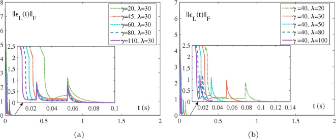
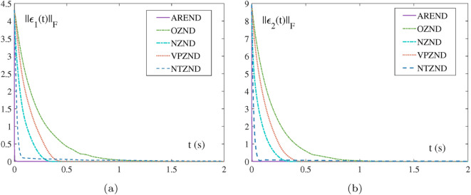
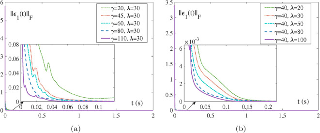
The theoretical analysis in the previous section proves the convergence and robustness of the AREND. In this section, numerical experiments from low-dimensional to high-dimensional matrices are designed to further demonstrate the performance of the proposed model, as well as model validation in the application of the AoA localization. The parameters $\gamma =60$, $\lambda =30$, $\xi =5$, $\alpha =1.5$, $\beta =4$, $\zeta =0.4$, and hyperparameters $\sigma =2$ $\nu =\mu =5$ are utilized throughout the experiments, except where noted specifically. But the tuning of these hyperparameters can only be deployed empirically. Only when addressing the QR factorization, $\nu$ and $\mu$ are adjusted to be 12. In these experiments, the phase in which ZND adjusts the guidance volumes is depicted by the AREND through residual error curve fluctuations, as Figs. 1 and 5a,b shown.

Fig. 1.

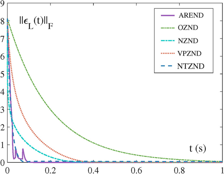
The comparisons of the residual error $\Vert {ϵ}_L{(t)\Vert }_{\text{F}}$ by models solving LR factorization.

Fig. 5.

The comparisons of the residual error $\Vert {ϵ}_L{(t)\Vert }_{\text{F}}$ by AREND-LR (19) solving high dimensional matrix with different values of the two parameters. (a) $\gamma$. (b) $\lambda$.

Instances for evaluation

LR factorization

In order to verify the convergence of the AREND-LR, a following dynamic matrix $M_L(t)\in {\mathbb{R}}^{3\times 3}$ is designed as

$$\begin{array}{c}\hfill \left[\begin{array}{ccc}\text{sin}(t)+3& \text{sin}(2t)& \text{sin}(t)\\ \text{sin}(t)& \text{cos}(t)+5& \text{cos}(2t)\\ \text{sin}(t)-1& \text{cos}(2t+2)& \text{cos}(t)+3\end{array}\right].\end{array}$$

Figure 1 is a comparison of the AREND, OZND, NZND, VPZND, NTZND for the LR factorization in the absence of noise. The OZND converges the latest. The NZND and VPZND converge at around 0.3 s and 0.4 s, respectively. The NTZND cannot adaptively adjust the two guiding volumes and its convergence is incomplete. However, the AREND converges to zero quickly at 0.1 s. The adaptive activation functions of the AREND adjust the level of the two guiding volumes in a very short time. It is demonstrated that the AREND has the excellent performance addressing LR factorization this kind of single-error function problem.

QR factorization

To verify the convergence of the AREND-QR and the effectiveness of the SIC, a dynamic matrix $M_Q(t)\in {\mathbb{R}}^{3\times 3}$ is designed as

$$\begin{array}{c}\hfill \left[\begin{array}{ccc}\text{sin}(3t)& \text{sin}(2t)-2& \text{sin}(t)+1\\ \text{sin}(2t)& \text{cos}(t)& 2\text{cos}(t)\\ -\text{sin}(t)& \text{cos}(2t)& \text{cos}(t)-3\end{array}\right].\end{array}$$

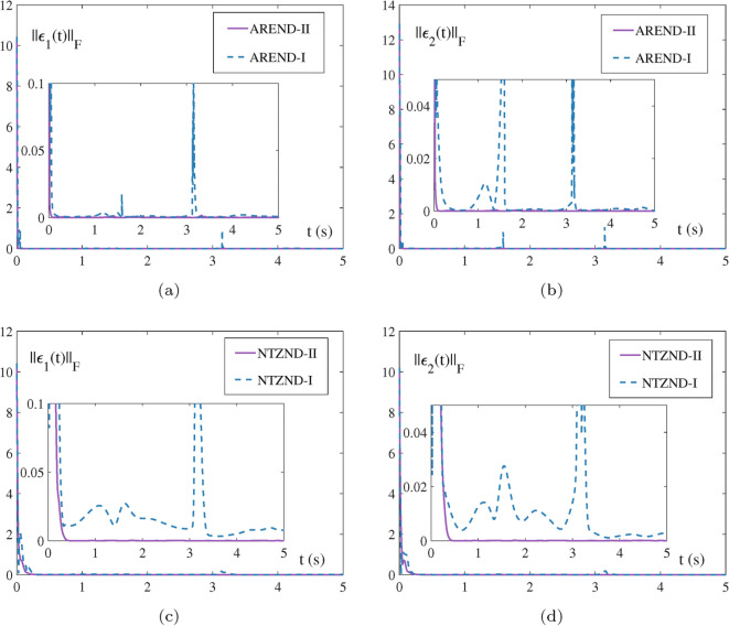
1. Integration-coupling VS. single-integration: In terms of Fig. 2, two ZNDs of IET, the AREND and NTZND, compare the employment of the SIC and single integration. From the surface, the single-integration strategy to solve the problem has precarious convergence. There are a number of up and down oscillations, pointing out that the IET of ZNDs guiding by the single-integration fail to solve the QR factorization this kind of multiple error function problem. On the contrary, the IET of ZNDs all develops stability and convergence capability with the help of the SIC. NTZND-I, the original model, focuses only on the integration feedback from one of the error functions and cannot eliminate the internal errors of the system. NTZND-II, with the help of SIC, enables all the error functions to play a comparable role in solving the system, coupled in the form of cumulative and integral terms, which eliminate the multinomial errors from each other. Furthermore, the adaptive functions activated AREND is more capable of controlling the residual error drop, indicating the superiority of the AREND. Note that the ZNDs of IET are all utilizing the SIC in the following experiments.

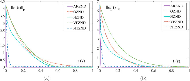
2. Convergence under noise-free case: Refer to Fig. 3, for $\Vert {ϵ}_1{(t)\Vert }_{\text{F}}$ and $\Vert {ϵ}_2{(t)\Vert }_{\text{F}}$, the convergence time of the OZND, NZND, VPZND are around 1s, 0.4s, 0.5s, whereas the NTZND obviously only converges to a small value. Within 0.1s, the two residual errors solved by the AREND converge to zero. The real-time adaptive tuning of the activation functions is justified playing a crucial role in ensuring strong competitiveness of the AREND-QR.

Fig. 2.

The comparisons of residual errors by integration-coupling and single-integration models for solving QR factorization, where II and I represents integration-coupling and single-integration models, respectively. (a) and (c) $\Vert {ϵ}_1{(t)\Vert }_{\text{F}}$. (b) and (d) $\Vert {ϵ}_2{(t)\Vert }_{\text{F}}$.

Fig. 3.

The comparison of residual errors by different models for solving QR factorization. (a) $\Vert {ϵ}_1{(t)\Vert }_{\text{F}}$. (b) $\Vert {ϵ}_2{(t)\Vert }_{\text{F}}$.

High-dimensional situations

LR factorization

To investigate the performance of high dimensional matrix LR factorization in terms of model convergence and robustness in noisy environments, a dynamic matrix $M_L(t)\in {\mathbb{R}}^{4\times 4}$ is designed as

$$\begin{array}{c}\hfill \left[\begin{array}{cccc}\text{sin}(t)+3& \text{sin}(2t)& \text{sin}(t)& -\text{cos}(t)\\ \text{cos}(t)& \text{cos}(t)+5& \text{cos}(2t)& \text{sin}(t)\\ \text{sin}(t)-1& \text{cos}(2t+2)& \text{cos}(t)+3& \text{cos}(2t)\\ \text{cos}(t)& \text{sin}(t+3)& \text{sin}(t-5)& 2-\text{cos}(t)\end{array}\right].\end{array}$$

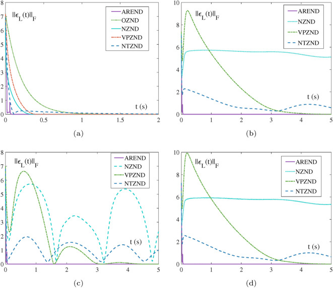
1. Convergence and robustness discussion: Fig. 4 is a comparison of multiple models solving the high dimensional LR factorization. Figure 4a points out that the NZND and VPZND converge in 0.4 s, the AREND has the best convergence performance, converging in 0.1 s. Figure 4b,d indicate that results by all models with the constant noise ${\rho }_c(t)={[10]}^{4\times 4}$ and random noise ${\rho }_r(t)\in {[8,12]}^{4\times 4}$ are generally consistent, Fig. 4c shows under the period noise ${\rho }_p(t)={[10]}^{4\times 4}\times \text{sin}(2t)$, the compared ZNDs fluctuate more. It can be seen that the VPZND is resistant to noise but converges slowly. Only the AREND is the fastest to converge under the three types of noise, and still converges in 0.1s. The activation-coupling contributes to it perfect access to integration information. It turns out the convergence of the AREND-LR is almost unaffected by the noises.

2. Different values of model parameters: Fig. 5 are the comparison of the different values of the two AREND parameters. In Fig. 5a, when $\lambda$ is a fixed value, the larger $\gamma$ is, the faster the adjustment control of the residual error is, and the shorter the time of convergence is. In Fig. 5b, when $\gamma$ is a certain value, the larger the value of $\lambda$, the more rapid the adjustment control of the two guidance volumes becomes, and the more brief the time of convergence is. In summary, the two variables are kept in a certain proportion to increase, the speed of adjustment of the two guiding volumes increases, and the convergence is faster.

Fig. 4.

Multi-model comparisons of the residual error $\Vert {ϵ}_L{(t)\Vert }_{\text{F}}$ for solving high-dimensional matrix LR factorization with different noises. (a) With noiseless. (b) With constant noise ${\rho }_c(t)={[10]}^{4\times 4}$. (c) With period noise ${\rho }_p(t)={[10]}^{4\times 4}\times \text{sin}(2t)$. (d) With random noise ${\rho }_r(t)\in {[8,12]}^{4\times 4}$.

QR factorization

Aiming to explore more performance of the AREND-QR for high-dimensional matrix, a dynamic matrix $M_Q(t)\in {\mathbb{R}}^{5\times 5}$ is designed as

$$\begin{array}{c}\hfill \left[\begin{array}{ccccc}\text{sin}(t)& \text{cos}(t)& \text{sin}(2t)& \text{cos}(2t)& \text{sin}(3t)\\ \text{cos}(3t)& \text{sin}(4t)& \text{cos}(4t)& \text{sin}(5t)& \text{cos}(5t)\\ \text{sin}(6t)& \text{cos}(6t)& \text{sin}(7t)& \text{cos}(7t)& \text{sin}(8t)\\ \text{cos}(8t)& \text{sin}(9t)& \text{cos}(9t)& \text{sin}(10t)& \text{cos}(10t)\\ \text{sin}(11t)& \text{cos}(11t)& \text{sin}(12t)& \text{cos}(12t)& \text{sin}(13t)\\ \end{array}\right].\end{array}$$

1. Under no noise: Fig. 6 is a comparison of the two residual errors of models solving high-dimensional matrix QR factorization. The residual errors by the AREND almost all converge in about 0.01 s. In addition to the role of hyperparameters, the double-coupling of the AREND ensures that the residual error of the solver system decreases rapidly by integrating multiple pieces of information, making the AREND suitable for even high-dimensional matrix.

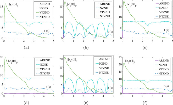
2. Under different noises: Fig. 7 shows a comparison of the two residual error of models under noises. It reveals that the AREND, NTZND, and VPZND are resistant to all three types of noise. However, notices that the VPZND has the disadvantage of being slower to converge, requiring longer time work and more computational cost. The NTZND with integration term undoubtedly gives it some immunity to noise, yet the performance is not satisfactory. But the AREND converges in a very short time about 0.1 s. It is firmly proven that the AREND has an superiority in dealing with QR factorization in noisy environments.

3. Different values of the parameter: Fig. 8 shows the comparison of different values of the control parameters of the AREND. The same as the LR factorization Fig. 5 is that the speed of convergence of the AREND is positively correlated with the values of $\gamma$, $\lambda$. And the difference from the LR factorization is the SIC makes the control adjustment speed of the parameters $\gamma$, $\lambda$ better, and improves the model accuracy.

Fig. 6.

The comparison results by multiple models for solving high-dimensional matrix QR factorization. (a) $\Vert {ϵ}_1{(t)\Vert }_{\text{F}}$. (b) $\Vert {ϵ}_2{(t)\Vert }_{\text{F}}$.

Fig. 7.

The comparisons of residual errors by multiple models for solving high-dimensional matrix QR factorization with multiple large noises. (a) and (d) With constant noise ${\rho }_c(t)={[10]}^{5\times 5}$. (b) and (d) With period noise ${\rho }_p(t)={[10]}^{5\times 5}\times \text{sin}(3t)$. (c) and (f) With random bounded noise ${\rho }_r(t)\in {[8,12]}^{5\times 5}$.

Fig. 8.

The residual error results $\Vert {ϵ}_1{(t)\Vert }_{\text{F}}$ by AREND-QR (22) solving the high dimensional matrix with different values of two parameters. (a) $\gamma$. (b) $\lambda$.

Quantitative analysis

The quantitative experiment results are shown from Tables 1, 2, 3 and 4, which detailedly records the Average Steady-State Residual Error (ASSRE) and Maximal Steady-State Residual Error (MSSRE) when different models solve the high-dimensional LR and QR factorization. The mathematical description of MSSRE is defined as ${lim}_{t\to \infty }sup{\Vert ϵ(t)\Vert }_{\text{F}},t_m\in [t_s,t_{max}]$, and ASSRE is defined as ${\int }_{t_s}^{max}{\Vert ϵ(\delta )\Vert }_{\text{F}}\text{d}\delta /(t_{max}-t_s)$, where t(s) represents the length of time in seconds. In these tables all point out the ZNDs of DCT, such as DPZND⁴¹, DVPEZND⁵², are mostly not suitable for solving LR and QR factorization.

Table 1.

Compare the ASSREs of different models when solving the LR problem.

Model	ASSRE with NF	ASSRE with CN	ASSRE with PN	ASSRE with RN
OZND	$1.60\times {10}^{-3}$	$1.17\times {10}^2$	$1.97\times {10}^1$	$1.33\times {10}^2$
NZND	$5.61\times {10}^{-5}$	$5.17\times {10}^0$	$1.58\times {10}^0$	$5.34\times {10}^0$
VPZND	$5.96\times {10}^{-5}$	$6.40\times {10}^{-3}$	$6.00\times {10}^{-3}$	$8.70\times {10}^{-3}$
NTZND	$2.73\times {10}^{-2}$	$7.29\times {10}^{-1}$	$1.26\times {10}^0$	$7.97\times {10}^{-1}$
DPZND	Divergent	Divergent	Divergent	Divergent
DVPEZND	Divergent	Divergent	Divergent	Divergent
AREND	$\mathbf{2.24}\times {\mathbf{10}}^{-\mathbf{7}}$	$\mathbf{5.41}\times {\mathbf{10}}^{-\mathbf{4}}$	$\mathbf{1.10}\times {\mathbf{10}}^{-\mathbf{3}}$	$\mathbf{1.30}\times {\mathbf{10}}^{-\mathbf{3}}$

NF, CN, PN, and RN signify the noises free, constant noises, period noises, and random noises, respectively. The bold font denotes the best result in the corresponding item

Table 2.

Compare the MSSREs of different models when solving the LR problem.

Model	MSSRE with NF	MSSRE with CN	MSSRE with PN	MSSRE with RN
OZND	$3.60\times {10}^{-3}$	$1.08\times {10}^2$	$5.11\times {10}^1$	$1.35\times {10}^2$
NZND	$7.54\times {10}^{-4}$	$5.15\times {10}^0$	$3.49\times {10}^0$	$5.37\times {10}^0$
VPZND	$7.52\times {10}^{-4}$	$1.66\times {10}^{-2}$	$1.05\times {10}^{-2}$	$2.10\times {10}^{-2}$
NTZND	$2.93\times {10}^{-2}$	$8.50\times {10}^{-1}$	$1.42\times {10}^0$	$9.51\times {10}^{-1}$
DPZND	Divergent	Divergent	Divergent	Divergent
DVPEZND	Divergent	Divergent	Divergent	Divergent
AREND	$\mathbf{4.89}\times {\mathbf{10}}^{-\mathbf{7}}$	$\mathbf{6.60}\times {\mathbf{10}}^{-\mathbf{4}}$	$\mathbf{2.20}\times {\mathbf{10}}^{-\mathbf{3}}$	$\mathbf{6.30}\times {\mathbf{10}}^{-\mathbf{3}}$

NF, CN, PN, and RN signify the noises free, constant noises, period noises, and random noises, respectively. The bold font denotes the best result in the corresponding item

Table 3.

Compare the ASSREs of different models when solving the QR problem.

$ϵ(t)$	Model	ASSRE with NF	ASSRE with CN	ASSRE with PN	ASSRE with RN
${ϵ}_1(t)$	OZND	$9.46\times {10}^{-4}$	$2.66\times {10}^2$	$6.4\times {10}^1$	$3.20\times {10}^2$
	NZND	$8.24\times {10}^{-6}$	$7.09\times {10}^0$	$6.47\times {10}^0$	$7.19\times {10}^0$
	VPZND	$2.75\times {10}^{-6}$	$7.81\times {10}^{-2}$	$5.07\times {10}^{-2}$	$5.07\times {10}^{-2}$
	NTZND	$2.73\times {10}^{-2}$	$7.29\times {10}^{-1}$	$1.26\times {10}^0$	$7.97\times {10}^{-1}$
	DPZND	Divergent	Divergent	Divergent	Divergent
	DVPEZND	Divergent	Divergent	Divergent	Divergent
	AREND	$\mathbf{2.62}\times {\mathbf{10}}^{-\mathbf{6}}$	$\mathbf{4.29}\times {\mathbf{10}}^{-\mathbf{2}}$	$\mathbf{4.01}\times {\mathbf{10}}^{-\mathbf{2}}$	$\mathbf{4.01}\times {\mathbf{10}}^{-\mathbf{2}}$
${ϵ}_2(t)$	OZND	$6.43\times {10}^{-4}$	$3.99\times {10}^2$	$9.13\times {10}^1$	$4.83\times {10}^2$
	NZND	$1.43\times {10}^{-5}$	$8.26\times {10}^0$	$7.97\times {10}^0$	$8.55\times {10}^0$
	VPZND	$2.25\times {10}^{-6}$	$6.59\times {10}^{-2}$	$7.39\times {10}^{-2}$	$7.40\times {10}^{-2}$
	NTZND	$1.33\times {10}^{-2}$	$1.75\times {10}^0$	$1.92\times {10}^0$	$2.17\times {10}^0$
	DPZND	Divergent	Divergent	Divergent	Divergent
	DVPEZND	Divergent	Divergent	Divergent	Divergent
	AREND	$\mathbf{2.22}\times {\mathbf{10}}^{-\mathbf{6}}$	$\mathbf{3.30}\times {\mathbf{10}}^{-\mathbf{2}}$	$\mathbf{1.67}\times {\mathbf{10}}^{-\mathbf{2}}$	$\mathbf{1.67}\times {\mathbf{10}}^{-\mathbf{2}}$

NF, CN, PN, and RN signify the noises free, constant noises, period noises, and random noises, respectively. The bold font denotes the best result in the corresponding item

Table 4.

Compare the MSSREs of different models when solving the QR problem.

$ϵ(t)$	Model	MSSRE with NF	MSSRE with CN	MSSRE with PN	MSSRE with RN
${ϵ}_1(t)$	OZND	$3.90\times {10}^{-3}$	$2.64\times {10}^2$	$9.72\times {10}^1$	$3.20\times {10}^2$
	NZND	$1.65\times {10}^{-4}$	$7.65\times {10}^0$	$7.18\times {10}^0$	$7.82\times {10}^0$
	VPZND	$7.62\times {10}^{-4}$	$1.44\times {10}^{-1}$	$6.05\times {10}^{-2}$	$6.06\times {10}^{-2}$
	NTZND	$1.67\times {10}^{-2}$	$8.50\times {10}^{-1}$	$1.42\times {10}^0$	$9.51\times {10}^{-1}$
	DPZND	Divergent	Divergent	Divergent	Divergent
	DVPEZND	Divergent	Divergent	Divergent	Divergent
	AREND	$\mathbf{5.35}\times {\mathbf{10}}^{-\mathbf{6}}$	$\mathbf{5.16}\times {\mathbf{10}}^{-\mathbf{2}}$	$\mathbf{5.32}\times {\mathbf{10}}^{-\mathbf{2}}$	$\mathbf{5.32}\times {\mathbf{10}}^{-\mathbf{2}}$
${ϵ}_2(t)$	OZND	$2.2\times {10}^{-3}$	$4.00\times {10}^2$	$1.38\times {10}^2$	$4.86\times {10}^2$
	NZND	$1.36\times {10}^{-4}$	$8.56\times {10}^0$	$8.44\times {10}^0$	$8.79\times {10}^0$
	VPZND	$8.03\times {10}^{-5}$	$1.23\times {10}^{-1}$	$1.19\times {10}^{-1}$	$1.19\times {10}^{-1}$
	NTZND	$1.98\times {10}^{-2}$	$2.47\times {10}^0$	$2.54\times {10}^0$	$3.35\times {10}^0$
	DPZND	Divergent	Divergent	Divergent	Divergent
	DVPEZND	Divergent	Divergent	Divergent	Divergent
	AREND	$\mathbf{3.71}\times {\mathbf{10}}^{-\mathbf{6}}$	$\mathbf{4.96}\times {\mathbf{10}}^{-\mathbf{2}}$	$\mathbf{2.32}\times {\mathbf{10}}^{-\mathbf{2}}$	$\mathbf{2.32}\times {\mathbf{10}}^{-\mathbf{2}}$

NF, CN, PN, and RN signify the noises free, constant noises, period noises, and random noises, respectively. The bold font denotes the best result in the corresponding item

1. Performance under noise-free conditions: The AREND performs well under noisy conditions, both on the LR and QR problems. Table 1 shows that AREND has an ASSRE of $2.24\times {10}^{-7}$ for the LR problem, which is much lower than other models such as $1.60\times {10}^{-3}$ for OZND and $2.73\times {10}^{-2}$ for NTZND. The QR problem in Table 3 yields similar results, with AREND’s ASSRE of $2.62\times {10}^{-6}$ and $2.22\times {10}^{-6}$, respectively, which are significantly better than the other models. The results of MSSRE further support this conclusion. In Tables 2 and 4, the MSSRE of the AREND is $4.89\times {10}^{-7}$ for the LR problem, and $5.35\times {10}^{-6}$ and $3.71\times {10}^{-6}$ for the QR problem, which are much smaller than the other comparative models, and show an extremely high accuracy.

2. Performance under constant noise conditions: In the constant noise condition, AREND still performs the best, although the errors of most models have increased. The LR problem in Table 1 shows that AREND has an ASSRE of $5.41\times {10}^{-4}$, which is significantly better than NZND’s $5.17\times {10}^0$ and VPZND’s $6.40\times {10}^{-3}$ For the QR problem (see Table 3), AREND’s ASSRE of $4.29\times {10}^{-2}$ and $3.30\times {10}^{-2}$ is much smaller than OZND’s $2.66\times {10}^2$ and $3.99\times {10}^2$. From the MSSRE point of view, AREND has a MSSRE of $6.60\times {10}^{-4}$ in the LR problem (Table 2), compared to $5.16\times {10}^{-2}$ and $4.96\times {10}^{-2}$ in the QR problem (Table 4). Compared with other models, AREND is less affected by constant noise and shows good robustness.

3. Performance under period noise conditions: Period noise has a large impact on most models, but AREND is still able to maintain a good performance. In Table 1, AREND’s ASSRE for the LR problem is $1.10\times {10}^{-3}$, while the errors for OZND and NTZND are as high as $1.97\times {10}^1$ and $1.26\times {10}^0$, respectively. The ASSRE for the QR problem in Table 3 show a similar trend, with AREND having errors of $4.01\times {10}^{-2}$ and $1.67\times {10}^{-2}$, significantly better than the other models. From the MSSRE point of view, the MSSRE of AREND is $2.20\times {10}^{-3}$ for the LR problem (Table 2) and $5.32\times {10}^{-2}$ and $2.32\times {10}^{-2}$ for the QR problem (Table 4), which compared with the other models, are results prove the periodical robustness under noisy conditions again.

4. Performance under random noise conditions: Random noise is usually the most challenging type of noise, and many models perform poorly or even diverge under this condition. For example, DPZND and DVPEZND diverge under noisy conditions (Tables 1 and 3). However, AREND still maintains a low error. In the LR problem in Table 1, AREND has an ASSRE of $1.30\times {10}^{-3}$, compared to $1.33\times {10}^2$ for OZND and $5.34\times {10}^0$ for NZND. In the QR problem in Table 3, AREND’s ASSRE of $4.01\times {10}^{-2}$ and $1.67\times {10}^{-2}$ again outperforms the other models. The MSSRE results also support this observation, with AREND having an MSSRE of $6.30\times {10}^{-3}$ in the LR problem (Table 2) and values of $5.32\times {10}^{-2}$ and $2.32\times {10}^{-2}$ in the QR problem (Table 4). These results show that the performance of the AREND remains stable under random noise, demonstrating excellent noise immunity.

5. Summary: From the quantitative results, it can be more scientifically seen that the AREND significantly outperforms other models under all noise conditions, whether solving the LR problem or the QR problem. In particular, the AREND demonstrates excellent robustness under complex random and period noise, while other models, such as DPZND and DVPEZND, tend to diverge under noisy conditions. This demonstrates that AREND is one of the most reliable models for dealing with real noise environments and has a wide range of potential applications.

Application in AoA

In this subsection, we design 3-D AoA algorithm localization to validate the AREND. This localization method relies on the base station’s azimuth ${\theta }_i(t)$, elevation ${\tau }_i(t)$ of the base stations to locate mobile target.

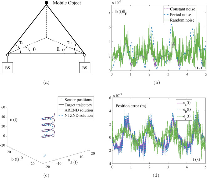
The principle of AoA algorithm localization is illustrated in Fig. 9a. The position of the base station is defined as ${(a_i,b_i,c_i)}^{\text{T}}$, $i=1,2,\cdots ,N$, N depends on the number of base stations. And the position of the target object is given as $(a(t),b(t),c(t){)}^{\text{T}}$. After geometric derivation, the following equation is derived as

$$\begin{array}{c}\hfill \left[\begin{array}{ccc}-\text{tan}{\theta }_1(t)& 1& 0\\ ⋮& ⋮& ⋮\\ -\text{tan}{\theta }_N(t)& 1& 0\\ 0& L_1(t)& -1\\ ⋮& ⋮& ⋮\\ 0& L_N(t)& -1\\ \end{array}\right]\left[\begin{array}{c}a(t)\\ b(t)\\ c(t)\\ \end{array}\right]=\left[\begin{array}{c}{b}_1-a_1\text{tan}{\theta }_1(t)\\ ⋮\\ b_N-a_N\text{tan}{\theta }_N(t)\\ b_1{L}_1(t)-c_1\\ ⋮\\ b_N{L}_N(t)-c_N\\ \end{array}\right],\end{array}$$

where $L_N(t)$ denotes $\text{tan}{\tau }_N(t)\oslash \text{sin}{\theta }_N(t)$, and $\oslash$ stands for element-by-element division. The equation is reduced to $R(t)P(t)=U(t)$. Then the error function is defined as $ϵ(t)=R(t)P(t)-U(t)$, and using the evolution formula (9) and injecting the vector-type noise $\overrightarrow{\rho }(t)$, the NTZND for the 3-dimensional AoA localization is obtained as

$$\begin{array}{c}\hfill \begin{array}{c}\hfill R(t)\dot{P}(t)=-\lambda {\int }_0^t(R(\delta )P(\delta )-U(\delta ))\text{d}\delta -\gamma (R(t)P(t)-U(t))+\overrightarrow{\rho }(t).\end{array}\end{array}$$ 27

Fig. 9.

Validation results of the NTZND (27) and AREND (28) applied in AoA positioning, where the parameters are set to $\gamma =90$, $\lambda =60$. (a) The schematic diagram of the 3-D AOA localization algorithm. (b) The comparison of the residual error by the AREND solving AoA localization with multiple noises, where the constant noise is ${[100]}^{3\times 1}$, the period noise is ${[100]}^{3\times 1}\times \text{sin}(3t)$, the random bounded noise is ${[98,102]}^{3\times 1}$ (c) The comparison of simulated positional solving and target trajectory by the AREND and NTZND under the random noise. (d) The real-time position errors in 3 directions by the AREND solving under the random noise.

Likewise, the AREND for the 3-dimensional AoA localization by the evolution formula (11) is designed as

$$\begin{array}{c}\hfill \begin{array}{cc}\hfill R(t)\dot{P}(t)=& -\lambda \mathrm{\Phi }\left(R,(t),P,(t),-,U,(t),+,\gamma ,{\int }_0^t,\mathrm{\Theta },(,R,(\delta ),P,(\delta ),-,U,(\delta ),),,\text{d},\delta \right)\hfill \\ \hfill & -\gamma \mathrm{\Theta }(R(t)P(t)-U(t))+\overrightarrow{\rho }(t).\hfill \end{array}\end{array}$$ 28

There are 2 base stations set up to simulate the localization process at the following locations: ${[-11,-15,-20]}^{\text{T}}$, ${[-10,-15,-18]}^{\text{T}}$, and the true trajectory of the target object is set: ${[5\text{cos}(5t),5\text{sin}(5t),10t]}^{\text{T}}$. The initial position of the target is assumed as ${[5,0,0]}^{\text{T}}$. As shown in Fig. 9b, under three larger noises, the accuracy of the AREND is in the order of ${10}^{-3}$. In practical localization, random noise is more to be accounted for, and the target trajectory localization solved by the models under the random noise is shown in Fig. 9c. The deviation of the NTZND localization is too heavy, while the solution trajectory of the AREND almost overlaps with the target trajectory. Meanwhile, the position errors of the three directions are shown in Fig. 9d. Previously presented evidence supports the effectiveness and accuracy of the AREND in target localization.

Conclusions

In this paper, an Adaptive and Robust-Enhance Neural Dynamic (AREND), based on the framework of two types of Zeroing Neural Dynamic (ZND), is proposed to improve the performance of solving dynamic matrix LR and QR factorization. And a Strategy of Integration-Coupling (SIC) is proposed for solving multiple error function problems. The simulation experiments firstly demonstrate that the SIC moderates the instability of the Integration-Enhance Type of ZNDs. According to the comparisons, the AREND equipped with the SIC significantly enhances the performance with various environmental disturbances. This means utilizing the proposed model is a more desirable alternative. Revisiting the two types of ZNDs, the AREND has more model superiority undoubtedly, providing valuable tools for solving dynamic problems. Since then, we believe the AREND and SIC can be extended to solve more complex dynamic problems in our future work.

Author contributions

F.H. Zhuang, H.T. He and A.P. Ye were responsible for experimentation and writing of the manuscript, while L.L. Zou was responsible for methodological guidance, financial support, and manuscript revisions.

Funding

This work is supported by National Natural Science Foundation of China under Grant 62272109 and Undergraduate Innovation Team Project of Guangdong Ocean University under Grant CXTD2024011.

Data availability

Code related to this article can be found at https://github.com/Alana2a3/AREND-Code-Implementation, an open-source online code repository hosted at GitHub.

Declarations

Competing interests

The authors declare no competing interests.

Ethical standard

All data used in this paper are publicly available and no consent was required for their use.

References

- 1.Gohberg, I., Kaashoek, M.A. & Spitkovsky, I.M. An overview of matrix factorization theory and operator applications. in (Gohberg, I., Manojlovic, N., dos Santos, A.F., Eds.) Factorization and Integrable Systems. Operator Theory: Advances and Applications, 1–102. (Springer, 2003).
- 2.Srebro, N. (2004). Learning with matrix factorizations
- 3.Koren, Y., Bell, R. & Volinsky, C. Matrix factorization techniques for recommender systems Computer 42(8), 30–37 (2009).
- 4.Xiao, T. & Shen, H. Neural variational matrix factorization for collaborative filtering in recommendation systems. Appl. Intell.49, 3558–3569 (2019). [Google Scholar]
- 5.Al-Harthi, N., Alomairy, R., Akbudak, K., Chen, R., Ltaief, H., Bagci, H. & Keyes, D. (2020). Solving Acoustic Boundary Integral Equations Using High Performance Tile Low-Rank LU Factorization. In: High Performance Computing: 35th International Conference, pp 209-229
- 6.Higham, D. J., Higham, N. J. & Pranesh, S. Random matrices generating large growth in LU factorization with pivoting. SIAM J. Matrix Anal. Appl.42(1), 185–201 (2021). [Google Scholar]
- 7.Lindquist, N., Gates, M., Luszczek, P. & Dongarra, J. (2022). Threshold Pivoting for Dense LU Factorization. in 2022 IEEE/ACM Workshop on Latest Advances in Scalable Algorithms for Large-Scale Heterogeneous Systems. IEEE, pp 34-42
- 8.Zhao, J., Wen, Y., Luo, Y., Jin, Z., Liu, W. & Zhou, Z. (2021). SFLU: Synchronization-Free Sparse LU Factorization for Fast Circuit Simulation on GPUs. in 2021 58th ACM/IEEE Design Automation Conference. IEEE, pp 37-42
- 9.Kwasniewski, G., Ben-Nun, T., Ziogas, AN., Schneider, T., Besta, M. & Hoefler, T. (2021). On the parallel I/O Optimality of Linear Algebra Kernels: Near-Optimal LU Factorization. In Proceedings of the 26th ACM SIGPLAN Symposium on Principles and Practice of Parallel Programming, pp 463-464
- 10.Wang, T., Li, W., Pei, H., Sun, Y., Jin, Z. & Liu, W. (2023). Accelerating Sparse LU Factorization with Density-Aware Adaptive Matrix Multiplication for Circuit Simulation. In 2023 60th ACM/IEEE Design Automation Conference. IEEE, pp 1-6
- 11.Zhang, S., Baharlouei, E. & Wu, P. (2020). High accuracy matrix computations on neural engines: Study of QR factorization. in Proceedings of the 29th International Symposium on High-Performance Parallel and Distributed Computing, pp 17–28
- 12.Shen, Y. & Ypma, T. J. Solving separable nonlinear least squares problems using the QR factorization. J. Comput. Appl. Math.345, 48–58 (2019). [Google Scholar]
- 13.Hebling, G. M., Massignan, J. A., Junior, J.B.-L. & Camillo, M. H. Sparse and numerically stable implementation of a distribution system state estimation based on multifrontal QR factorization. Electr. Power Syst. Res.189, 106734 (2020). [Google Scholar]
- 14.Fukaya, T., Kannan, R., Nakatsukasa, Y., Yamamoto, Y. & Yanagisawa, Y. Shifted Cholesky QR for computing QR factorization of ill-conditioned matrices. SIAM J. Sci. Comput.42(1), A477–A503 (2020). [Google Scholar]
- 15.Faifer, M., Laurano, C., Ottoboni, R. & Toscani, S. Adaptive polynomial harmonic distortion compensation through iteratively updated QR factorization. IEEE Trans. Instrum. Meas.72, 1–10 (2023).37323850 [Google Scholar]
- 16.Danaei, K. et al. 3D inversion of gravity data with unstructured mesh and least-squares QR-factorization (LSQR). J. Appl. Geophys.206, 104781 (2022). [Google Scholar]
- 17.Cao, X., Chen, Y., Zhao, Q., Meng, D., Wang, Y., Wang, D. & Xu, Z. (2015). Low-rank matrix factorization under general mixture noise distributions. in Proceedings of the IEEE International Conference on Computer Vision. IEEE, 1493–1501
- 18.Zhou, N. et al. Robust semi-supervised data representation and imputation by correntropy based constraint nonnegative matrix factorization. Appl. Intell.53(10), 11599–11617 (2023). [Google Scholar]
- 19.Connolly, M. P. & Higham, N. J. Probabilistic Rounding Error Analysis of Householder QR Factorization. SIAM J. Matrix Anal. Appl.44(3), 1146–1163 (2023). [Google Scholar]
- 20.Thomas, E. & Sarin, V. QR decomposition based low rank approximation for Gaussian process regression. Appl. Intell.53(23), 28924–28936 (2023). [Google Scholar]
- 21.Zhang, L., Liu, Z., Pu, J. & Song, B. Adaptive graph regularized nonnegative matrix factorization for data representation. Appl. Intell.50, 438–447 (2020). [Google Scholar]
- 22.Li, T., Zhang, R., Yao, Y., Liu, Y. & Ma, J. (2024). Link prediction using deep autoencoder-like non-negative matrix factorization with L21-norm. Appl. Intell. 1–26.
- 23.Ye, A., Xiao, X., Xiao, H., Jiang, C. & Lin, C. (2024). ACGND: Towards lower complexity and fast solution for dynamic tensor inversion. Complex Intell. Syst. 1–15.
- 24.Tong, K., Jiang, C., Gui, J. & Cao, Y. (2024). Taxonomy driven fast adversarial training. in Proceedings of the AAAI Conference on Artificial Intelligence, 5233–5242.
- 25.He, H., Jiang, C., Xiao, X. & Wang, G. A dynamic matrix equation solution method based on NCBC-ZNN and its application on hyperspectral image multi-target detection. Appl. Intell.53, 22267–22281 (2023). [Google Scholar]
- 26.Jiang, C. & Xiao, X. Norm-based adaptive coefficient znn for solving the time-dependent algebraic riccati equation. IEEE/CAA J. Automatica Sinica10(1), 298–300 (2023). [Google Scholar]
- 27.Lin, C., Mao, X., Qiu, C. & Zou, L. DTCNet: Transformer-CNN distillation for super-resolution of remote sensing image. IEEE J. Sel. Top. Appl. Earth Obs. Remote Sens.10.1109/JSTARS.2024.3409808 (2024). [Google Scholar]
- 28.Gu, X., Chen, X., Yang, M., Du, Y. & Tang, M. Bi-DNE: Bilayer evolutionary pattern preserved embedding for dynamic networks. Complex Intell. Syst.10, 3763–3788 (2024). [Google Scholar]
- 29.Predić, B. et al. Cloud-load forecasting via decomposition-aided attention recurrent neural network tuned by modified particle swarm optimization. Complex Intell. Syst.10, 2249–2269 (2024). [Google Scholar]
- 30.Wang, C., Sun, Y., Ma, X., Chen, Q., Gao, Q & Liu, X. (2024). Multi-agent dynamic formation interception control based on rigid graph. Complex Intell. Syst. 10.1007/s40747-024-01467-3
- 31.Zhang, S., Lu, S., He, Q. & Kong, F. Time-varying singular value decomposition for periodic transient identification in bearing fault diagnosis. J. Sound Vib.379, 213–231 (2016). [Google Scholar]
- 32.Ghaderyan, P., Abbasi, A. & Ebrahimi, A. Time-varying singular value decomposition analysis of electrodermal activity: A novel method of cognitive load estimation. Measurement126, 102–109 (2018). [Google Scholar]
- 33.Uhlig, F. (2022). Adapted AZNN methods for time-varying and static matrix problems. arXiv preprint arXiv:2209.10002
- 34.Uhlig. F. (2024). Zhang neural networks: An introduction to predictive computations for discretized time-varying matrix problems. Numerische Mathematik 1–49.
- 35.Xiao, L., He, Y., Li, Y. & Dai, J. Design and analysis of two nonlinear ZNN models for matrix LR and QR factorization. IEEE Trans. Ind. Inform.19(6), 7424–7434 (2023). [Google Scholar]
- 36.Zhang, Y., Yi, C., Guo, D. & Zheng, J. Comparison on Zhang neural dynamics and gradient-based neural dynamics for online solution of nonlinear time-varying equation. Neural Comput. Appl.20, 1–7 (2011). [Google Scholar]
- 37.Jin, L., Zhang, Y., Li, S. & Zhang, Y. Noise-tolerant ZNN models for solving time-varying zero-finding problems. IEEE Trans. Autom. Control62(2), 992–997 (2016). [Google Scholar]
- 38.Chen, D. & Zhang, Y. Robust zeroing neural-dynamics and its time-varying disturbances suppression model. IEEE Trans. Neural Netw. Learn Syst.29(9), 4385–4397 (2017). [DOI] [PubMed] [Google Scholar]
- 39.Wei, L., Jin, L. & Luo, X. Noise-suppressing neural dynamics for time-dependent constrained nonlinear optimization. IEEE Trans. Syst. Man Cybern. Syst.52(10), 6139–6150 (2022). [Google Scholar]
- 40.Xiao, L. et al. Parameter-changing and complex-valued zeroing neural-network for time-varying complex linear matrix equations. IEEE Trans. Ind. Inform.17(10), 6634–6643 (2021). [Google Scholar]
- 41.Xiao, L., Li, X., Huang, W. & Jia, L. Finite-time solution of time-varying tensor inversion by a novel dynamic-parameter zeroing neural-network. IEEE Trans. Ind. Inform.18(7), 4447–4455 (2021). [Google Scholar]
- 42.Li, Z., Zhang, Y., Ming, L., Guo, J. & Katsikis, V. N. Real-domain QR decomposition models using zeroing neural network for time-varying matrices. Neurocomputing448, 217–227 (2021). [Google Scholar]
- 43.Chen, J. & Zhang, Y. Online singular value decomposition of time-varying matrix via zeroing neural dynamics. Neurocomputing383, 314–323 (2020). [Google Scholar]
- 44.Katsikis, V. N., Mourtas, S. D., Stanimirović, P. S. & Zhang, Y. Solving complex-valued time-varying linear matrix equations via QR decomposition. IEEE Trans. Neural Netw. Learn Syst.33(8), 3415–3424 (2021). [DOI] [PubMed] [Google Scholar]
- 45.Huang, H. et al. Modified Newton integration neural algorithm for dynamic complex-valued matrix pseudoinversion applied to mobile object localization. IEEE Trans. Ind. Inform.17(4), 2432–2442 (2020). [Google Scholar]
- 46.Noroozi, A., Oveis, A. H., Hosseini, S. M. & Sebt, M. A. Improved algebraic solution for source localization from TDOA and FDOA measurements. IEEE Wireless Commun. Lett.7(3), 352–355 (2018). [Google Scholar]
- 47.Dempster, A. G. & Cetin, E. Interference localization for satellite navigation systems. Proc. IEEE104(6), 1318–1326 (2016). [Google Scholar]
- 48.Jiang, C., Wu, C., Xiao, X. & Lin, C. Robust neural dynamics with adaptive coefficient for dynamic matrix square root. Complex Intell. Syst.9(4), 4213–4226 (2023). [Google Scholar]
- 49.Zhang, D., Lee, T. C., Sun, X. M. & Wu, Y. Practical regulation of nonholonomic systems using virtual trajectories and LaSalle invariance principle. IEEE Trans. Syst. Man Cybern. Syst.50(5), 1833–1839 (2018). [Google Scholar]
- 50.Rosenvasser, Y. N., Polyakov, E. Y. & Lampe, B. P. Application of laplace transformation for digital redesign of continuous control systems. IEEE Trans. Autom. Control44(4), 883–886 (1999). [Google Scholar]
- 51.Oppenheim, A.V., Willsky, A.S. & Nawab, S.H. Signals and Systems. (Prentice Hall Inc., 1997).
- 52.Xiao, L., Li, X., Cao, P., He, Y., Tang, W., Li, J. & Wang, Y. (2023). Dynamic-varying parameter enhanced ZNN model for solving time-varying complex-valued tensor inversion for image encryption. IEEE Trans. Neural Netw. Learn Syst. 1–10. [DOI] [PubMed]
Associated Data
This section collects any data citations, data availability statements, or supplementary materials included in this article.
Data Availability Statement