Abstract
Hierarchical structures and heterogeneous materials are found in many natural and engineered systems including additive manufacturing, alternative energy, biology and polymer science. Though the structure–function relationship is important for developing more advanced materials, structural characterization over broad length scales often requires multiple complementary measurements. Neutron far-field interferometry aims to enable multi-scale characterization by combining the best of neutron imaging with small-angle neutron scattering (SANS) via dark-field imaging. The microstructure, nominally from 1 nm to 10 μm, is averaged over each volume element ~(50 μm)3 in the sample, resulting in a ‘tomographic SANS’ measurement. Unlike in small-angle scattering, there are few analytical models to fit dark-field imaging data to extract properties of the microstructure. Fortunately, the dark field and SANS are related through a single Hankel transform. In this work, we discuss the development of a Python-based library, correlogram-tools, that makes use of existing small-angle scattering models and a numerical implementation of the Hankel transform to simulate dark-field interferometry data. We demonstrate how this software can be used to inform researchers of viable sample sets for interferometry experiments, analyze interferometry data, and simulate raw and reconstructed interferometry images for the training of more advanced segmentation models and analysis protocols.
Keywords: neutron dark-field imaging, small-angle neutron scattering, neutron interferometry, simulation software
Graphical Abstract
1. Introduction
Small-angle and ultra-small-angle neutron scattering (SANS and USANS) are used to characterize structure between 1 nm and 10 μm through the measurement of Fourier power spectra or, rather, an inverse-space representation of real-space correlation functions (Jeffries et al., 2021). The spectra are often fitted with empirical or theoretical models to extract quantitative information about the shapes, sizes, self-assembly and interactions of scatterers in the sample and are analyzed with a combination of a priori knowledge of the system and information from complementary characterization measurements. SANS provides a representation of the bulk microstructure ensemble-averaged over the volume of the sample through which the beam passes. This means that it can be difficult to deconvolute complex scattering signals from the study of heterogeneous materials. However, heterogeneity is ubiquitous in real-world materials, from additive manufacturing (Tan et al., 2021; Brooks et al., 2018), alternative energy (Nie et al., 2021), biology (Huang et al., 2019; Weigandt et al., 2009), colloidal science (Han et al., 2022), construction (Allen et al., 2007; Kupwade-Patil et al., 2020), geology (Wang et al., 2013; Bahadur et al., 2014), medicine, polymer science (Xu et al., 2019; White & Calabrese, 2022) and more, thus demanding a new measurement methodology. Neutron imaging, on the other hand, directly probes heterogeneous materials down to ~10 μm to 100 μm but is unable to resolve structural information at the length scales measured with small-angle scattering. Grating-based neutron interferometry (Pfeiffer et al., 2006) offers an advantage in that it captures small-angle scattering information via the dark-field signal (Strobl et al., 2008) with a spatial resolution provided by neutron imaging. Both SANS and dark-field imaging probe the autocorrelation function of the density distribution of a material. SANS measures a Fourier transform of the autocorrelation function while the dark field measures a real-space projection or Abel transform of the autocorrelation function in spherically symmetric systems (Bakker et al., 2020; Andersson et al., 2008; Strobl, 2015).
The dark field is measured by a loss in visibility of the interference pattern, or moiré pattern, at the detector and can be accessed through different beamline geometries. Two primary geometries are far-field (the focus of this work) and Talbot–Lau (Pfeiffer et al., 2006; Kim, Kim et al., 2022) interferometers. We refer the reader to work by Strobl et al. (2017) for a more detailed review of these instruments, which can all benefit from the one-dimensional simulations discussed in this work. Referring to Fig. 1(a), two phase gratings of a far-field interferometer [instrumentation described by Kim et al. (2023)] impart an interference or moiré pattern on the detector that results in a transmission image of the sample convoluted with the sinusoidal moiré pattern. The reduction in visibility of the moiré pattern is due to small-angle scattering. In this configuration, the interferometer is sensitive only to scattering in the direction of modulation of the moiré pattern [x axis in Fig. 1(a)]. Although not currently implemented in the tool that we introduce here, the development of multi-directional gratings and the inclusion of polarization analysis also broaden the sensitivity of the technique to anisotropic structure and magnetic properties of materials (Valsecchi et al., 2020, 2021; Busi et al., 2023). The autocorrelation length ξ, which is the microstructural length scale being probed, depends on the parameters of the interferometer (Strobl, 2015; Wen et al., 2008):
| (1) |
where λ is the source wavelength and PD is the period of the moiré pattern at the detector. The parameter Z is the distance from the sample to the detector. In cases of some Talbot–Lau configurations, the definition of this distance will depend on the configuration of the sample and gratings (Strobl, 2015; Strobl et al., 2017; Yashiro et al., 2010). Different ranges of autocorrelation lengths, i.e. length scales of scattering, can be accessed by varying one or more of these parameters.
Figure 1.
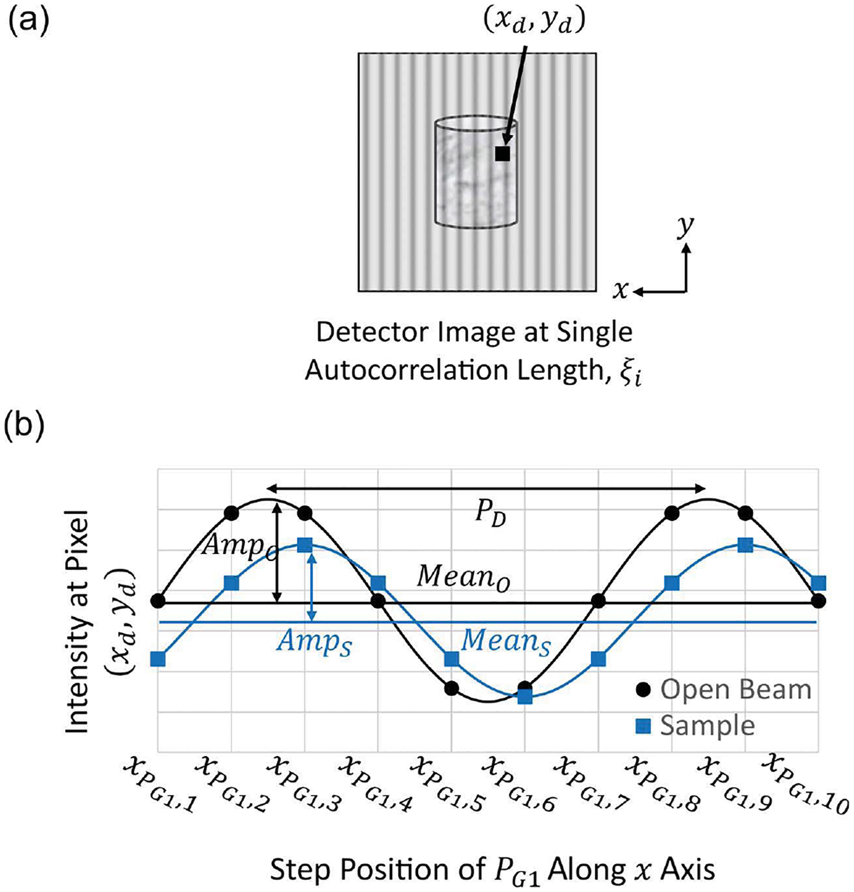
(a) Example of the detector image taken for a sample at a set autocorrelation length which demonstrates the convoluted transmission image of the sample and sinusoidal moiré pattern created by the phase gratings. (b) Neutron intensity at a single pixel location in both sample and open beam images as the first phase grating is translated along the x direction. PG1 refers to the first phase grating in the instrumentation described by Kim et al. (2023).
The moiré pattern can be approximated as a sine curve at each pixel location in the image [e.g. (xd, yd) in Fig. 1] if phase step scanning is performed during the measurement. A phase step scan, which is performed by translating one of the phase gratings through at least one period of the moiré pattern, allows the user to characterize this pattern, as shown in Fig. 1(b), with and without the presence of the sample. Without a phase step scan, a larger area must be used to characterize the pattern, resulting in a loss in spatial resolution. Changes to this sinusoidal pattern of phase shift, mean and visibility are then used to reconstruct three sets of images collected simultaneously by grating-based neutron interferometry: differential phase contrast, attenuation and dark field, respectively (Strobl et al., 2008; Pfeiffer et al., 2006). The visibility, V, of each sine curve is defined as the ratio of the amplitude to the mean:
| (2) |
where i represents either the sample (s) or the open beam (o). Small-angle scattering imparted by the sample at the autocorrelation length of the measurement results in a loss in visibility of this curve, which is quantified in the dark-field intensity by
| (3) |
The dark-field image is measured in real space, but it is a projection of the autocorrelation function, γ(r), of the density distribution. The two-dimensional projection function of the autocorrelation function, G(z), is related to γ(r) through an Abel transform (Andersson et al., 2008). The dark-field signal, DF, from interferometry measurements is related to this projection function through the following equation (Strobl, 2015; Bakker et al., 2020):
| (4) |
where λ is the wavelength of the source, ξ is the autocorrelation length and t is the sample thickness. If the sample is structurally homogeneous along the direction parallel to the beam path, the integral can be simplified with sample thickness t. Finally, we define the relationship between the dark field and small-angle scattering which are related via a single Hankel transform (Bakker et al., 2020; Andersson et al., 2008):
| (5) |
where J0 is the zeroth-order Bessel function of the first kind.
A challenging aspect of modeling dark-field neutron imaging data is the limited number of analytical models, since many of the integrals expressing the projection of the autocorrelation function do not have an analytical form. However, the visibility is analogous to the polarization measured in spin-echo small-angle neutron scattering (SESANS) (Andersson et al., 2008; Strobl, 2015), so the same models developed within the SESANS community can be applied in the dark-field interferometry community and vice versa. Yet, knowledge of the appropriate autocorrelation function and use of the relevant transform to solve for the projection function are required. This is often an arduous task without the aid of mathematical software (Andersson et al., 2008). Therefore, few analytical models exist in either community. Existing analytical models include those for spheres, which have been used to fit the dark-field signal due to porosity in metal additive manufactured materials (Brooks et al., 2018, 2017; Bacak et al., 2020), micellar structures in milks (Kim, Valsecchi et al., 2022) and nanoparticles in solution (Kim et al., 2019; Strobl et al., 2016; Strobl, 2015). Random-two-phase and fractal models have been used to fit the dark-field signal from silica powders (Kim et al., 2019; Harti et al., 2018) and milk gels (Kim, Valsecchi et al., 2022), and an oriented period bar model was used to describe the dark-field signal from a silicon comb or Ronchi grating (Kim, Kim et al., 2022). For a more thorough derivation of these and other available analytical models, we refer the reader to the work of Andersson et al. (2008). Yet, there still does not exist a library of models in the dark-field community as large as that for small-angle scattering.
Neutron dark-field imaging enables the collection of microstructural information captured by small-angle scattering at each pixel location by extraction of the dark-field curves through a stack of images acquired at multiple autocorrelation lengths. This effectively provides spatially resolved SANS-like data (Bacak et al., 2020), making dark-field imaging useful for characterization of complex and real-world materials. Three-dimensional reconstructions of materials with a resolution on the order of 50 μm will enable a ‘tomographic SANS’ measurement, but also provides a big-data challenge in the analysis of up to 109 correlograms depending on the sample size within the available field of view. Traditional analysis approaches, especially manual fitting, quickly become infeasible at this scale. Rather, more advanced segmentation or machine-learning models will be critical to ensuring efficient analysis and interpretation of this data stream. Yet the available experimental data are still insufficient for effective training of such models. Moreover, it is impractical to collect the large amounts of data necessary for model training across wide ranges of measurement and sample conditions for each future experiment. In response, we developed correlogram-tools, a Python-based package for the simulation and eventual analysis of dark-field interferometry data. This tool not only enables the generation of large training sets for machine-learning models and advanced segmentation algorithms but also enables us to make use of an existing library of small-angle scattering models of different types of materials and structures to simulate data from both small-angle scattering and dark-field measurements.
2. Methods
The correlogram-tools package builds on existing SESANS tools in SasView (http://www.sasview.org/) but adds interferometry-specific parameters that enable simulation of realistic dark-field spectra and images. As an alternative to solving for analytical models, the SESANS community has implemented a numerical Hankel transform in SasView, detailed and previously validated by Bakker et al. (2020), which enables fitting and analysis of their one-dimensional datasets with the library of over 70 models included in the small-angle scattering software (Bakker et al., 2020; Doucet et al., 2022). The same models and parameters used to fit SANS data are simply transformed to the real space following equation (5) and used to fit the SESANS data. Moreover, these SESANS spectra are normalized by wavelength and sample path length into standardized forms for analysis independent of instrumentation. However, this limits our ability to use these models to further understand the full scope of feasible samples and measurement conditions. The correlogram-tools package adds to the SESANS numerical implementation of the Hankel transform in two ways. First, the program uses wavelength and sample path length to scale the loss in visibility or dark-field spectra as shown in equation (4). The current version of correlogram-tools assumes a single microstructure along the beam path through the material, and so the integral of equation (4) is simplified to a scaling by sample path length t. Similarly to the SESANS tools, dark-field spectra can be simulated with any of the small-angle scattering form factors and structure factors provided in SasView. However, correlogram-tools then makes it possible to simulate a realistic loss in visibility that is indicative of the signal we would observe in neutron dark-field imaging measurements.
The second added functionality is that correlogram-tools transforms these modeled dark-field spectra, along with instrument geometry and measurement conditions specific to grating-based interferometers, to generate simulated raw and reconstructed dark-field and attenuation images from a specific instrument. The program incorporates instrument geometry (e.g. sample-to-detector distance, interferometer length and available grating periods), detector resolution and noise to introduce optical corrections (e.g. magnification and image blur) for generation of realistic and instrument-specific simulated images that inform researchers of the capabilities and limitations of their instrument. Fig. 2 shows a schematic of the full simulation pipeline. For an in-depth description of the required inputs, file formats and other usage instructions, we refer the reader to the correlogram-tools source code and documentation (Wolf et al., 2023). Here we provide a simplified overview of the simulation pipeline that captures the image-generation functionality of the program.
Figure 2.
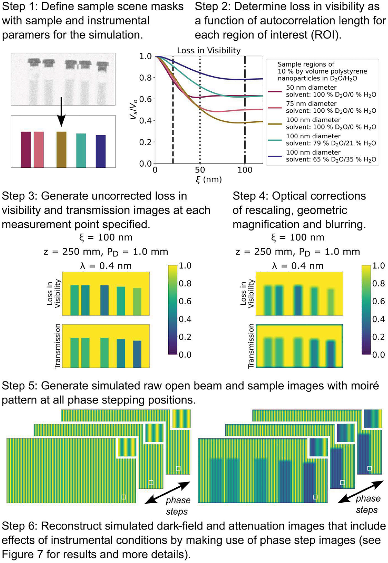
Flow chart of the image-simulation pipeline of correlogram-tools.
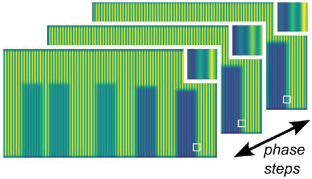
In step 1, the user produces a region of interest (ROI) mask that represents a desired sample scene where each ROI classifies a sample region with a unique microstructure. In this example, five sample vials are simplified to rectangular ROIs with constant path length. Sample vials with a circular rather than rectangular cross-section can be modeled by employing a second mask (not shown) that defines path length variation by pixel. In the following step, correlogram-tools converts the microstructural information, for each ROI, into the one-dimensional loss in visibility spectra. The loss in visibility of step 2 in Fig. 2 shows data for a series of polystyrene nanoparticle dispersions in water. Next, the program determines the measurement conditions of the simulated image acquisitions, including the moiré period, sample position and wavelength, that will achieve the requested autocorrelation lengths as defined in equation (1). These points are denoted by the dashed vertical lines on the loss in visibility plot (three autocorrelation lengths chosen for this example). The available set or range of accepted values for the neutron source wavelength, sample-to-detector distance and moiré period are specified in the instrument configuration. The user may then place additional constraints on the simulation. For example, one could request a simulation that modulates only the sample-to-detector distance to scan the requested autocorrelation lengths. At step 3, the simulated losses in visibility and transmission values for each ROI are converted into the uncorrected images at every autocorrelation length by matching the ROI specified in each pixel to the appropriate intensity from the simulated loss in visibility, and rescaling each image to the appropriate measurement wavelength and each pixel to the appropriate path length. In this example shown in Fig. 2, the loss in visibility and transmission images are shown for a single autocorrelation length, 100 nm. The loss in visibility in each sample ROI can be related to the values shown in the one-dimensional spectra by following the vertical dot–dashed line. The effect of increasing light water in the solvent phase of this example also results in a reduction of transmission from left to right in the samples and is estimated using the periodictable (Kienzle, 2021) Python package.
In the remaining steps of the simulation pipeline, sample and instrumental effects including noise, geometric magnification and geometric blur are added to the uncorrected ground truth images. This allows the generation of simulated images that include many of the features we would see from experimental data. Because the user specifies the relevant instrument details, this tool is applicable to a range of grating interferometer configurations and equipment (e.g. detector resolution). In step 4 of Fig. 2, these optical corrections are most visible in the blurred edges of the sample ROIs. First, the rescaling is considered with the geometric magnification that is given by
| (6) |
where L is the distance from the aperture to the detector and Z is the distance from the sample to the detector. This is important as the apparent size of the sample objects and their blur will increase as the sample is translated away from the detector to measure the dark-field signal at larger autocorrelation lengths. Then, the geometric blurring is implemented by convolution with the geometric blurring kernel B over the geometric magnification. The kernel in this case has a disk shape with a geometric radius given by
| (7) |
where w is the size of aperture, px is the effective pixel size of the image and λg is the blur radius in pixels. Fig. 2 shows these multiple optical corrections in a single step, but Fig. 3 provides a more detailed breakdown of each operation on the images.
Figure 3.
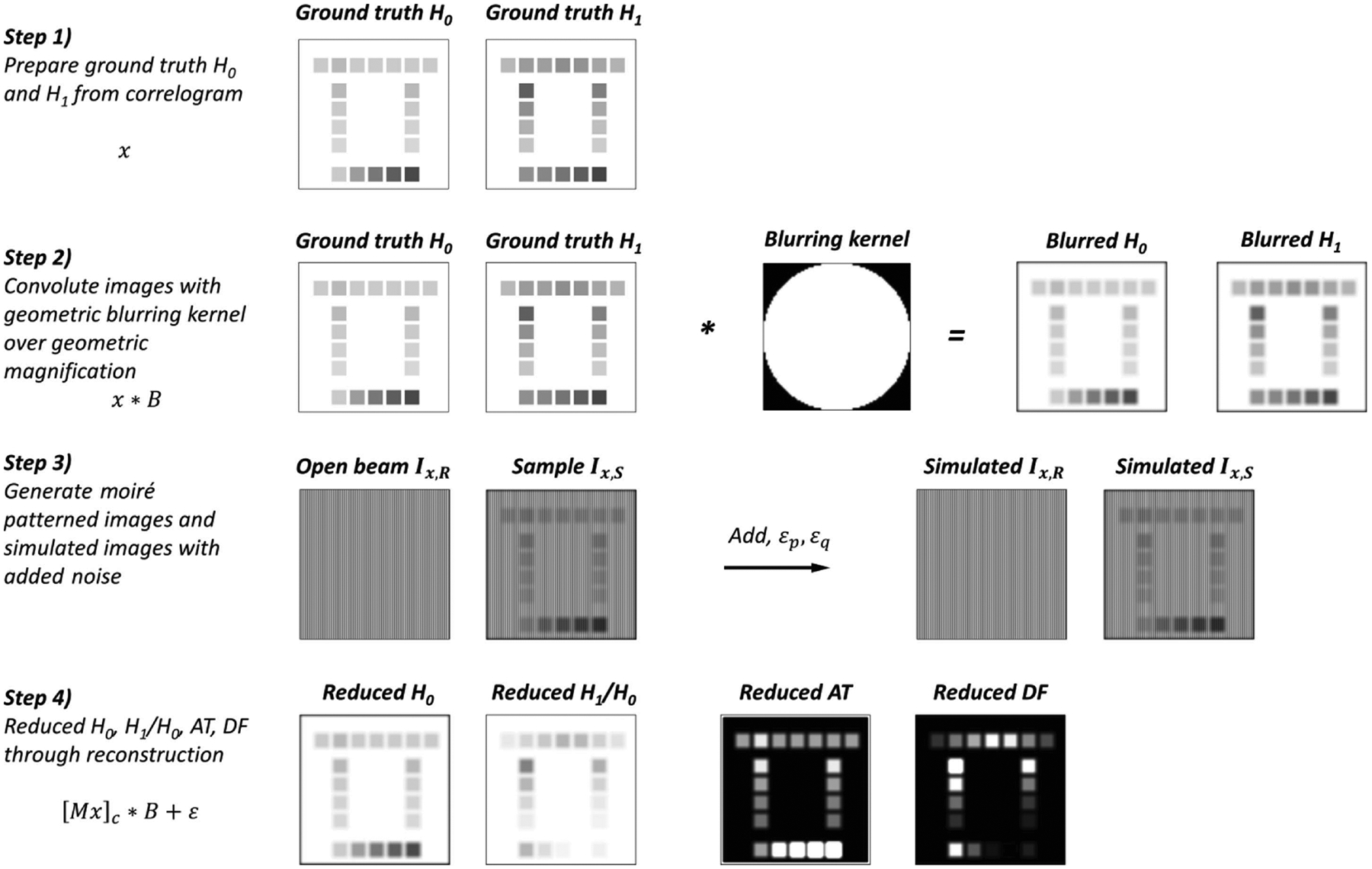
Detailed breakdown of optical corrections during simulations. The result in step 4 is the case of D4 in Fig. S1. H0 represents the transmission (Means/Meano), H1/H0 represents the loss in visibility Vs/Vo, ATrepresents the attenuation [− ln(Means/Meano)], and DF represents the dark-field [− ln(Vs=Vo)] signals and/or images.
The Means and Amps in each ROI of the blurred images x * B are then used to generate the moiré patterned images at the phase step conditions as shown in step 5 of Fig. 2. Applying the optical corrections of geometric magnification prior to the addition of the moiré pattern is important to ensure that the apparent size of the sample objects and the size of the moiré image are correctly proportioned according to the resolution and pixel size of the detector. Both the attenuation and the dark-field images are used to generate the sample image multiplied with the moiré, and then an additional open beam image without the sample objects is generated. Next, the quantized noise εq and the phase step noise εp are added to moiré patterned images and both are assumed to follow the Gaussian distribution
| (8) |
where σ is the standard deviation and μ is the mean. The phase step noise accounts for the variation in the phase step position and non-uniform beam profile in the simulated images. However, the reconstruction step of the code that generates dark-field and transmission images from the simulated raw images does not yet take this into account. Setting μ = 0 assumes that the phase steps can be exactly repeated. These pairs of open beam and sample images represent the raw data that would be collected during a neutron dark-field imaging experiment. An implementation of the reconstruction algorithm described by Marathe et al. (2014) is then used to generate the simulated reconstructed dark-field and attenuation images that now include optical and other instrumental corrections.
3. Results and discussion
In this section, we use correlogram-tools to probe the sample space and explore dark-field neutron imaging feasibility across a wide variety of materials and conditions that can be measured with neutron dark-field imaging. The inclusion of wavelength and sample path length with existing small-angle scattering models enables simulation of realistic one-dimensional dark-field spectra from a specific material to understand the expected signal strength. Figs. 4–6 explore the impact of instrument parameters, sample composition and sample configuration in one-dimensional correlogram space. Though the simulated spectra are important for determining sample viability, they also serve as critical input for the full instrument simulation that considers measurement artifacts induced by instrument configuration and statistical noise. In Fig. 2 of the Methods, we road-mapped the process by which we simulate the instrument raw data based on the one-dimensional inputs, a generated sample mask and the instrument configuration. Fig. 7 takes a closer look at the effects of moiré period and the sample-to-detector distance on the artifacts introduced in both raw and reconstructed attenuation and dark-field images.
Figure 4.
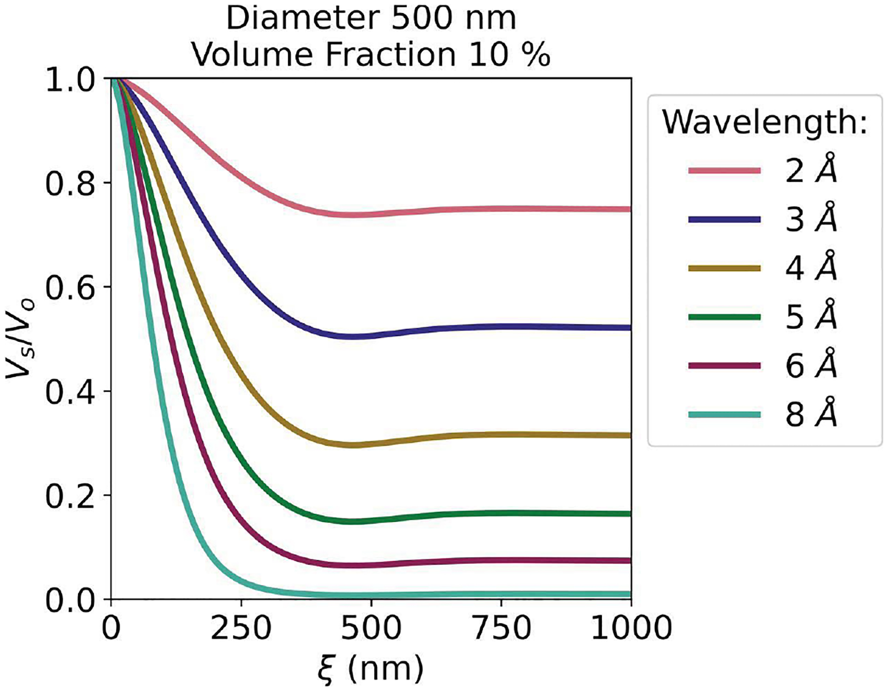
Simulated loss in visibility for polystyrene nanoparticles in heavy water with a path length of 1 mm and varied neutron wavelengths.
Figure 6.
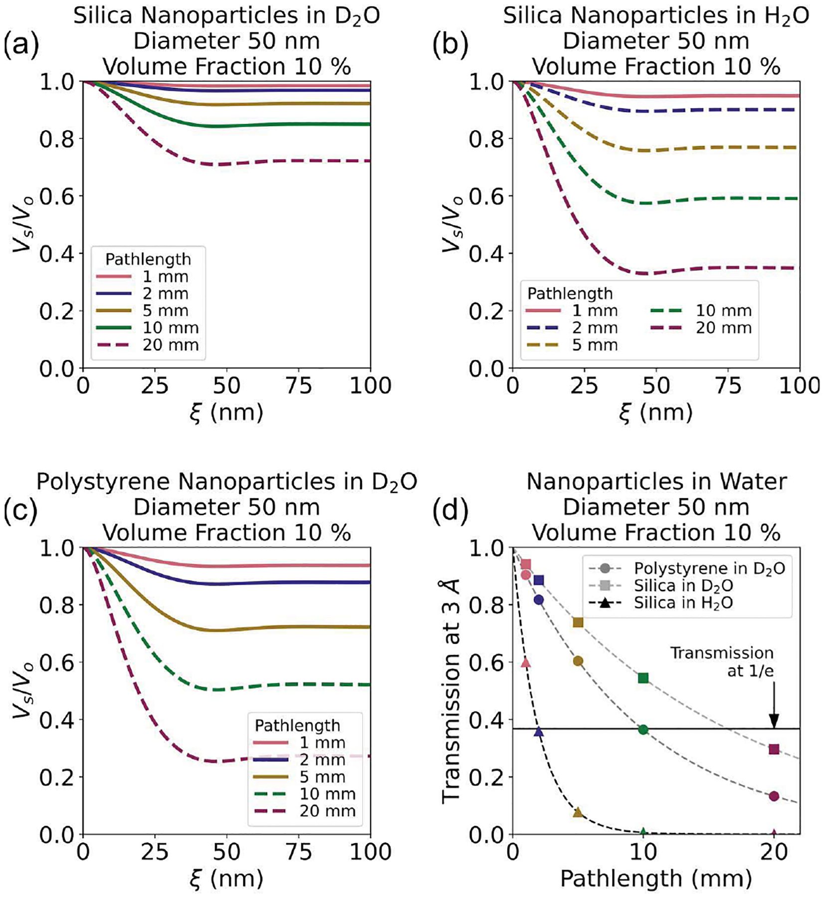
Simulated loss in visibility for (a) and (b) silica and (c) polystyrene nanoparticle dispersions in water at varying sample path lengths. All particles were modeled with a sphere form factor and hard-sphere structure factor. Dashed lines indicate path lengths that result in a transmission below the recommended 1/e limit. (d) Simulated transmission for the same nanoparticle dispersions as a function of sample path length (dashed lines). Markers and their colors match specific path lengths modeled in (a)–(c). The horizontal solid line represents the rule-of-thumb 1/e limit for transmission.
Figure 7.
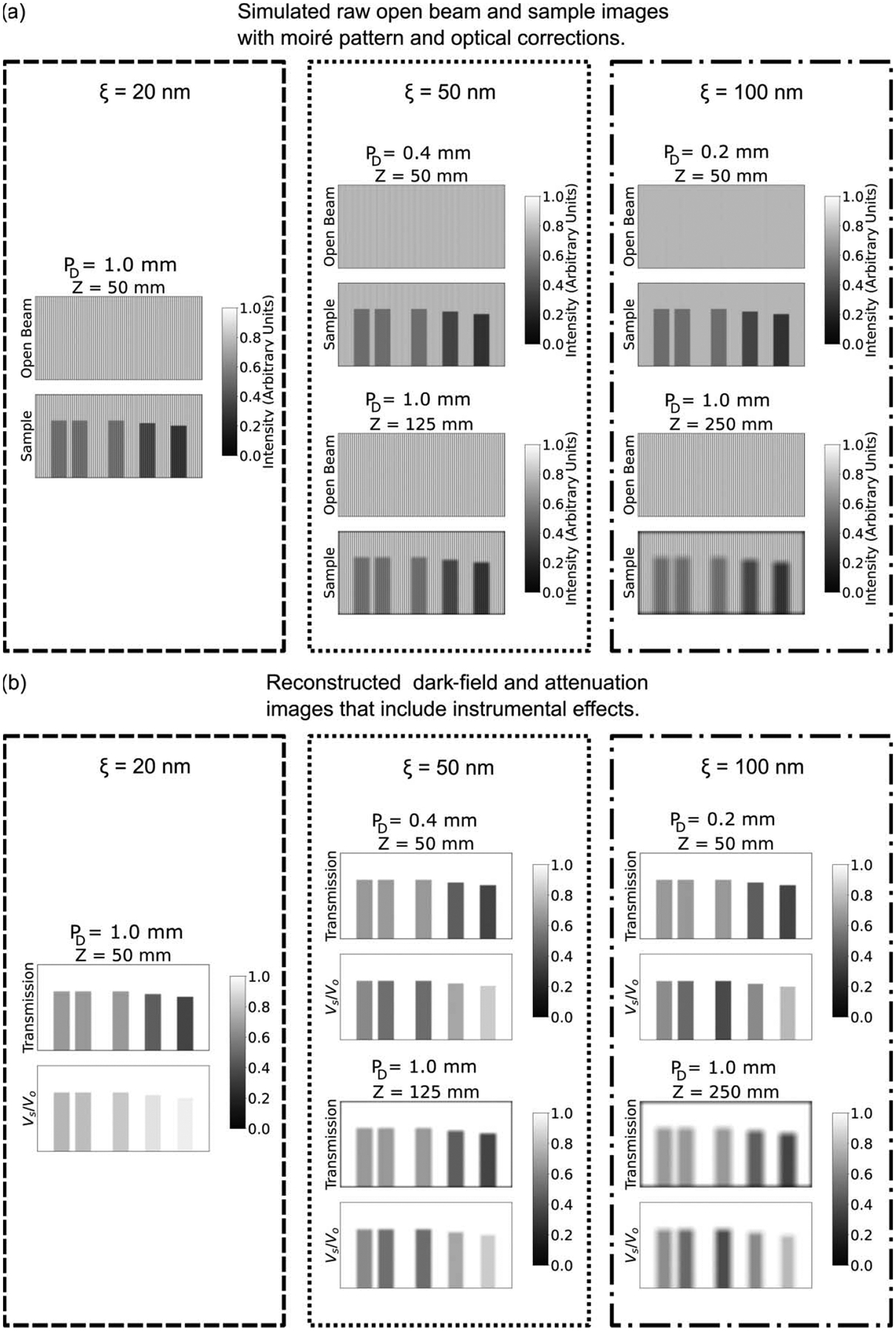
(a) Simulated raw open beam and sample images for five different unique measurement points at three autocorrelation lengths at varying sample-to-detector distances (Z) and moiré periods. (b) Corresponding reconstructed simulated neutron dark-field and attenuation images at the sample measurement conditions. Note that aliasing may cause visual distortion of the moiré pattern in the figure.
In SANS, changes in wavelength impact the q measured for a given scattering angle, the probability of a neutron scattering at a given q and the transmission of neutrons through the sample. As dark-field neutron imaging is an indirect measurement of small-angle scattering, the wavelength has the same impact on accessible autocorrelation lengths, loss in visibility and transmission. In Fig. 4 we explore this for wavelengths between 2 Å and 8 Å using an example system of 500 nm-diameter polystyrene nanoparticles suspended in D2O in a cell with a 1 mm path length (see Table S1 of the supporting information for model information). In this example, the dark-field signal increases with wavelength until 8 Å, where a complete loss in visibility is reached and the particle size is not resolvable. Due to the increased signal strength, selecting a longer wavelength may improve the measurement sensitivity to inherently weak materials with smaller microstructures. However, this simultaneously shifts the window of accessible autocorrelation lengths to longer length scales for a given moiré period and sample-to-detector distance. Moreover, the open beam visibility of each moiré period varies with wavelength (Wen et al., 2008), and thus even in monochromatic measurements, there are additional constraints on the wavelength to achieve optimal measurement conditions. Finally, these results provide insight into the smearing effects of polychromatic neutron sources in neutron dark-field imaging. Like resolution smearing in SANS, a polychromatic beam will result in a distribution of autocorrelation lengths convoluted into a single image acquisition, smoothing out features in the one-dimensional data (Barker & Pedersen, 1995). Therefore, both wavelength effects need to be carefully considered and corrected for during a measurement.
There are also parallels between SANS and dark-field neutron imaging data as a function of sample composition. This is shown in Fig. 5 for concentration, size and shape variations in polystyrene nanoparticle dispersions in heavy water with a source wavelength of 3 Å (see Tables S2 and S3 of the supporting information for model information). As the concentration increases from a volume fraction of 1% to 20% in Figs. 5(a) and 5(b), the scattering intensity and loss in visibility both increase and show the emergence of a structure factor peak capturing the interactions of neighboring particles. Harti et al. (2017) and Krouglov et al. (2003) provide detailed discussions of this transition and consistent results of the structure factor captured by both dark-field imaging and SESANS, respectively. The dark-field data have an advantage when compared with SANS as multiple scattering is easily accounted for in the path length term of equation (4), as described by Rekveldt et al. (2002). In SANS data, multiple scattering is more challenging to model (Jensen & Barker, 2018). This broadens the use cases for dark-field imaging to materials and concentrations previously classified as ‘too strong’ or infeasible for SANS or USANS (Rehm et al., 2013). In Figs. 5(c) and 5(d) the particle size is increased from 25 to 1000 nm. In both datasets, the particle size is characterized by the major slope change at the transition from smaller to larger length scales. This appears as a shoulder in the SANS data and an inverted shoulder shape in the dark-field data. Finally, Figs. 5(e) and 5(f) show simulated datasets for polystyrene nanoparticles that vary in shape, including a sphere, cube, ellipsoid and cylinder. Across both simulated SANS and dark-field datasets are slope changes at length scales related to the dimensionality of the object. Though these features may seem subtle, these results show a sensitivity of both SANS and dark-field imaging to a range of microstructural shapes.
Figure 5.
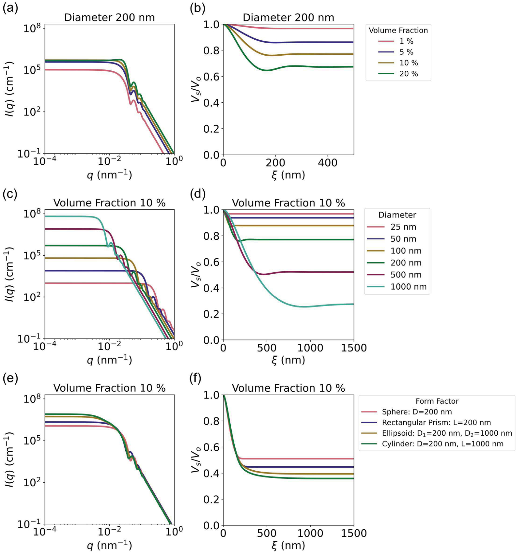
(a), (c), (e) Simulated SANS and (b), (d), (f) loss in visibility data for polystyrene nanoparticle dispersions in water. Samples vary in (a)–(b) concentration, (c)–(d) size and (e)–(f) shape. Polystyrene nanoparticles were modeled with a sphere form factor and hard-sphere structure factor.
In SANS, increasing the sample cell path length increases the scattering intensity but comes at the cost of lower transmission and increased probability of multiple scattering. The same holds true for dark-field neutron imaging apart from the previously discussed advantages of handling multiple scattering directly with an integral over the beam path through the sample. We demonstrate the effects of path length on both loss in visibility and transmission through the sample in Fig. 6 for nanoparticle dispersions of silica [Figs. 6(a) and 6(b)] and polystyrene [Fig. 6(c)] in water (see Table S4 of the supporting information for all model parameters). Here, the largest contrast is between heavy water and polystyrene (|Δρ| = 4.93 × 10⁻⁶ Å−2), followed by silica in water (|Δρ| = 4.43 × 10⁻⁶ Å−2) and silica in heavy water (|Δρ| = 2.47 × 10⁻⁶ Å−2). Though these differences may seem subtle, scattering intensity scales with Δρ2. Moreover, this is not the only factor as H1 has a much higher incoherent scattering cross-section than H2 and therefore higher concentrations of H1 lead to a strong decrease in neutron transmission through the sample. This is illustrated in Figs. 6(a) and 6(b), where the modeled dark-field signal from the silica in H2O is much larger than D2O as a function of path length, but the transmission shown in Fig. 6(d) for silica in H2O quickly drops below the rule-of-thumb 1/e transmission limit at a path length of approximately 2 mm. Meanwhile, the nanoparticle solutions in heavy water remain above this limit until path lengths between 10 mm and 20 mm. Note that these transmission values were estimated using the penetration depth calculated by the periodictable Python package, which only uses the elements’ nuclear properties as discussed in the package documentation (Kienzle, 2021). Nevertheless, they provide useful first estimates of reasonable sample configurations for dark-field imaging.
The ability to determine sample feasibility extends beyond examination of the one-dimensional loss in visibility and transmission. One must also consider noise introduced during the measurement, especially for weaker-scattering samples, and the optical effects that may limit spatial resolution. The simulated images in Fig. 7 expand on the example discussed in Fig. 2 and demonstrate the effects of noise and optical corrections on the two-dimensional data. In Fig. 7(a), simulated raw open beam and sample images are generated at three autocorrelation lengths by varying either the moiré period (top pairs) or the sample-to-detector distance (bottom pairs). Magnification and additional blurring are introduced as the sample is moved further from the detector. This limits the spatial resolution available in the reconstructed images, which are shown in Fig. 7(b) under these same measurement conditions. Significant blur is observed in both the reconstructed attenuation and the dark-field images. Additionally, the reconstructed images show an increasingly ‘grainy’ texture at smaller moiré periods as it becomes increasingly difficult to accurately characterize the sinusoidal pattern above the noise. Beyond the question of sample feasibility, these simulated images can supplement training sets for advanced segmentation models that will be required for efficient analysis of correlograms in two-dimensional and eventually three-dimensional space. Simulated measurements can be designed in such a way as to target specific performance and limitation questions of the model, e.g. at what resolution can the model effectively segment different microstructures? Or how sensitive is the model to changes in either concentration or particle size of the sample?
4. Conclusions and outlook
The Python-based package correlogram-tools builds on small-angle scattering models and the numerical Hankel transform available in SasView, and adds interferometry-relevant measurement conditions, sample compositions and configuration, and instrumental geometry to model realistic neutron dark-field spectra and generate simulated neutron dark-field and attenuation images. The ability to simulate realistic correlograms and compare directly with small-angle scattering data fosters a deeper understanding of which features in different materials and microstructures (e.g. concentration, particle size, shape) can be captured with one or both of these measurement modes, and the limits to the landscape of feasible samples. As for SANS, increases to either concentration or size result in an enhancement of the loss in visibility. Multiple scattering is also accounted for directly in dark-field neutron imaging via an integral of the beam path through the sample, giving it an advantage over traditional small-angle scattering measurements of ‘strong scatterers’. This reduces the complication of preparing some classes of samples, including geological specimens. Our exploration has also demonstrated the parallels between these two measurements. For example, while the slope changes related to specific length scales or dimensionality of the material are subtle in the spectra, both methods are sensitive to these changes. The addition of wavelength and sample path length in these simulated spectra is important for estimating a realistic dark-field signal and determining whether the system is measurable. Increases to either parameter can be used to improve the loss in visibility, but one must balance the costs of shifting the window of accessible autocorrelation lengths, signal saturation (complete loss in visibility) and lower transmission.
Simulated raw and reconstructed neutron dark-field and attenuation images provide an additional benefit to sample optimization and experimental planning. The correlogram-tools package uses the instrument geometry, such as available gratings, sample-to-detector distance, interferometer length and detector resolution, to incorporate noise and optical corrections into the simulated images, such as magnification and blur. This information is helpful to understanding the sensitivity of our instrument’s configuration, i.e. is a 5% loss in visibility measurable above the noise? Additionally, the generation of realistic image data provides a helpful alternative approach to the training of AI models for segmentation and analysis of the large stream of dark-field data expected from these measurements. Though the amount of data is too large to enable efficient analysis through more traditional manual approaches, i.e. manual model fitting, the experimental data remain insufficient for training segmentation models. Ongoing work is exploring the use of physics-based synthetic data generation as an approach to AI model training.
Finally, we note ongoing and future improvements to correlogram-tools. These include integration of a fitting functionality of correlograms extracted directly from neutron dark-field image stacks as a function of autocorrelation length. Although fitting of SESANS data is already implemented in SasView, it requires prior extraction of one-dimensional correlograms, limiting our ability to interactively explore our sample via images. The correlogram-tools package will also expand to include resolution functions for polychromatic beams that account for smearing effects on the dark-field data from the distribution of wavelengths. Additional systematics and instrument effects such as dark current, scattering from air and hydrogen, hot or dead pixels, and detector efficiency are not yet implemented in correlogram-tools but can be added in future work for more complete realistic simulated images. Up to this point, we have only discussed the simulation of dark-field imaging data in the context of two-dimensional or radiography measurements. However, dark-field imaging can be extended to three-dimensional space via tomography as described by Harti et al. (2020). The signal from microstructures contained per voxel will need to be balanced with the overall transmission through our material and the integration over multiple microstructures across the beam path rather than the single structures discussed above. Future work will expand correlogram-tools to simulations of the two-dimensional projections in such an experiment. This will be helpful to understanding this balance on a larger scale in continued sample optimization and experimental planning.
Supplementary Material
Funding information
This work was supported by National Institute of Standards and Technology (NIST) funding. Certain commercial equipment or software are identified in this paper to foster understanding. Such identification does not imply recommendation or endorsement by NIST, nor does it imply that the equipment or software identified are necessarily the best available for these purposes.
Footnotes
Supporting information: this article has supporting information at journals.iucr.org/j
References
- Allen AJ, Thomas JJ & Jennings HM (2007). Nat. Mater 6, 311–316. [DOI] [PubMed] [Google Scholar]
- Andersson R, van Heijkamp LF, de Schepper IM & Bouwman WG (2008). J. Appl. Cryst 41, 868–885. [Google Scholar]
- Bacak M, Valsecchi J,Čapek J, Polatidis E, Kaestner A, Arabi-Hashemi A, Kruk I, Leinenbach C, Long AM, Tremsin A, Vogel SC, Watkins EB & Strobl M (2020). Mater. Des 195, 109009. [Google Scholar]
- Bahadur J, Melnichenko YB, Mastalerz M, Furmann A & Clarkson CR (2014). Energy Fuels, 28, 6336–6344. [Google Scholar]
- Bakker JH, Washington AL, Parnell SR, van Well AA, Pappas C & Bouwman WG (2020). J. Neutron Res 22, 57–70. [Google Scholar]
- Barker JG & Pedersen JS (1995). J. Appl. Cryst 28, 105–114. [Google Scholar]
- Brooks AJ, Ge J, Kirka MM, Dehoff RR, Bilheux HZ, Kardjilov N, Manke I & Butler LG (2017). Prog Addit Manuf. 2, 125–132. [Google Scholar]
- Brooks AJ, Hussey DS, Yao H, Haghshenas A, Yuan J, LaManna JM, Jacobson DL, Lowery CG, Kardjilov N, Guo S, Khonsari MM & Butler LG (2018). Mater. Des 140, 420–430.. [Google Scholar]
- Busi M, Shen J, Bacak M, Zdora MC,Čapek J, Valsecchi J & Strobl M (2023). Sci. Rep 13, 15274. [DOI] [PMC free article] [PubMed] [Google Scholar]
- Doucet M, Cho JH, Alina G, Attala Z, Bakker J, Bouwman W, Bourne R, Butler P, Cadwallader-Jones I, Campbell K, Cooper-Benun T, Durniak C, Forster L, Gilbert P, Gonzalez M, Heenan R, Jackson A, King S, Kienzle P, Krzywon J, Maranville B, Murphy R, Nielsen T, O’Driscoll L, Potrze-bowski W, Prescott S, Ferraz Leal R, Rozyczko P, Snow T, Washington A & Wolf C (2022). SasView. Version 5.0.5 10.5281/ZENODO.6331344. [DOI]
- Han H, Kallakuri S, Yao Y, Williamson CB, Nevers DR, Savitzky BH, Skye RS, Xu M, Voznyy O, Dshemuchadse J, Kourkoutis LF, Weinstein SJ, Hanrath T & Robinson RD (2022). Nat. Mater 21, 518–525. [DOI] [PubMed] [Google Scholar]
- Harti RP, Strobl M, Betz B, Jefimovs K, Kagias M & Grünzweig C (2017). Sci. Rep 7, 44588. [DOI] [PMC free article] [PubMed] [Google Scholar]
- Harti RP, Strobl M, Valsecchi J, Hovind J & Grünzweig C (2020). Sci. Rep 10, 1002. [DOI] [PMC free article] [PubMed] [Google Scholar]
- Harti RP, Valsecchi J, Trtik P, Mannes D, Carminati C, Strobl M, Plomp J, Duif CP & Grünzweig C (2018). Sci Rep, 8, 17845. [DOI] [PMC free article] [PubMed] [Google Scholar]
- Huang W, Restrepo D, Jung J, Su FY, Liu Z, Ritchie RO, McKittrick J, Zavattieri P & Kisailus D (2019). Adv. Mater 31, 1901561. [DOI] [PubMed] [Google Scholar]
- Jeffries CM, Ilavsky J, Martel A, Hinrichs S, Meyer A, Pedersen JS, Sokolova AV & Svergun DI (2021). Nat. Rev. Methods Primers, 1, 70. [Google Scholar]
- Jensen GV & Barker JG (2018). J. Appl. Cryst 51, 1455–1466. [DOI] [PMC free article] [PubMed] [Google Scholar]
- Kienzle P (2021). Extensible Periodic Table, https://periodictable.readthedocs.io/en/latest/.
- Kim Y, Kim D, Hussey DS, Kim J, Mirzaei M, Pushin DA, Clark CW & Lee SW (2022). Sci. Rep 12, 3461. [DOI] [PMC free article] [PubMed] [Google Scholar]
- Kim Y, Valsecchi J, Kim J, Lee SW & Strobl M (2019). Sci. Rep 9, 18973. [DOI] [PMC free article] [PubMed] [Google Scholar]
- Kim Y, Valsecchi J, Oh O, Kim J, Lee SW, Boue F, Lutton E, Busi M, Garvey C & Strobl M (2022). Appl. Sci 12, 833. [Google Scholar]
- Kim Y, Wolf CM, Sathe PS, Daugherty MC, Robinson SM, Kienzle PA, Bajcsy P, LaManna JM, Jacobson DL, Baltic E, Weigandt KM, Murphy RP, Klimov NN, Huber MG & Hussey DS (2023). J. Phys. Conf. Ser 2605, 012015. [Google Scholar]
- Krouglov T, Bouwman WG, Plomp J, Rekveldt MT, Vroege GJ, Petukhov AV & Thies-Weesie DME (2003). J. Appl. Cryst 36, 1417–1423. [Google Scholar]
- Kupwade-Patil K, Bumajdad A, Littrell KC & Büyüköztürk O (2020). Constr. Build. Mater 243, 118175. [Google Scholar]
- Marathe S, Assoufid L, Xiao X, Ham K, Johnson WW & Butler LG (2014). Rev. Sci. Instrum 85, 013704. [DOI] [PubMed] [Google Scholar]
- Nie Z, Parai R, Cai C, Michaelis C, LaManna JM, Hussey DS, Jacobson DL, Ghosh D & Koenig GM (2021). J. Electrochem. Soc 168, 060550. [Google Scholar]
- Pfeiffer F, Grünzweig C, Bunk O, Frei G, Lehmann E & David C (2006). Phys. Rev. Lett 96, 215505. [DOI] [PubMed] [Google Scholar]
- Rehm C, Barker J, Bouwman WG & Pynn R (2013). J. Appl. Cryst 46, 354–364. [Google Scholar]
- Rekveldt M. Th., Bouwman WG, Kraan WH, Uca O, Grigoriev SV & Kreuger R (2002). Neutron Spin Echo Spectroscopy, pp. 100–115. Berlin, Heidelberg: Springer. [Google Scholar]
- Strobl M (2015). Sci. Rep 4, 7243. [DOI] [PMC free article] [PubMed] [Google Scholar]
- Strobl M, Betz B, Harti RP, Hilger A, Kardjilov N, Manke I & Gruenzweig C (2016). J. Appl. Cryst 49, 569–573. [Google Scholar]
- Strobl M, Grünzweig C, Hilger A, Manke I, Kardjilov N, David C & Pfeiffer F (2008). Phys. Rev. Lett 101, 123902. [DOI] [PubMed] [Google Scholar]
- Strobl M, Harti R, Gruenzweig C, Woracek R & Plomp J (2017). J. Imaging, 3, 64. [Google Scholar]
- Tan C, Zou J, Li S, Jamshidi P, Abena A, Forsey A, Moat RJ, Essa K, Wang M, Zhou K & Attallah MM (2021). Int. J. Mach. Tools Manuf 167, 103764. [Google Scholar]
- Valsecchi J, Kim Y, Lee SW, Saito K, Grünzweig C & Strobl M (2021). Sci. Rep 11, 8023. [DOI] [PMC free article] [PubMed] [Google Scholar]
- Valsecchi J, Strobl M, Harti RP, Carminati C, Trtik P, Kaestner A, Grünzweig C, Wang Z, Jefimovs K & Kagias M (2020). Commun. Phys 3, 42. [Google Scholar]
- Wang H-W, Anovitz LM, Burg A, Cole DR, Allard LF, Jackson AJ, Stack AG & Rother G (2013). Geochim. Cosmochim. Acta, 121, 339–362. [Google Scholar]
- Weigandt KM, Pozzo DC & Porcar L (2009). Soft Matter, 5, 4321. [Google Scholar]
- Wen H, Bennett EE, Hegedus MM & Carroll SC (2008). IEEE Trans. Med. Imaging, 27, 997–1002. [DOI] [PMC free article] [PubMed] [Google Scholar]
- White JM & Calabrese MA (2022). Colloids Surf. A Physicochem. Eng. Asp 638, 128246. [DOI] [PMC free article] [PubMed] [Google Scholar]
- Wolf CM, Kim Y, Kienzle PA, Sathe PS, Daugherty MC, Bajcsy P, Hussey DS & Weigandt KM (2023). correlogram-tools 0.1.0, https://github.com/usnistgov/correlogram_tools/tree/v0.1.0.
- Xu J, Wu H-C, Zhu C, Ehrlich A, Shaw L, Nikolka M, Wang S, Molina-Lopez F, Gu X, Luo S, Zhou D, Kim Y-H, Wang GN, Gu K, Feig VR, Chen S, Kim Y, Katsumata T, Zheng Y-Q, Yan H, Chung JW, Lopez J, Murmann B & Bao Z (2019). Nat. Mater 18, 594–601. [DOI] [PubMed] [Google Scholar]
- Yashiro W, Terui Y, Kawabata K & Momose A (2010). Opt. Express, 18, 16890. [DOI] [PubMed] [Google Scholar]
Associated Data
This section collects any data citations, data availability statements, or supplementary materials included in this article.


