AdaBoost model for rockburst intensity prediction considering class differences and quantitative characterization of misclassification difference

Abstract

With the resource development gradually into the deep, rock explosion phenomenon is more and more frequent. The suddenness and harmfulness of rockbursts threaten the safe development of underground resources. In order to more accurately predict the possible intensities of rockbursts in specific rock conditions and stress environments, the rock mechanical and stress parameters between different intensities of rockbursts are further explored, an AdaBoost model considering the differences in the hierarchy is established, and a Flash Hill-Climbing method is proposed to optimize the hyperparameters in the classification model. Finally, a misclassification difference index (MCDI) is defined to quantitatively characterize the severity of misclassification. The results show that the accuracy of the Improved AdaBoost model is about 2.3% higher than that of the Normal AdaBoost model, and the Misclassification Difference Index (MCDI) of the Normal AdaBoost model is 05, while the the Improved AdaBoost model is 00. The model can provide a theoretical reference for rockburst prediction.

Introduction

Rockbursts are generally defined as the sudden release of strain energy stored in the rock following an excavation disturbance, causing the rock to break apart and eject fragments¹. The suddenness, hazardous nature, and unpredictability of rockbursts make them a major hazard that hinders the development of deep mining.

Domestic and international research on the impact and control of rockburst tendency to use theoretical analysis, indoor and outdoor tests and numerical simulation and other methods. Fu Y et al.¹ conducted uniaxial compression tests on coal samples to investigate the effect of different filling holes on the strength and deformation resistance of the coal body.Zhao Tongbin et al.² investigated the energy release characteristics of different fracture mechanisms in rocks by means of acoustic emission signals from the test output.Song Shikang et al.³ also utilised the acoustic emission principle to study crack extension and fracture patterns in brittle coal. It can be seen that the experiments focus more on specific qualitative descriptions to achieve predictive control of rockbursts from a mechanistic point of view.

Unlike the above mentioned, Li J. et al.⁴ used the coupled method of similar simulation test and discrete element simulation to study the destructive deformation process of coal seam roof.Deng Daixin et al.⁵ established an integrated monitoring system covering the process of rockfall and obtained synergistic features that can be used as precursor information for rockbursts.Tan Yunliang et al.⁶ constructed a model with key control parameters to investigate the link between residual coal pillars and rock damage instability during multi-seam mining. Liu Tingting et al.⁷ established a numerical model of biaxial Hopkinson rod test system by using the coupled finite element method-discrete element model to study the dynamic mechanical properties and damage characteristics of intersecting jointed rock bodies with different joint distributions under peripheral pressure.Zhenyu Han et al.⁸ developed a series of discrete element models to investigate the effect of orifice shape on dynamic mechanical properties and crack evolution. Numerical simulation methods can be more intuitive through the software to simulate the process of energy aggregation, transfer and release of rock damage, and then predict the rock explosion, but due to the difficulty of describing the complex non-homogeneous nature of the rock, which limits the reliability of its prediction. Exploring more efficient and accurate rock explosion prediction methods is an important way to develop technology to control rock explosion disasters.

Single-learner prediction, integrated-learner prediction, and deep-learning algorithms have proliferated in recent years, providing a data-driven means for rockburst prediction⁹. Man Singh Basnet et al.¹⁰ proposed that rockburst prediction is categorized into long-term prediction and short-term prediction. Long-term prediction relies on environmental factors such as the magnitude of ground stress, rock properties, etc., to determine the probability of rock bursts and the intensity of rock bursts at the beginning of the excavation; Short-term predictions to determine the probability and intensity of rockbursts are based on microseismic monitoring data, etc. In a comparison of the two types, long-term predictions are slightly more fruitful. Ghasemi et al.¹¹ used C5.0 decision tree to develop two predictive models, one to predict rockburst occurrence and the other to predict rockburst intensity. The results of the study showed an accuracy of 91.1% for intensity prediction and 89.29% for probability of occurrence prediction. Li et al.¹² and Xue et al.¹³ used an extreme learning machine to predict rockburst intensity and adopted an intelligent optimization algorithm to quickly find the optimal hyperparameters to achieve favorable prediction accuracies of 80.87% and 97%, respectively. The former was predicted using three parameters: rock brittleness coefficient (BCF), rock stress coefficient (SCF) and strain energy storage index; the latter was predicted using a total of six indices: uniaxial compressive strength (UCS), uniaxial tensile strength (UTS) and minimum tangential stress (MTS) in addition to the three indices mentioned above. Li et al.¹⁴ considered seven parameters affecting rockburst destruction and, in conjunction with the rock engineering systems paradigm and neural networks, proposed a Rockburst Damage Scale Index (RDSI) for rockburst assessment, achieving an accuracy of 71% across 24 test cases. Xie et al.¹⁵ used an XGBoost model based on genetic algorithm optimization to study the effect of different numbers of indicators on prediction accuracy, and the results showed that the best combination of indicators was to use all six indicators. Ma et al.¹⁶ and Xu et al.¹⁷ used a feature selection algorithm to pre-process rockburst data to create feature variables for rockburst prediction. Probabilistic neural networks and random forest models, both with over 90% accuracy, were used to predict the processed data. Sun et al.¹⁸ used an oversampling technique to balance the dataset, followed by the generation of new data features using a polynomial feature function to filter the most important features based on a data dimensionality reduction algorithm. Finally, multiple prediction algorithms were used to make predictions. The results show that the accuracy of the dataset processed by data structure appears to be somewhat improved. Li et al.¹⁹ established four Naive Bayes statistical learning models with preset prior distributions for the assessment of rockburst hazards, and the results show that the Bayes statistical learning model based on Gaussian prior has the strongest performance.

All of the above studies used a single prediction model for prediction, and a large number of studies have shown that integrated prediction models tend to have better fitting accuracies. Xue et al.6 used Particle Swarm Optimization (PSO) to optimize the input weight matrices and hidden layer deviations of the ELM, using all six parameters for training. The model was then tested on a set of 15 typical rockburst cases from a hydropower plant on the Yangtze River in China, and showed superior performance. Saha et al.²⁰ developed a classification model combining a deep learning neural network (DLNN) and a support vector machine (SVM) for rockburst prediction and compared the results with those of individual model predictions. The results demonstrated that the integrated model outperformed the individual models, achieving an accuracy of 91.44%. Cui et al.²¹ employed a stacking integration strategy, wherein three models-gradient boosting decision tree (GBDT), bagging tree, and XGBoost-were utilized in the initial layer. The second layer employed a GBDT model to learn the outputs derived from the initial layer, subsequently generating the final decision. This decision was then combined with the group intelligent optimisation algorithm to optimize the relevant hyperparameters. The results demonstrate that the model is capable of achieving high levels of prediction accuracy. Li et al.²² and Yan et al.²³ employed a stacking integrated SVM model to classify and predict rock bursts, with the objective of identifying the optimal hyperparameters. To this end, Grid Search and K-fold cross-validation were employed to ascertain the most effective parameters. Lyu et al.²⁴ developed an integrated classifier for two-layer support vector machines, which uses feature engineering to classify the collected data parameters into two groups, which are separately classified using SVM, and finally the classification results are synthesised to obtain the classification results. Wang et al.²⁵ proposed a layer-by-layer stacking model of AK-LS-SVM classifiers embedded with transfer learning, where the output of the previous layer of classifiers is used as the input of the next layer of classifiers, thus continuously refining more abstract data. Li et al.²⁶ used three combination strategies of voting, packing and stacking to combine multiple integrated tree models and compared them with single integrated tree models. The results show that the best accuracy of a single integrated tree is 85.71%, while the model that combines XGBoost, ET and Random Forest (RF) by voting achieves the best accuracy of 88.89%. Qiu et al.²⁷ used sandcat swarm optimisation and extreme gradient boosting to predict the damage level of rockbursts with a prediction accuracy of 88.46%. R. and M. et al.²⁸ improved the updating rule of the sample weights for the cost-sensitive boosting algorithm proposed by Wang, so that the distance of each misclassified point relative to the center of its own group determines different weight values. The results showed that the strategy achieved better results.

Arsalan et al.²⁹ used numerical modelling in the Abaqus software environment to generate 300 datasets to show the effect of faults on the rockburst phenomenon in tunnels, and the results showed that the risk of rockbursts is greatly increased if the location and strike of faults around deep tunnels cause high stresses. The commonly used rockburst prediction models are summarised in Table 1.

Table 1.

Common rockburst prediction models.

Construction method	Model source	Accuracy rate/%
C5.0 decision tree	Ghasemi et al.11	89.29
extreme learning machine	Li et al.12 and Xue et al.13	80.87
Probabilistic neural networks	Ma et al.16	90
Random forest models	Xu et al.17	90
DLNN/SVM	Saha et al.20	91.44
Single integrated tree	Li et al.26	85.71
XGBoost/ET/RF	Li et al.26	88.89
sandcat swarm optimisation /extreme gradient boosting	Qiu et al.27	88.46
RF/GBDT/XGB/PCC	Zhang et al.30	75.08
AdaBoost	Ma Ke31	93.8
t-SNE/ K-means clustering/XGBoost	Ullah Barkat et al. 32	89
APSO/SVM	Li Yuefeng et al.33	95
C4.5 decision tree algorithm	Wang Yanbin et al.34	71.43

In summary, integrated classification models have attracted a lot of attention in recent years due to their higher accuracy and wider applicability, and their potential is being fully exploited. For the rockburst prediction problem, the label of the rockburst implies the level difference, and this information is often ignored. Therefore, an AdaBoost model that takes into account the misclassification difference is developed to classify rockburst data. A quantitative evaluation metric is proposed to characterize the misclassification difference of the model, providing a new methodological approach to rockburst prediction.

Previous machine learning models on the rockburst domain had no special treatment when performing weight updates for different misclassification results. Thus the machine learning domain of predicting rockburst intensity does not define the degree of misclassification. However, in actual predictions, different misclassification bring different levels of error. The same treatment of different classifications affects the accuracy of rockburst predictions. Therefore, this paper designs Improved AdaBoost model based on Normal AdaBoost model considering different error severity and proposes misclassification difference index (MCDI) to measure the severity of misclassification.

In Sect. 2, Data Information is presented, which contains information about the data source, classification and included data; Sect. 3 develops an optimisation algorithm and proposes the fundamentals of Improved AdaBoost model; Sect. 4 is showing and comparing the prediction results and the importance of the index; In Sect. 5 misclassification difference index (MCDI) is proposed in order to measure the misclassification and this is used to analyse the three prediction models; Sect. 6 is conclusion.

Data information

In this paper, the data for the rockburst intensity prediction study originate from 240 datasets of rockburst data shared by Xie et al. Some data are showed in Table 2. The data set contains six metrics to measure the probability of rockburst intensity: minimum tangential stress (MTS), uniaxial compressive strength (UCS), uniaxial tensile strength (UTS), stress ratio (SCF), brittleness coefficient (BCF) and elastic energy index (Wet).

Table 2.

Partial rockburst data.

No	Project	MTS	UCS	UTS	SCF	BCF	Wet	Rockburst Intensity	Rockburst Code
1	Diversion Tunnels of Yuzixi Hydropower Station	90	170	11.3	0.53	15.04	9.00	Moderate	3.00
2	2# Sub Tunnel of Ertan Hydropower Station	90	220	7.4	0.41	29.73	7.3	Light	2.00
3	Underground Cavern of Taipingyi Hydropower Station	62.6	165	9.4	0.38	17.53	9.00	Light	2.00
4	Underground powerhouse of Laxiwa Hydropower Station	55.40	176.00	7.30	0.32	24.11	9.30	Moderate	3.00
5	Diversion Tunnels of Tianshengqiao -II Hydropower Station	30.00	88.70	3.70	0.34	23.97	6.60	Moderate	3.00
6	Underground Powerhouse of Nor-wegian Sima Hydropower Station	48.75	180.00	8.30	0.27	21.69	5.00	Moderate	3.00
7	Diversion Tunnels of Swedish VietasHydropower Station	80.00	180.00	6.70	0.44	26.87	5.50	Light	2.00
8	Japanese Guanyue Tunnel	89.00	236.00	8.30	0.38	28.43	5.00	Moderate	3.00
9	Diversion Tunnels of Jingping Hydropower Station	98.60	120.00	6.50	0.82	18.46	3.80	Moderate	3.00
10	Italian Raibl Lead Zinc Sulfide Working	108.40	140.00	8.00	0.77	17.50	5.00	Strong	4.00
11	Soviet Rasvumchorr Workings	57.00	180.00	8.30	0.32	21.69	5.00	Moderate	3.00
……
240	Cooling Diversion Tunnels of Swedish Forsmark Nuclear Power Station	50.00	130.00	6.00	0.38	21.67	5.00	Moderate	3.00

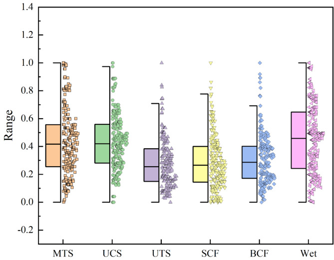
The data size distribution range of each indicator is not consistent. In order to analyse the distribution of the data and to facilitate subsequent forecasting, each indicator is normalised separately. The distribution of the indicator data after normalisation is presented in Fig. 1.

Fig. 1.

Distribution of indicator data.

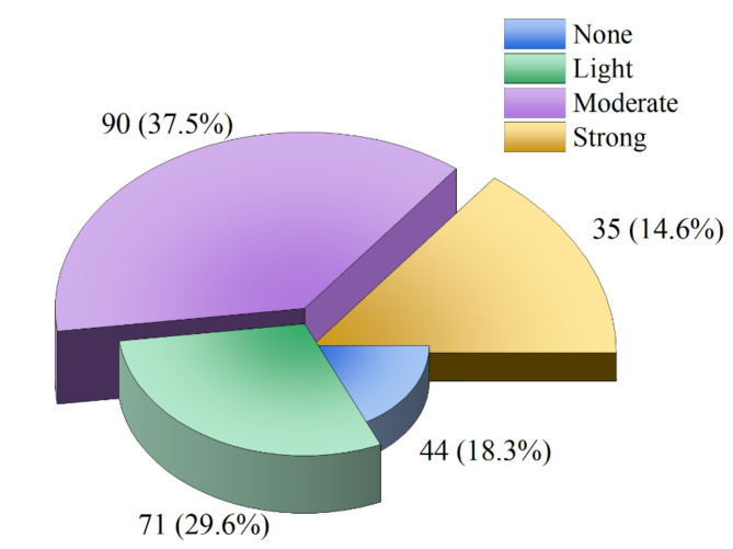
In addition to the indicator data, the dataset contains a set of labels, namely rock burst intensity. The rockburst intensities were classified into four levels: None, Light, Moderate and Strong. The number and percentage of each rockburst intensity are shown in Fig. 2.

Fig. 2.

Data intensity classification percentage chart.

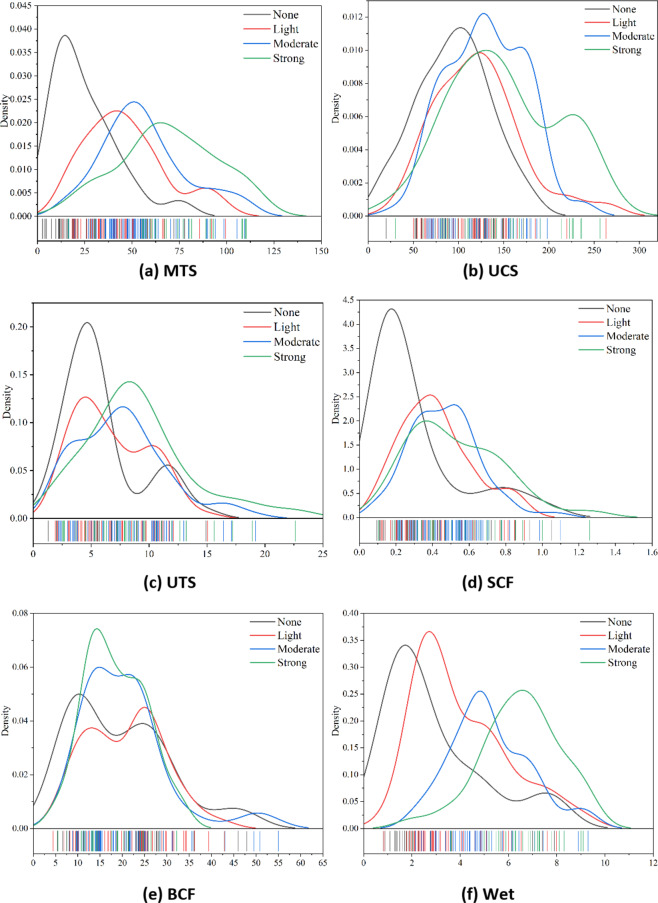
The varying intensities of rockbursts are contingent upon the disparate ranges of data distributions observed across the six indicators previously outlined, in addition to the interactions between them. As illustrated in Fig. 3, the distribution of the data pertaining to the six indicators across each intensity label for rock bursts. The horizontal axis represents the range of data sizes for this indicator, while the vertical axis represents the corresponding number density at a fixed value for a given category. As illustrated in the figure, MTS and W_et are able to distinguish between all four categories of rockburst intensity. UCS and SCF exhibit a clear characterisation of the no-rockburst scenario, while there is no clear differentiation between the other three categories. UTS can divide the dataset into two categories, one consisting of no rockbursts and minor rockbursts, and the other consisting of moderate rockbursts and intense rockbursts; whereas BCF does not make a clear distinction between the four categories.

Fig. 3.

Distribution of data for different indicators.

The principle and construction of the model

Flash Hill-climbing method

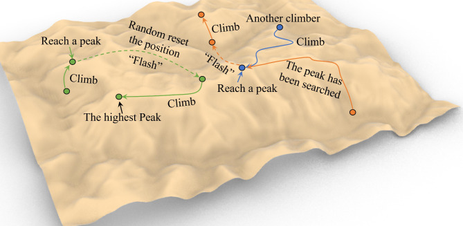
The Hill-Climbing algorithm is an efficient optimisation algorithm that calculates the height of each “climber” in front of, behind and to the right of the climber in order to guide the climber to the summit of the mountain. The algorithm is straightforward and efficacious, although it does present a significant challenge: it tends to adhere to each mountain, making it difficult to identify the highest peak in the region. Upon reaching the summit of a mountain, the climber’s position is reset, initiating a new climb. This process greatly enhances the probability of identifying the highest peak, akin to a constantly blinking indicator. To prevent the re-climbing process from becoming circular, it is necessary to create a map that records the status of all paths across the entire map. Only when a location has not yet been explored should it be selected as a potential landing spot for the next step. In this manner, by ascending and repositioning themselves, climbers can traverse as many routes as possible, thereby exploring the largest possible area and thus identifying the highest peak. The deployment of multiple climbers in concert enables the identification of the optimal position with greater efficiency.

The improved climbing algorithm possesses three key points:

①A climbing rule that only goes higher up;

②Reset its position when there is no way to climb;

③A map that saves all the position states.

The algorithm works as shown in Fig. 4. The flow of the algorithm is shown in Table 3.

Fig. 4.

Schematic of Flash Hill-Climbing algorithm.

Table 3.

Flash Hill-climbing algorithm.

Flash Hill-Climbing algorithm
1. Initialise multiple climbers positions x1, y1 = random(X, Y); x2, y2 = random(X, Y);…; xn, yn =random(X, Y) 2. Find locations around each point that can be moved: if G(temp_x, temp_y) = = 0 and 0 ≤ temp_x ≤ X and 0 ≤ temp_y ≤ Y 3. Calculate the highest position among the movable points around the climber and move over it
xn, yn = arg max(f(xn, yn), f(temp_x, temp_y)) G(xn, yn) = 1 4. If there are no moving points in the vicinity, or if there are no higher points, the position of the point is reset. xn, yn = random(X, Y) and G(xn, yn) = = 0 5. Repeat 2 ~ 4 steps to a certain number of steps or to reach the set accuracy

In the table X, Y represent the search range, random (X, Y) means to generate a set of random numbers in the range of (X, Y), and G is a map that records the search status of all points in the range. The function f (x, y) is a fitness function, or an accuracy function, if it is set to an error rate function, the algorithm needs to be changed to a downward walk. By constantly climbing and constantly blinking, it is possible to walk over every peak in the range as far as possible.

Improvement of weight update algorithm for AdaBoost model

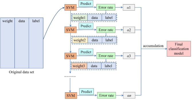
The AdaBoost (Adaptive Boosting) model is an integrated learning method that consists of a more powerful strong classifier, created by integrating multiple weak classifiers. The weak classifier h1(x) is initially trained using samples with equal sample weights. Based on the classification results of the weak classifier h1(x), the misclassified samples are given higher weights, while the correctly classified samples are given lower weights. This process draws attention to the misclassified samples at the next classifier h1(x), and a more specific classifier is subsequently trained. A weight is assigned to each classifier based on its error rate, indicating the importance of this classifier in determining the final classification result. Repeating these steps, multiple classifiers are trained, and these classifiers are accumulated according to the weights of the previously obtained classifiers to obtain the final desired strong classifier, as shown in the principle in Fig. 5.

Fig. 5.

Principle of AdaBoost model.

However, the traditional AdaBoost model treats any misclassification result equally. During the process of updating the weights, only the determination of whether the current sample is correctly classified is made, while the degree of misclassification is not defined. However, in rockburst intensity prediction, the degree of absurdity brought by the misclassification of None category into Light category and misclassification into Strong category is not the same, which can cause serious misclassification of the real situation. Consequently, greater consideration should be given to this significant misclassification when sample weight updates are conducted, in order to ensure that the necessary attention is drawn to this issue.

The formula for calculating the weights of each subclassifier in the AdaBoost algorithm is:

\documentclass[12pt]{minimal} \usepackage{amsmath} \usepackage{wasysym} \usepackage{amsfonts} \usepackage{amssymb} \usepackage{amsbsy} \usepackage{mathrsfs} \usepackage{upgreek} \setlength{\oddsidemargin}{-69pt} \begin{document}$${\alpha _m}=\log \left( {\frac{{1 - {e_m}}}{{{e_m}}}+\log \left( {L - 1} \right)} \right)$$\end{document} 1

Where L is the number of categories and e_m is the training error of the m-th classifier on the training set, which is calculated as:

\documentclass[12pt]{minimal} \usepackage{amsmath} \usepackage{wasysym} \usepackage{amsfonts} \usepackage{amssymb} \usepackage{amsbsy} \usepackage{mathrsfs} \usepackage{upgreek} \setlength{\oddsidemargin}{-69pt} \begin{document}$${e_m}=\sum\limits_{{i=1}}^{N} {{w_{mi}}sign\left( {{{\hat {y}}_i} \ne {y_i}} \right)}$$\end{document} 2

Where N is the number of samples, \documentclass[12pt]{minimal} \usepackage{amsmath} \usepackage{wasysym} \usepackage{amsfonts} \usepackage{amssymb} \usepackage{amsbsy} \usepackage{mathrsfs} \usepackage{upgreek} \setlength{\oddsidemargin}{-69pt} \begin{document}$${\hat {y}_i}$$\end{document} is the predicted value of the i-th sample and is the true value of the i-th sample, \documentclass[12pt]{minimal} \usepackage{amsmath} \usepackage{wasysym} \usepackage{amsfonts} \usepackage{amssymb} \usepackage{amsbsy} \usepackage{mathrsfs} \usepackage{upgreek} \setlength{\oddsidemargin}{-69pt} \begin{document}$$sign\left( {{{\hat {y}}_i} \ne {y_i}} \right)$$\end{document} generates True or False, i.e. a value of 0 or 1, based on the judgement result. \documentclass[12pt]{minimal} \usepackage{amsmath} \usepackage{wasysym} \usepackage{amsfonts} \usepackage{amssymb} \usepackage{amsbsy} \usepackage{mathrsfs} \usepackage{upgreek} \setlength{\oddsidemargin}{-69pt} \begin{document}$${w_{mi}}$$\end{document} is the weight corresponding to the i-th sample on the m-th classifier. The update formula for the weights is:

\documentclass[12pt]{minimal} \usepackage{amsmath} \usepackage{wasysym} \usepackage{amsfonts} \usepackage{amssymb} \usepackage{amsbsy} \usepackage{mathrsfs} \usepackage{upgreek} \setlength{\oddsidemargin}{-69pt} \begin{document}$${w_{m+1,i}}={w_{m,i}}{e^{{\alpha _m}{w_{m,i}}sign\left( {{{\hat {y}}_i} \ne {y_i}} \right)}}$$\end{document} 3

The weight update formula above is the way commonly used in multi-classification tasks and the way implemented in the sklearn library. However, this update method does not treat each misclassification type differently, as described above. The samples with the worst misclassification type are given a higher weight to reflect their absurdity. Therefore, some changes are made to Eq. 3:

\documentclass[12pt]{minimal} \usepackage{amsmath} \usepackage{wasysym} \usepackage{amsfonts} \usepackage{amssymb} \usepackage{amsbsy} \usepackage{mathrsfs} \usepackage{upgreek} \setlength{\oddsidemargin}{-69pt} \begin{document}$${w_{m+1,i}}=\frac{{{w_{m,i}}}}{{{Z_m}}}{e^{{\alpha _m}{w_{m,i}}\sqrt {{{\left( {{{\hat {y}}_i} - {y_i}} \right)}^2}} }}$$\end{document} 4

The formula \documentclass[12pt]{minimal} \usepackage{amsmath} \usepackage{wasysym} \usepackage{amsfonts} \usepackage{amssymb} \usepackage{amsbsy} \usepackage{mathrsfs} \usepackage{upgreek} \setlength{\oddsidemargin}{-69pt} \begin{document}$${Z_m}=\sum\limits_{{i=1}}^{N} {{w_{m,i}}}$$\end{document} serves to keep the sum of the weights equal to 1. The Euclidean distance is used to define the gap between two categories, and ensures both the positive qualitative nature of the results. The differences between the categories are sufficiently differentiated by the Eq. 4.

The construction of AdaBoost models

AdaBoost is an integrated model consisting of several identical weak classifiers combined. Improved AdaBoost (IAB) and Normal AdaBoost (NAB) models are built, consisting of 10 SVM models, where the sample weight formula for IAB is defined by Eq. 4 and the sample weight formula for NAB is the standard form, (i.e. Equation 3). Meanwhile, to compare the effect of the integrated model, another SVM model is built to perform the same training and classification tasks. Five metrics, MTS, W_et, UCS, SCF and UTS are used in the dataset.

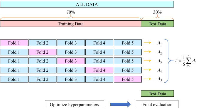
The hyperparameters of the IAB, NAB and SVM models are C and γ. The number of classifiers of the integrated model is fixed to 10, and all the internal weak classifiers use the same hyperparameters. The two parameters are optimised using the proposed Flash Hill-Climbing algorithm, and the 5-fold cross-validation results are used as the target accuracy, as shown in Fig. 6.

Fig. 6.

5-fold cross-validation schematic.

The comparison of forecast results and model features

The comparison of model predictions

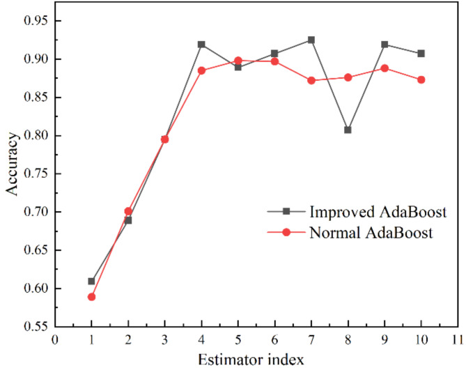
In order to perform the model training, both IAB and NAB use a combination of 10 SVMs. The accuracies achieved by the respective training sets of the 10 classifiers are presented in Fig. 7. As illustrated in the Fig. 7, the initial classifiers exhibit a relatively low degree of accuracy, with the accuracy of subsequent classifiers reaching a level of approximately 90% as the weights of misclassified samples continue to increase. When considered collectively, the accuracy of the classifiers within the NAB is slightly inferior to that of the IAB. The suggests that the improvements to the weighting formulae have a positive impact.

Fig. 7.

Comparison of the prediction accuracy of individual classifiers in the IAB model and the NAB model.

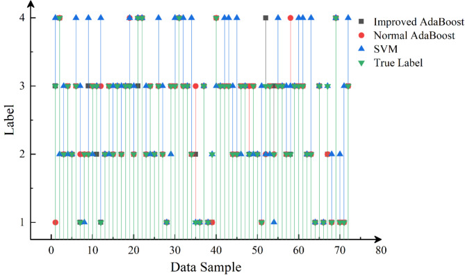
Figure 8 illustrates the performance of IAB, NAB and SVM on the test samples. When the sign of the model is in alignment with the true label, it can be inferred that the sample has been correctly predicted. Table 4 presents the statistical analysis of the accuracy of each model on the test set. From the figure and table, it can be seen that IAB performs slightly better than NAB, and SVM performs generally on the test set, which is a limitation of the weak classifier itself. Therefore, the integrated classifier can effectively improve the classification accuracy. And the accuracy is also improved, after updating the sample weight formula for rockburst data which has a level difference of labels.

Fig. 8.

Performance of IAB, NAB and SVM on test samples.

Table 4.

Correctness of each model on the test set.

Model	Correct Number	Error Number	Accuracy
Improved AdaBoost	64	8	88.9%
Normal AdaBoost	62	10	86.1%
SVM	41	31	56.9%

The comparison of model features

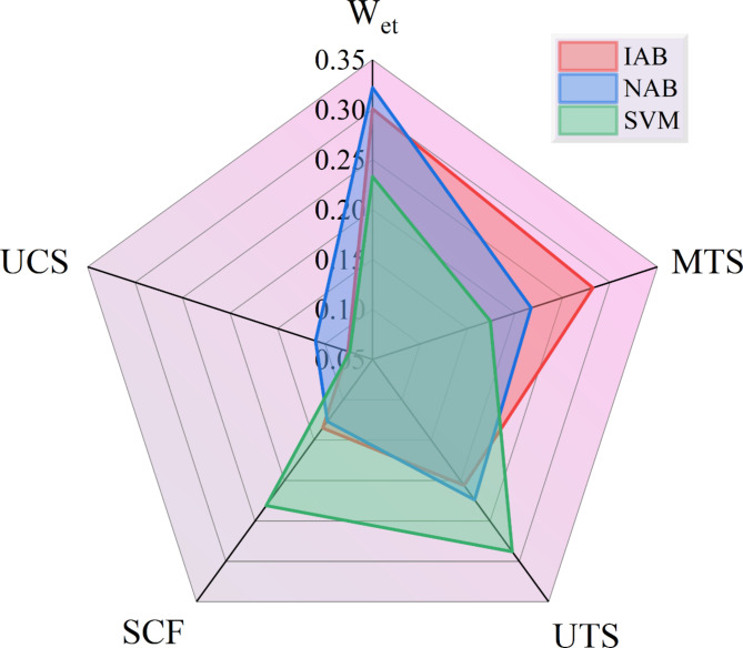
The radar chart of feature importance for IAB, NAB and SVM is shown in Fig. 9. From the figure it can be seen that for IAB the most important metric is W_et followed by MTS with importance values of 0.301 and 0.282 respectively.For NAB the importance level of Wet and UTS is higher with values of 0.322 and 0.224 respectively.The SVM model has a higher degree of importance for UTS at 0.288, followed by Wet with a value of 0.233, which is significantly different from the other two models.The UCS indicator simultaneously possesses the lowest importance in all three models.The order of importance of IAB and NAB is also in line with the findings of the previous data distribution information.The higher importance of UTS and SCF in SVM may be misleadingly related to the high density of data without rockbursts.

Fig. 9.

Radar chart of the importance of the five indicators.

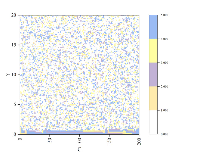
Figure 10 illustrates the path diagrams of the five points in Flash Hill-Climbing algorithm. From the figure, it can be observed that the five points have a large number of continuous paths in the lower region, while in the middle region they are all just intermittent steps, indicating that in the middle region there are just some bumpy hills. The paths travelled by the 5 points are evenly spread throughout the region, enabling the search for each peak as far as possible, which effectively avoids locally optimal solutions and thus searches for globally optimal solutions. This method is comparatively straightforward and efficacious in comparison to other optimisation algorithms. Upon examining the color coverage area, it can be postulated that extending the search in a downward direction may prove to be a more fruitful endeavor. Nevertheless, the outcomes of numerous experiments have indicated that continuing the search downward will likely result in a significant degree of overfitting.

Fig. 10.

Path diagram of 5 points in the scintillating mountaineering algorithm.

Indicators of the degree of variation in projected results

Construction of indicators of the degree of variability of the projected results

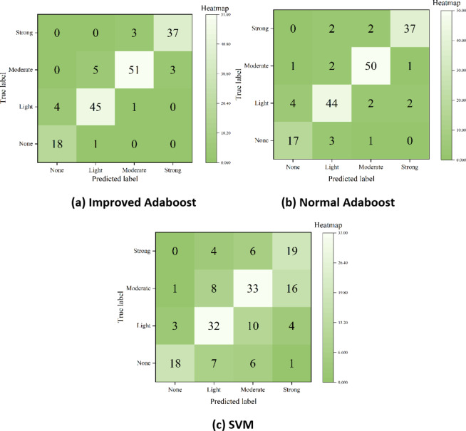
The confusion matrix is a frequently employed tool for illustrating the precision of the classification outcomes. The confusion matrices for IAB, NAB, and SVM model are presented in Fig. 11, and Table 5 displays the corresponding accuracies for these three models. In order to provide a more detailed description of the misclassification difference, it is defined that when the predicted label and the true label are separated by x labels, it is defined (x + 1)-order classification error. By analogy, the misclassification of a None label as a Strong label is referred to as the third-order classification error. Similarly, the correctly classified case can be referred to as the 0-order classification error. From the data in Table 5, it can be found that the classification accuracy of IAB has slightly increased. From the Fig. 11, the IAB misclassifies samples close to the diagonal and produces only first-order classification errors; second-order classification errors occur in both the NAB and the SVM model; third-order classification errors occur only in the SVM model.

Fig. 11.

Classification error plots for the three models.

Table 5.

Accuracy of the training set.

Model	Correct Number	Error Number	Accuracy
Improved AdaBoost	151	17	89.8%
Normal AdaBoost	148	20	88.1%
SVM	102	66	60.7%

In order to quantitatively measure the degree of misclassification variance, it is necessary to define a misclassification difference index (MCDI) in the form of a sum of squares.

\documentclass[12pt]{minimal} \usepackage{amsmath} \usepackage{wasysym} \usepackage{amsfonts} \usepackage{amssymb} \usepackage{amsbsy} \usepackage{mathrsfs} \usepackage{upgreek} \setlength{\oddsidemargin}{-69pt} \begin{document}$$MCDI=\frac{1}{N}\sum\limits_{{i=1}}^{N} {{{\left( {\hat {y} - y} \right)}^2}}$$\end{document} 5

As in Eq. 5, the squared form is employed to artificially widen the gap between classes. In the event of a first-order classification errors, the MCDI is equal to 1. In the case of a second-order classification errors, the MCDI widens to a factor of 4. In the most extreme case, where a third-order classification errors has been produced, a factor of 9-times gap is produced. However, in terms of the consequences of classification errors, it is important to note that a single serious classification error does not equate to numerous minor errors. If thousands, or even millions, of classifications of rockburst samples were performed, the 4-times and the 9-times difference would be rapidly diluted by the sample size. Consequently, this method of defining the metric is not sufficiently robust.

A developed misclassification difference index

As illustrated in Fig. 12, the numbers in the black circles represent the 0-th order classification errors, designated as DL0, the orange circles represent the first-order classification errors, designated as DL1, and so on. The primary objective of establishing the MCDI is to quantify the proportion of second-order and third-order classification errors. The following definitions are provided:

\documentclass[12pt]{minimal} \usepackage{amsmath} \usepackage{wasysym} \usepackage{amsfonts} \usepackage{amssymb} \usepackage{amsbsy} \usepackage{mathrsfs} \usepackage{upgreek} \setlength{\oddsidemargin}{-69pt} \begin{document}$$MCDI=ceil\left( {\frac{{DL2}}{{DL1+DL2+DL3}} \times 10} \right)+ceil\left( {\frac{{DL3}}{{DL1+DL2+DL3}} \times 10} \right) \times 10$$\end{document} 6

Fig. 12.

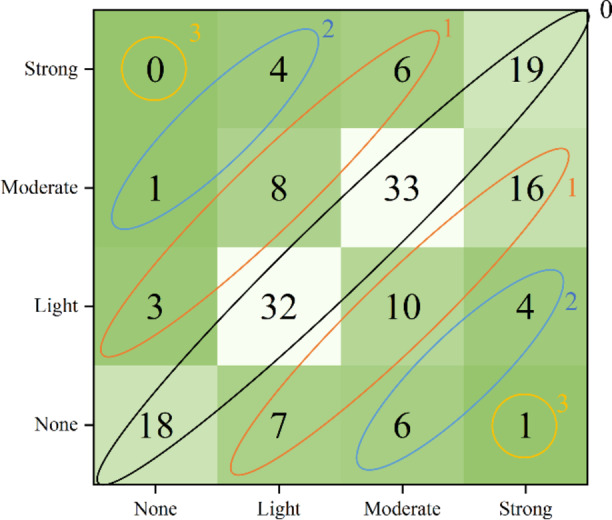
Schematic diagram of classification error.

The Equation \documentclass[12pt]{minimal} \usepackage{amsmath} \usepackage{wasysym} \usepackage{amsfonts} \usepackage{amssymb} \usepackage{amsbsy} \usepackage{mathrsfs} \usepackage{upgreek} \setlength{\oddsidemargin}{-69pt} \begin{document}$$ceil(\cdot )$$\end{document} is the upward rounding function. In general, the MCDI calculation produces a two-digit number, with the single-digit number and the ten-digit number consisting of two parts, which are separated by a plus sign on the right side of the equals sign of Eq. 6, respectively. The left part is the ratio of the second-order classification error to the total, multiplied by 10, and then rounded to produce a single-digit number. The right part is the ratio of the third-order classification error to the total, and ultimately multiplied by 10 to form the ten-digit number of the MCDI. The advantage of this approach is that there is no longer an order of magnitude equivalence between the misclassification difference. If DL2 or DL3 is 0, the corresponding value is also set to 0. However, when the percentage of DL2 or DL3 reaches 0.9 or above, this indicator is no longer effective, and it is therefore necessary to examine the classifier in order to identify the cause of the numerous classification errors that it is generating. Table 5 presents the MCDI for the IAB, NAB and SVM.

Table 6 demonstrates that the IAB does not generate second-order classification errors or third-order classification errors, whereas the SVM model produces third-order classification errors. Furthermore, the percentage of second-order classification errors is less than that of the NAB. By combining the MCDI with the accuracy rate, it is possible to gain a comprehensive understanding of the classification effect of a classifier.

Table 6.

Number of classification errors and MCDI for the three models.

Model	DL1	DL2	DL3	MCDI
Improved AdaBoost	17	0	0	00
Normal AdaBoost	14	6	0	05
SVM	50	15	1	13

Conclusions

For data such as rockbursts, where labels have obvious hierarchical relationships and level difference, a regularized weighting formula based on the AdaBoost model that takes into account the disparity of label is proposed. An optimization algorithm named Flash Hill-Climbing algorithm is used to find the optimal hyperparameters, and the results of 5-fold cross-validation are used as the objective of the optimization algorithm to avoid overfitting phenomenon as much as possible. Finally, a quantitative characterization of the misclassification difference of the model is proposed to reflect the performance effect of the classifier in level difference data. The main conclusions are as follows:

(1) A total of 240 sets of rockburst data were collected, and the percentages of rockburst cases in the four intensities were 18.3%, 29.6%, 37.5%, and 14.6%, respectively. Of the six parameters, MTS and Wet are the most effective at differentiating between the four categories of rockburst intensity; UCS and SCF distinguish between no rockbursts; UTS can distinguish between one category consisting of no rockbursts and minor rockbursts, and another category consisting of moderate rockbursts and intense rockbursts; BCF does not distinguish clearly between the four categories.

(2) The weight update formula in the AdaBoost model has been modified, and two new algorithms have been proposed: the Flash Hill-Climbing algorithm for optimising hyperparameters and the improved integrated classification model considering the level difference. The classification accuracies of the test set for the IAB, NAB, and SVM are 88.9%, 86.1%, and 56.9%, respectively. The results demonstrate the improved classification of the IAB.

(3) In order to quantitatively characterize the misclassification difference, an MCDI parameter is proposed to reflect the classification effect of the classifier on the level difference data. It consists of two digits, the first digit characterises the proportion of second-order classification error, the tenth digit characterises the proportion of third-order classification error, and there is no equivalence between the classification errors of the three levels, so that the classification effect can be independently represented.

Limitations

Compared with the results of these previous studies, our model achieves good results. However, the best results may not be achieved due to the differences in the performance of the model itself and the quality of the training data, which is also our future work plan.

Author contributions

Yunzhen Zhang is responsible for data collection, code writing and article writing, Guangquan Zhang is responsible for providing ideas and writing guidance, Tengda Huang is responsible for article revision, Yuxin Liu is responsible for part of the code writing, and Nanyan Hu is responsible for the article image processing.

Data availability

Data is provided within the manuscript.

Declarations

Competing interests

The authors declare no competing interests.

References

- 1.Fu, Y. et al. Mechanical properties and energy evolutions of burst-prone coal samples with holes and fillings. Int. J. Coal Sci. Technol.11, 40 (2024). [Google Scholar]
- 2.Zhao, T. et al. Master crack types and typical acoustic emission characteristics during rock failure. Int. J. Coal Sci. Technol.10, 2 (2023). [Google Scholar]
- 3.Song, S. et al. Fracture features of brittle coal under uniaxial and cyclic compression loads. Int. J. Coal Sci. Technol.10, 9 (2023). [Google Scholar]
- 4.Li, J., Zhang, M., Wang, C., Liao, C. & Zhang, B. Failure characteristics and fracture mechanism of overburden rock induced by mining: A case study in China. Int. J. Coal Sci. Technol.11, 44 (2024). [Google Scholar]
- 5.Deng, D., Wang, H., Xie, L., Wang, Z. & Song, J. Experimental study on the interrelation of multiple mechanical parameters in overburden rock caving process during coal mining in longwall panel. Int. J. Coal Sci. Technol.10, 47 (2023). [Google Scholar]
- 6.Tan, Y. et al. Study on the disaster caused by the linkage failure of the residual coal pillar and rock stratum during multiple coal seam mining: Mechanism of progressive and dynamic failure. Int. J. Coal Sci. Technol.10, 45 (2023). [Google Scholar]
- 7.Liu, T. et al. Three-dimensional numerical simulation of dynamic strength and failure mode of a rock mass with cross joints. Int. J. Coal Sci. Technol.11, 17 (2024). [Google Scholar]
- 8.Han, Z., Liu, K., Ma, J. & Li, D. Numerical simulation on the dynamic mechanical response and fracture mechanism of rocks containing a single hole. Int. J. Coal Sci. Technol.11, 64 (2024). [Google Scholar]
- 9.Askaripour, M., Saeidi, A., Rouleau, A. & Mercier-Langevin, P. Rockburst in underground excavations: A review of mechanism, classification, and prediction methods. Undergr. Space. 7, 577–607. 10.1016/j.undsp.2021.11.008 (2022). [Google Scholar]
- 10.Man Singh Basnet, P. et al. A comprehensive review of intelligent machine learning based predicting methods in long-term and short-term rock burst prediction. Tunn. Undergr. Space Technol.142, 105434. 10.1016/j.tust.2023.105434 (2023). [Google Scholar]
- 11.Ghasemi, E., Gholizadeh, H. & Adoko, A. C. Evaluation of rockburst occurrence and intensity in underground structures using decision tree approach. Eng. Comput.36, 213–225. 10.1007/s00366-018-00695-9 (2020). [Google Scholar]
- 12.Li, M., Li, K. & Qin, Q. A rockburst prediction model based on extreme learning machine with improved Harris Hawks optimization and its application. Tunn. Undergr. Space Technol.134, 104978. 10.1016/j.tust.2022.104978 (2023). [Google Scholar]
- 13.Xue, Y., Bai, C., Qiu, D., Kong, F. & Li, Z. Predicting rockburst with database using particle swarm optimization and extreme learning machine. Tunn. Undergr. Space Technol.98, 103287. 10.1016/j.tust.2020.103287 (2020). [Google Scholar]
- 14.Li, N., Naghadehi, Z., Jimenez, M. & R Evaluating short-term rock burst damage in underground mines using a systems approach. Int. J. Min. Reclam. Environ.34 (8), 531–561 (2020). [Google Scholar]
- 15.Xie, X., Jiang, W. & Guo, J. Research on rockburst prediction classification based on GA-XGB model. IEEE Access.9, 83993–84020. 10.1109/ACCESS.2021.3085745 (2021). [Google Scholar]
- 16.Ma, L., Cai, J., Dai, X. & Jia, R. Research on rockburst risk level prediction method based on LightGBM – TCN – RF. Appl. Sci.12, 8226. 10.3390/app12168226 (2022). [Google Scholar]
- 17.Xu, G., Li, K., Li, M., Qin, Q. & Yue, R. Rockburst intensity level prediction method based on FA-SSA-PNN model. Energies. 15, 5016. 10.3390/en15145016 (2022). [Google Scholar]
- 18.Sun, L. et al. Ensemble stacking rockburst prediction model based on Yeo–Johnson, K-means SMOTE, and optimal rockburst feature dimension determination. Sci. Rep.12, 15352. 10.1038/s41598-022-19669-5 (2022). [DOI] [PMC free article] [PubMed] [Google Scholar]
- 19.Li Ning, X., Jimenez., R. & Feng. Predicting Rock Burst Hazard with Incomplete Data Using Bayesian Networks. 61–70 (Tunnelling and Underground Space Technology incorporating Trenchless Technology Research, 2017).
- 20.Saha, S. et al. Novel ensemble of deep learning neural network and support vector machine for landslide susceptibility mapping in Tehri region, Garhwal Himalaya. Geocarto Int.37, 17018–17043. 10.1080/10106049.2022.2120638 (2024). [Google Scholar]
- 21.Cui, S., Yin, Y., Wang, D., Li, Z. & Wang, Y. A stacking-based ensemble learning method for earthquake casualty prediction. Appl. Soft Comput.101, 107038. 10.1016/j.asoc.2020.107038 (2021). [Google Scholar]
- 22.Li, X. et al. A novel deep stacking least squares support vector machine for rolling bearing fault diagnosis. Comput. Ind.110, 36–47. 10.1016/j.compind.2019.05.005 (2019). [Google Scholar]
- 23.Yan, T., Shen, S. L., Zhou, A. & Chen, X. Prediction of geological characteristics from shield operational parameters by integrating grid search and K-fold cross validation into stacking classification algorithm. J. Rock Mech. Geotech. Eng.14, 1292–1303. 10.1016/j.jrmge.2022.03.002 (2022). [Google Scholar]
- 24.Lyu, Y., Gong, X. & Two-Layer, A. SVM Ensemble-classifier to Predict Interface Residue Pairs of Protein Trimers. Molecules25, 4353. 10.3390/molecules25194353 (2020). [DOI] [PMC free article] [PubMed] [Google Scholar]
- 25.Wang, G., Zhang, G., Choi, K. S. & Lu, J. Deep additive least squares support Vector machines for classification with model transfer. IEEE Trans. Syst. Man. Cybern Syst.49, 1527–1540. 10.1109/TSMC.2017.2759090 (2019). [Google Scholar]
- 26.Li, D., Liu, Z., Armaghani, D. J., Xiao, P. & Zhou, J. Novel ensemble intelligence methodologies for rockburst assessment in complex and variable environments. Sci. Rep.12, 1844. 10.1038/s41598-022-05594-0 (2022). [DOI] [PMC free article] [PubMed] [Google Scholar]
- 27.Qiu, Y. & Zhou, J. Short-term rockburst damage assessment in burst-prone mines: An explainable XGBOOST hybrid model with SCSO algorithm. Rock. Mech. Rock. Eng.56, 8745–8770. 10.1007/s00603-023-03522-w (2023). [Google Scholar]
- 28.P. M., S. R. Performance enhanced boosted SVM for imbalanced datasets. Appl. Soft Comput.83, 105601. 10.1016/j.asoc.2019.105601 (2019).
- 29.Arsalan Mahmoodzadeh, N. H. et al. Numerical and Machine Learning Modeling of Hard Rock Failure Induced by Structural Planes Around Deep Tunnels (Engineering Fracture Mechanics, 2022).
- 30.Zhang, H., Xia, Y., Lin, M., Huang, J. & Yan, Y. A three-step rockburst prediction model based on data preprocessing combined with clustering and classification algorithms. Bull. Eng. Geol. Environ.83, 266 (2024). [Google Scholar]
- 31.Numerical Analysis on the Factors. Affecting the hydrodynamic performance for the parallel surfaces with microtextures. J. Tribol. 136 (1-), 021702 (2014). [Google Scholar]
- 32.Ullah, B., Kamran, M. & Rui, Y. Predictive modeling of short-term rockburst for the stability of subsurface structures using machine learning approaches: t-SNE, K-Means clustering and XGBoost. Mathematics. 10, 449 (2022). [Google Scholar]
- 33.Li, Y. et al. Rockburst prediction based on the KPCA-APSO-SVM model and its engineering application. Shock Vib. 7968730 (2021).
- 34.Wang, Y. Prediction of rockburst risk in coal mines based on a locally weighted C4.5 algorithm. IEEE Access.9, 15149–15155 (2021). [Google Scholar]
Associated Data
This section collects any data citations, data availability statements, or supplementary materials included in this article.
Data Availability Statement