Leveraging infrared spectroscopy for automated structure elucidation

Abstract

The application of machine learning models in chemistry has made remarkable strides in recent years. While analytical chemistry has received considerable interest from machine learning practitioners, its adoption into everyday use remains limited. Among the available analytical methods, Infrared (IR) spectroscopy stands out in terms of affordability, simplicity, and accessibility. However, its use has been limited to the identification of a selected few functional groups, as most peaks lie beyond human interpretation. We present a transformer model that enables chemists to leverage the complete information contained within an IR spectrum to directly predict the molecular structure. To cover a large chemical space, we pretrain the model using 634,585 simulated IR spectra and fine-tune it on 3,453 experimental spectra. Our approach achieves a top–1 accuracy of 44.4% and top–10 accuracy of 69.8% on compounds containing 6 to 13 heavy atoms. When solely predicting scaffolds, the model accurately predicts the top–1 scaffold in 84.5% and among the top–10 in 93.0% of cases.

Infrared spectroscopy stands out as an analytical tool for its affordability, simplicity, and accessibility, however, its use has been limited to the identification of a select few functional groups, as most peaks lie beyond human interpretation. Here, the authors use a transformer model that enables chemists to leverage all information contained within an IR spectrum to directly predict the molecular structure.

Introduction

Infrared (IR) spectroscopy has been widely used in chemistry since the early 1900s when a link between specific peaks in the IR spectrum and functional groups was demonstrated¹. Since then, the affordability and ease of use of IR spectrometers made them a staple in chemical laboratories, giving chemists a quick and easy way to identify which functional groups are present in a sample². Beyond the identification of functional groups, IR spectroscopy enables the identification of chemical compounds by matching their spectra to a database. This method has found applications in forensics, pharmaceuticals, and food science allowing automated structure elucidation from IR spectra^3–6.

However, the need for an exhaustive database remains a critical limitation in the effective utilisation of this technique. This is exacerbated by the complexity and overlapping nature of peaks rendering accurate annotation of the spectra difficult for chemists. While identifying specific functional groups such as the carbonyl peak around 1700 cm⁻¹ is straightforward, decoding the fingerprint region (400–1500 cm⁻¹) is a much more daunting task². Consequently, chemists have traditionally only utilised a minimal amount of the information present in an IR spectra to detect the presence of a handful of functional groups, leaving a significant portion of the spectrum’s potential for structure determination untapped.

Over the past decades, the increased availability of nuclear magnetic resonance (NMR) spectroscopy and liquid chromatography mass spectrometry (LC-MS) has diminished the role of IR spectroscopy as a structure elucidation tool in research chemistry⁷. While NMR and LC-MS provide more readily interpretable data, each has its own limitations. NMR spectroscopy necessitates deuterated solvents, costly equipment, and measurement times ranging from 10 minutes to several hours⁸. Similarly, LC-MS requires expensive high-purity solvents and extensive method development. Moreover, the sample is destroyed during the analysis and database matching is required for structure elucidation^9,10. In contrast, IR spectroscopy is quick, cost-effective, non-destructive, and easy to use. However, it too has drawbacks, primarily the need for relatively high concentrations of pure analytes, especially when compared to LC-MS.

With the rise of computing power, a wave of new statistical methods (i.e. machine and deep learning) have allowed tackling previously challenging problems such as image classification or language modelling^11,12.

Machine learning and especially transformer models have shown great promise in chemistry. Applications of such models range from predicting retrosynthetic routes, over designing novel drug candidates to aiding in the automation of experiments^13–15. In the field of IR spectroscopy, machine learning has also advanced the processing and prediction of spectra. Graph neural networks (GNNs) have been used extensively to predict the IR spectrum from molecular graphs^16–18 whereas Convolutional neural networks (CNNs) have achieved state-of-the-art performance on predicting functional groups from IR spectra^19,20. Other types of machine learning models, such as support vector machines (SVMs), random forest models, and multilayer perceptrons (MLPs), have also been employed to predict functional groups from IR spectra^21–23.

Despite the pressing need for rapid and accurate structure elucidation methods in chemistry, direct prediction of the complete chemical structure from IR spectra has yet to be accomplished, even with the recent advances in machine learning. Unlocking this capability would enable chemists to fully utilise the information present in IR spectra and breathe new life into the use of IR spectroscopy in analytical chemistry. Additionally, such a fast and cost-effective elucidation tool would have broad applicability across various fields, ranging from research chemistry over metabolomics to forensics.

Here, we present the, to the best of our knowledge first work using a machine learning model for full structure elucidation from the IR spectrum. We use a transformer model trained on both the chemical formula and the IR spectrum to directly predict the molecular structure as Simplified molecular-input line-entry system (SMILES)^24,25. We first pretrain the model on simulation IR spectra obtained using molecular dynamics and the class II polymer consistent force field (PCFF)²⁶. Then we fine-tune the model on experimental spectra from the National Institute of Standards and Technology (NIST) IR database²⁷. We evaluate the model’s ability to predict the correct molecule, scaffold and functional groups from the experimental IR spectrum. Our model achieves a 44.4% top–1 and 69.8% top–10 accuracy while predicting the correct structure, 84.5% top–1 and 93.0% accuracy to predict the scaffold and an average F1 score of 0.856 when predicting 19 functional groups.

Results and Discussion

Model

In this work we use an autoregressive encoder-decoder transformer architecture. This architecture has shown high performance in across various chemical tasks, particularly excelling at generating SMILES strings^28,29. We train the model in a sequence-to-sequence fashion providing it with an IR spectrum from which the model generates the corresponding chemical structure.

In addition to the IR spectrum we also present the model with the chemical formula as input. The chemical formula serves as a strong prior limiting the chemical space the model explores. The generated molecules are represented as SMILES (see Fig. 1).

Fig. 1. Summary of the processing and prediction pipeline.

Top: Raw spectra are obtained either from simulation or from the NIST IR database²⁷. The raw spectrum is processed and together with the chemical formula converted into the input representation. Bottom: The input representation is fed into the transformer model to predict molecular structure as SMILES.

More details on the architecture are given in the methods section.

Simulated IR spectra

In contrast to other work we use molecular dynamics to simulate IR spectra. This causes the to spectra contain features such as anharmonicities not present if the harmonic oscillator approximation was used. This renders the spectra more realistic.

We simulate a total of 634,585 IR spectra using molecular dynamics and the PCFF forcefield²⁶. The structures corresponding to the IR spectra were sampled from PubChem³⁰. We exclude charged molecules, stereoisomers, and any molecules containing atoms other than carbon, hydrogen, oxygen, nitrogen, sulphur, phosphorus, and the halogens. Furthermore, we limit the heavy atom count to a range of 6–13. A detailed description of how the data was generated can be found in the methods section and a comparison between the simulated and experiment spectra is provided in Supporting Information section 1.

Model pretraining

To optimise the model before fine-tuning on the experimental spectra, we train a total of 28 models, employing different data augmentation techniques and varying the inclusion of the chemical formula, token length, and section of the IR spectrum. For each spectrum in the test set, we generate ten ranked predictions and calculate the accuracy of each model by comparing the predicted structures to the target structure. Specifically, we report the top–1, top–5, and top–10 accuracy metrics, which indicate the percentage of cases where the predicted structure matches the target structure within the first, first five, and first ten predictions, respectively. Two molecules are defined as matching if their canonical SMILES strings match exactly. Table 1 shows the results of the trained models. In the following, we analyse the methodological choices adopted for data preparation and their respective effects. Unless otherwise specified each experiment is performed on a single fold of the data.

Table 1.

Summary of experiments on simulated data

	Formula	Spectrum	Tokens*	Window	Representation	Top–1%	Top–5%	Top–10%
Chemical formula	✓	✗	N/A	N/A	SMILES	0.01	0.03	0.06
	✗	✓	400	Full	SMILES	17.01	33.6	39.37
	✓	✓	400	Full	SMILES	26.21	51.38	59.63
Sequence length	✓	✓	100	Full	SMILES	19.17	41.21	49.63
	✓	✓	200	Full	SMILES	23.14	46.27	54.59
	✓	✓	300	Full	SMILES	25.78	50.47	58.81
	✓	✓	400	Full	SMILES	26.21	51.38	59.63
	✓	✓	500	Full	SMILES	18.03	39.67	47.26
	✓	✓	600	Full	SMILES	3.36	10.49	14.18
	✓	✓	700	Full	SMILES	2.31	7.54	10.40
	✓	✓	800	Full	SMILES	2.22	7.13	9.63
	✓	✓	900	Full	SMILES	2.13	6.71	9.01
	✓	✓	1000	Full	SMILES	2.89	9.05	12.40
Window	✓	✓	400	UM IR‡	SMILES	10.14	26.37	33.98
	✓	✓	400	Fp†	SMILES	25.83	48.39	56.36
	✓	✓	400	Full	SMILES	26.21	51.38	59.63
	✓	✓	400	Merged§	SMILES	30.22	55.87	63.88
Fingerprint: Sequence length	✓	✓	300	Fp†	SMILES	20.09	39.83	47.13
	✓	✓	400	Fp†	SMILES	25.83	48.39	56.36
	✓	✓	500	Fp†	SMILES	14.17	32.06	39.26
Merged: Sequence length	✓	✓	300	Merged§	SMILES	22.79	43.09	50.15
	✓	✓	400	Merged§	SMILES	30.22	55.87	63.88
	✓	✓	500	Merged§	SMILES	25.51	49.7	56.67
Molecular Representations	✓	✓	400	Merged§	SELFIES	5.24	14.87	19.53
	✓	✓	400	Merged§	DeepSMILES	27.03	49.97	56.95
	✓	✓	400	Merged§	SMILES	30.22	55.87	63.88
Best Augmented	✓	✓	400	Merged§	SMILES	36.43	62.49	70.00
Best Ensemble	✓	✓	400	Merged§	SMILES	45.33	72.21	78.50

* Number of tokens encoding the IR spectrum.

^† Fp: Fingerprint, 400–2000 cm⁻¹.

^‡ UM IR: Upper middle IR, 2000–3982 cm⁻¹.

^§ Merged: 400–2000 cm⁻¹ and 2800–3300 cm⁻¹.

Chemical Formula

In order to constrain the chemical space explored, we provide both the chemical formula and the IR spectrum as input to the model.

To assess the effect of this combination we train three models: one solely using the IR spectrum, another relying exclusively on the chemical formula, and a third combining both modalities (see Table 1, “Chemical Formula”). The model incorporating both the spectrum and formula as input outperforms both other models. Conversely, the model trained solely on the chemical formula performs the worst being only able to predict the correct structure in the top–10 in 0.056% of cases. This demonstrates that the model does not only provide reasonable isomers for a given chemical formula but instead is able to learn structural features from the IR spectrum.

Sequence length

The resolution of the spectrum and the degree of information available to the model are both determined by the sequence length. As the length of the sequence increases, transformer models generally exhibit a decrease in performance³¹. Therefore, we study the effect of varying the number of tokens encoding the spectra from 100 to 1000. This is equivalent to altering the resolution of the spectrum from  ~ 36 cm⁻¹ to  ~ 3.6 cm⁻¹ (see Fig. 2 and Table 1, “Sequence length”).

Fig. 2. Model accuracy plotted against the token length.

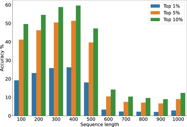
We plot the accuracy of the model (Top–1, –5, –10) against the length of the sequence encoding the IR spectrum. Performance increases up to 400 tokens before degrading sharply.

When the sequence length is increased the accuracy increases up to a maximum, followed by a sharp decrease. At low sequence lengths, the input data does not provide sufficient information to allow the model to make an informed decision. On the other hand, the model struggles with longer sequences, as with an increase in resolution a lot of the values in the spectra become redundant and the model has to differentiate between relevant and redundant information. Based on these findings, a sequence length of 400 token performs best was chosen for all further experiments. A sequence length of 400 corresponds to a spectral resolution of approximately 16 cm⁻¹. This is comparable to the typical distance between peaks in an IR spectrum. As such, models trained with a token length of 400 likely perform well because this resolution effectively discretizes the peaks in the spectrum. This discretization allows the model to capture the essential features of the spectrum without being overwhelmed by noise or excessive detail.

Window selection

Equally important as the sequence length is which part of the spectrum the model is trained on, given that some sections of the IR spectrum, e.g. the fingerprint region contain vastly more peaks than others. In all previous experiments, the model was trained on the full spectrum. Here we vary the window, i.e. the specific part of the spectrum which is provided as input. We selected four distinct sets: the full spectrum (resolution:  ~ 9 cm⁻¹), the fingerprint region (400–2000 cm⁻¹, resolution: 4 cm⁻¹), the upper middle IR region (2000–3982 cm⁻¹, resolution:  ~ 5 cm⁻¹), and a merged split containing the fingerprint region and a window in the range of 2800–3300 cm⁻¹ (resolution: 5.25 cm⁻¹). The number of tokens describing the spectrum was kept constant at 400, causing the resolution to differ from set to set.

After evaluating the performance of each window (see Table 1, “Window”), we found that the merged split performs best. On the other hand, the upper middle IR region performs the worst as this region mostly consists of hydrogen stretches and overtones. The fingerprint and the full spectrum perform similarly, indicating that the higher detail of the fingerprint region compensates for the loss of information with regards to the full spectrum. This demonstrates that the model is capable of learning the relationship between the anharmonicities of the IR fingerprint region and how they change with the molecular structure. The merged split performs best, likely because it contains both the fingerprint region and the region around 3000 cm⁻¹ while providing more detail than the full spectrum option. In addition, we perform several experiments varying the merged window. See Supporting Information section 2 for further details.

To verify that 400 tokens still yield the best performance for the two best-performing windows we carried out two experiments on the fingerprint and merged split (see Table 1, “Fingerprint: Sequence length” and “Merged: Sequence length”). For each window we trained a model with 300 and 500 tokens. In both cases the model with a sequence length of 400 performs best.

Molecular representation

As important as the representation of the IR spectra is the selection of a suitable representation for the generated molecules. While SMILES are currently most commonly used other representations such as SELFIES and DeepSMILES^32,33. We train a model on both representation and compare it to one trained on SMILES (see Table 1, Molecular Representations). While DeepSMILES perform slightly worse than SMILES, we observe a sharp drop-off in performance for SELFIES. We train all further models using SMILES.

Data augmentation

The training data was augmented using six different methods: Adding noise to the spectrum, smoothing the signal, horizontally shifting the spectrum, Extended Multiplicative Spectral Augmentation (EMSA) as proposed by Blazhko et. al.³⁴, adding an offset to the spectrum and lastly multiplying the signal with a randomly sampled vector. Each augmentation is described in further detail in the Methods. Table 2 shows the effect of each method separately and the impact on the performance of a model trained on data augmented using all methods. Each augmentation method increases the data by a factor of two.

Table 2.

Results of different augmentation techniques

	Top–1%	Top–5%	Top–10%
Vertical Noise	6.97	18.53	23.55
EMSA*	7.93	21.08	56.38
Offset	29.55	55.70	63.40
No Augmentation	30.22	55.87	63.88
Multiplication	31.96	58.07	66.09
Smoothing	35.47	61.1	68.54
Horizontal shift	36.43	62.49	70.0
Horizontal shift + Smoothing	31.82	58.11	66.17
Horizontal shift + Smoothing (augmented test set)	31.77	58.12	66.13

*Extended Multiplicative Spectral Augmentation.

The addition of noise to the signal and EMSA significantly degrade the performance of the model. We hypothesise that the addition of noise disrupts precise patterns in the shape of the peaks that the model can leverage to predict the molecular structure and thus degrades the performance. On the other hand EMSA distorts the baseline of the spectrum similarly disrupting patterns in the spectra.

Adding an offset to the spectra and multiplicative augmentation do not lead to a significant increase in performance. This is likely caused by both methods not increasing the diversity of the training set.

In contrast, both horizontal shifting and smoothing the spectrum result in a 5–6% increase in performance, with horizontal shifting showing a slight advantage over smoothing. Based on these results, a model was trained using both horizontally shifted and smoothed data. We observed that its performance was comparable to the non-augmented model. These findings prompted us to evaluate the performance of the model on augmented data to ascertain whether the model had become more adept at interpreting the augmented data. However, the evaluation on the augmented data yielded results that were similar to the non-augmented test set. Accordingly, we believe that the decreased performance results from the increased complexity found in the augmented data.

Ensembles

Ensembling is commonly used to increase the performance of machine learning models. The technique is based on combining multiple different models or multiple checkpoints of the same model and sampling from the most confident model at each prediction step. This increases performance as each model or checkpoint has a slightly different perspective on the data.

To this end we evaluate an ensemble of the five best performing checkpoints of a single training run. Another technique similar to ensembling averages the model weights of multiple checkpoint. We make use of this technique by averaging the ten best checkpoints of two different training runs and evaluate an ensemble of these two averaged checkpoints. This further increases the accuracy by 5% and 9% respectively (see Table 3).

Table 3.

Results of different ensembling techniques

	Top–1%	Top–5%	Top–10%
Augmented Model	36.43	62.49	70.00
Ensemble of 5	41.42	68.79	75.46
Ensemble of 2 avg. of 10	45.33	72.21	78.50

Fine-tuning on Experimental Data

We fine-tune the best model (augmented with horizontal shift and avg. of 10) on 3453 experimental spectra obtained from the NIST IR dataset²⁷. 721 compounds found both in the simulated and experimental data were removed from the simulated pretraining set. Experimental spectra in the training set were augmented using horizontal shift using the “Merged” window representation and 400 tokens. A summary of 5 experiments is shown in Table 4. During all experiments the training, test and validation set were kept identical and the results displayed below were obtained using the best ensembling technique as described above. Further information on the dataset can be found in the Supporting Information section 3 and 4.

Table 4.

Experiments on the NIST dataset (N = 3453 spectra)

	Start $\tilde{v}$ (cm−1)*	Top–1%	Top–5%	Top–10%
Zero Shot	400	0.09	1.89	2.48
Trained from Scratch	450	14.74	36.99	40.75
	400	44.70	68.07	70.53
Fine-Tuning	450	45.72	66.47	69.52
	550	45.33	65.50	68.33
5-fold Cross Validation	450	44.39 ± 5.31	66.85 ± 3.08	69.79 ± 2.48

*Starting wavenumber of the model.

We fine-tune the best model (augmented with horizontal shift and avg. of 10) on 3453 experimental spectra obtained from the NIST IR dataset²⁷. 721 compounds found both in the simulated and experimental data were removed from the simulated pretraining set. Experimental spectra in the training set were augmented using horizontal shift. A summary of 5 experiments is shown in Table 4. During all experiments the training, test and validation set were kept identical and the results displayed below were obtained using the best ensembling technique as described above.

All simulated data have a starting range of 400 cm⁻¹. However, 2012 of the experimental spectra cover 450–3966 cm⁻¹ while the remaining 1441 have a range of 550–3846 cm⁻¹. To use the already pretrained models with simulated data, we pad the experimental spectra i.e. filling the missing values with 0. In addition, two additional models were trained on simulated data starting at 450 cm⁻¹ and 550 cm⁻¹ respectively.

For the initial experiment, the pretrained baseline model, with a starting range of 400 cm⁻¹, was used without any modifications to predict the structure based on the spectrum (see Table 4, “Zero Shot”). Here the model performs poorly with a top–1 accuracy of just 0.09%. This outcome was expected given that the model was trained solely on simulated spectra, and highlights the substantial disparity between the simulated and experimental spectra.

Experimental infrared spectra and computed spectra obtained using force fields differ in several key aspects. Computed spectra typically neglect solvation effects which in this specific case are not relevant as the NIST dataset consists of gas-phase IR spectra. However, environmental factors, the specific instrumentation and experimental setup employed for the acquisition of IR spectra play a crucial role. The type of spectrometer, sample preparation method, and cuvette used, can impact the recorded infrared spectrum. Each instrument has its own spectral resolution, sensitivity, and calibration parameters, which contribute to the observed spectral features. Computed spectra using force fields do not consider these instrumental factors. Finally, the accuracy of the force field itself can impact the comparison between computed and experimental spectra. However, this model is performing notably better than the model trained solely on the chemical formula (see Table 1, “Chemical Formula”), demonstrating that the model is able to transfer some of the learnings from the simulated to the experimental data.

Next we trained a model from scratch solely on the experimental data. Here a starting value of 450 cm⁻¹ was employed, with spectra starting at 550 cm⁻¹ being padded with zero. Surprisingly, this model is capable of predicting the correct structure as the top–1 suggestion in 14.74% of cases. This is a testament to the models ability to learn even from a very small amount of data.

We fine-tune three different models trained on starting wavenumbers of 400, 450 and 550 cm⁻¹, respectively, on the experimental data to investigate the effect of the starting wavenumber (see Table 4, “Fine-Tuning”). All fine-tuned models significantly outperform the zero shot and trained from scratch results. The differences between the three models are minimal. In terms of the top–1 accuracy all models lie in  ~ 1% and for the top–10 accuracy within  ~ 2%. The small difference between the different models is likely a result of the limited training data (only 2477 examples augmented to 7432).

To validate the results we perform a 5-fold cross validation with a starting wavenumber of 450 cm⁻¹. We obtain a final top–1 accuracy of 44.39%, top–5 accuracy of 66.85% and top–10 accuracy of 69.79%.

Model analysis

In the following, we present an analysis of the fine-tuned model with respect to different characteristics, such as the heavy atom count or the presence of specific functional groups. The results are based on the 5-fold cross validation on experimental data.

Heavy atom dependency

To analyse the model’s performance, we evaluate its accuracy against the heavy atom count. Figure 3 shows a negative correlation between the heavy atom count (i.e. all atoms without hydrogen of a molecule) and the accuracy. In addition to the the fine-tuned model, the performance on simulated data is shown as a dashed line. On average, the top–1 accuracy of the model is  ~10% worse on experimental than on simulated data. This discrepancy can be attributed to two factors: the limited number of available experimental spectra and the simulated spectra having less noise and greater consistency compared to their experimental counterparts. The similar accuracy reported above is a result of the different heavy atom count distributions between the two sets with the average heavy atom being 9.64 for the experimental set and 11.50 for the simulated one. See Supporting Information Section 5 for the heavy atom distribution of the simulated and experimental dataset.

Fig. 3. Heavy atom count vs accuracy.

Experimental results are shown as solid lines and results on simulated data as dashed lines. A negative correlation is observed for both curves.

The negative correlation of the model’s performance with the heavy atom count likely stems from three factors. Firstly, as the heavy atom count increases, molecules become more complex, resulting in longer SMILES strings. Since the model predicts molecules autoregressively, even a single incorrectly predicted token can produce a significantly different structure. Secondly, structural features that influence molecule vibrations increase non-linearly with molecule size. As a result, the spectrum becomes denser, leading to peak overlap and diminishing the model’s predictive capability. Additionally, the increasing heavy atom count exponentially expands the chemical space, resulting in a greater number of potential isomers that the model has to differentiate, making the prediction more challenging. However, all three factors can be mitigated by augmenting the model’s training data. By incorporating more data and skewing the heavy atom distribution in the training set towards larger molecules, the model can learn to better discriminate crowded spectra, differentiate diverse isomers, and enhance overall performance. Moreover, an increased data volume would also allow for a larger model architecture with potential performance improvements.

Functional group to structure

Another factor affecting the model’s performance is the nature of the functional groups. We evaluated the model’s ability to predict the correct molecular structure based on the presence of a set of 19 functional groups in the target molecule (see Fig. 4). The functional group definitions and results in tabular form can be found in Section 6 of the Supporting Information with detailed results outlined in section 7. To avoid bias caused by the size of the underlying compounds, we calculated the average heavy atom count for molecules containing each of the particular groups. The average heavy atom count for all functional groups falls within 9.8 ± 0.8.

Fig. 4. Model accuracy plotted against the occurrence of specific functional group in the target molecule.

Top–1%, Top–5% and Top–10% performance are shown in blue, orange and green respectively.

The model performs best when fluorine, bromine or iodine are present in the target molecule. This is likely a result of these functional groups being present in the chemical formula simplifying the prediction task for the model.

On the other hand, the model performs poorly when predicting the structure of tertiary and secondary amines. This can likely be attributed to the very similar peaks exhibited by both functional groups. The low performance of both groups is further investigated below.

Functional group prediction

Previous research has focused on predicting functional groups from the IR spectrum^19–21. To compare our work in this common task we assessed the model’s performance by comparing the functional groups present in the target molecule with those in the top–1 prediction (see Fig. 5). All halogens were excluded from this analysis as their presence in the chemical formula makes the prediction trivial. The model demonstrates high accuracy in predicting the presence of most functional groups, with F1 scores above 0.8 for all functional groups except secondary amines, cyano-groups and amides (see Section 8 in the Supporting Information). Overall, the model has an average F1 score of 0.856 and an average weighted F1 score of 0.902 on the functional groups analysed. The model’s poor performance on predicting secondary amines can be attributed to two factors. Firstly the peaks of secondary amines are very similar to those of tertiary amines and secondly the training examples for tertiary amines outweigh those for secondary amines by a factor of  ~2.6. For the other four functional groups with an F1 score below 0.83, cyano, amide, sulphide and aldehyde, the low performance can be explained by each occurring fewer than 100 times in the experimental dataset.

Fig. 5. Functional group accuracy.

The model’s ability to predict the correct functional group in the target molecule. Calculated by comparing the functional groups of the top–1 prediction to the ground truth.

It is interesting to observe that while our model was trained to predict molecular structure, it achieves a high accuracy predicting functional groups, even being competitive with models trained solely to perform this task. Jung et al. achieved a weighted F1 score of 0.930 using CNNs²⁰ while Fine et al. demonstrated an average F1 score of 0.926 using MLPs²¹. To keep the results consistent we adopted the exact functional group definitions used in each paper for the following comparison. However, when comparing to Jung et al. a total of 18 functional groups were removed from the set either because there was no molecule with that particular functional group in our dataset (9 groups) or because there were less than 15 examples in the dataset (9 additional groups). Our model is competitive with both of these previous results (see Table 5) outperforming Jung et al. It is important to highlight that our model was trained with half the data in case of Fine et al. and a magnitude less data in case of Jung et al. More experimental data would likely lead to an increase in the performance of the model. On the other hand the datasets used to train and evaluate each of the models is different, leading to the functional group distributions being different as well. This complicates the comparison between different models.

Table 5.

Functional Group Predictions

Functional group definition	Model	Training Set	Avg. F1	Avg. Weighted F1
Jung (37 groups)20	Jung20	50.936	0.850	0.930
	Ours	3.453	0.864	0.945
Fine (15 groups)21	Fine21	7.393	0.926	N/A.
	Ours	3.453	0.882	0.946

Functional group heat map

To assess why the model makes wrong predictions, we analyse the correlation between the expected functional group and the incorrectly predicted functional group. For this we analyse the set of predictions where the expected functional group is not present in the top–1 prediction (see Fig. 6). We calculate the representation of functional groups in the set of false positives for a given functional group compared to the normal distribution of the test set (see Section 9 in the Supporting Information). In the heat map, if a functional group has a value of six, it represents that it occurs six times more frequently in the set of target molecules where a wrong prediction was made compared to the whole test set. In contract, a value below zero indicates an underrepresentation, while a value of zero signifies that the distribution is equivalent in both the set of incorrect predictions and the entire test set.

Fig. 6. Heatmap of the over/under-representation of functional groups.

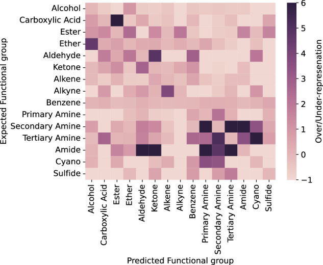
The darker the hue the more over-represented a specific functional group is.

The heatmap in Fig. 6 shows high values where there is a strong correlation between the expected and predicted functional group, i.e. when the model confuses certain functional groups. Interestingly, the model’s confusion patterns align with what one might expect from a human interpreting an IR spectrum. For example, the model often confuses carboxylic acids with esters, which is expected given the similarity of their peaks in the 1700 cm⁻¹ region. Similarly the model confuses ethers with alcohols and amides with aldehydes and ketones. To explain the models low performance at predicting secondary amines we analyse what functional groups the model confuses them with. For secondary amines, these functional groups are mostly amides and primary and tertiary amines. This behaviour can be explained by all four functional groups absorbing in the 1200–1350 cm⁻¹ range.

Similarity

The Tanimoto similarity³⁵ to the ground truth was calculated for all predicted molecules, excluding correct predictions. A histogram of the similarities is depicted in Fig. 7. The mean similarity for the whole set is 0.487. This value represents a relatively high similarity, demonstrating the model’s general understanding of IR spectra.

Fig. 7. Tanimoto similarity distribution.

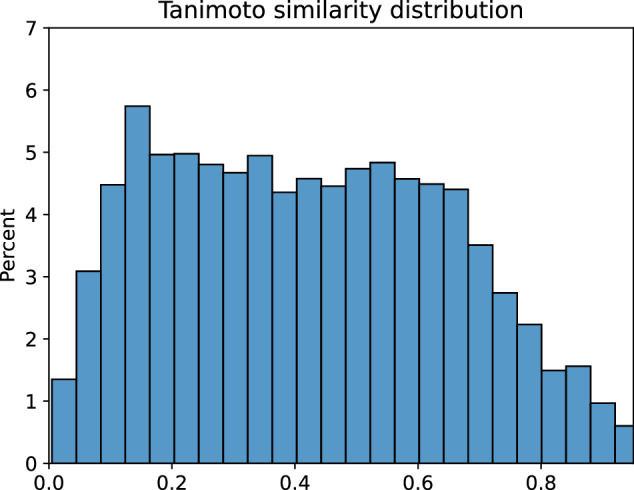
All top--10 predictions of the model to the ground truth. Correct predictions are excluded.

Also speaking to the model’s ability to predict the correct structure is that the interval between 0.0 and 0.2 solely accounts for less than 20% of predictions, and as such the vast majority of predicted molecules are similar to the target molecule. Figure 8 demonstrates this for three randomly chosen molecules with all ten predictions showing high similarity to the target.

Fig. 8. Model prediction examples.

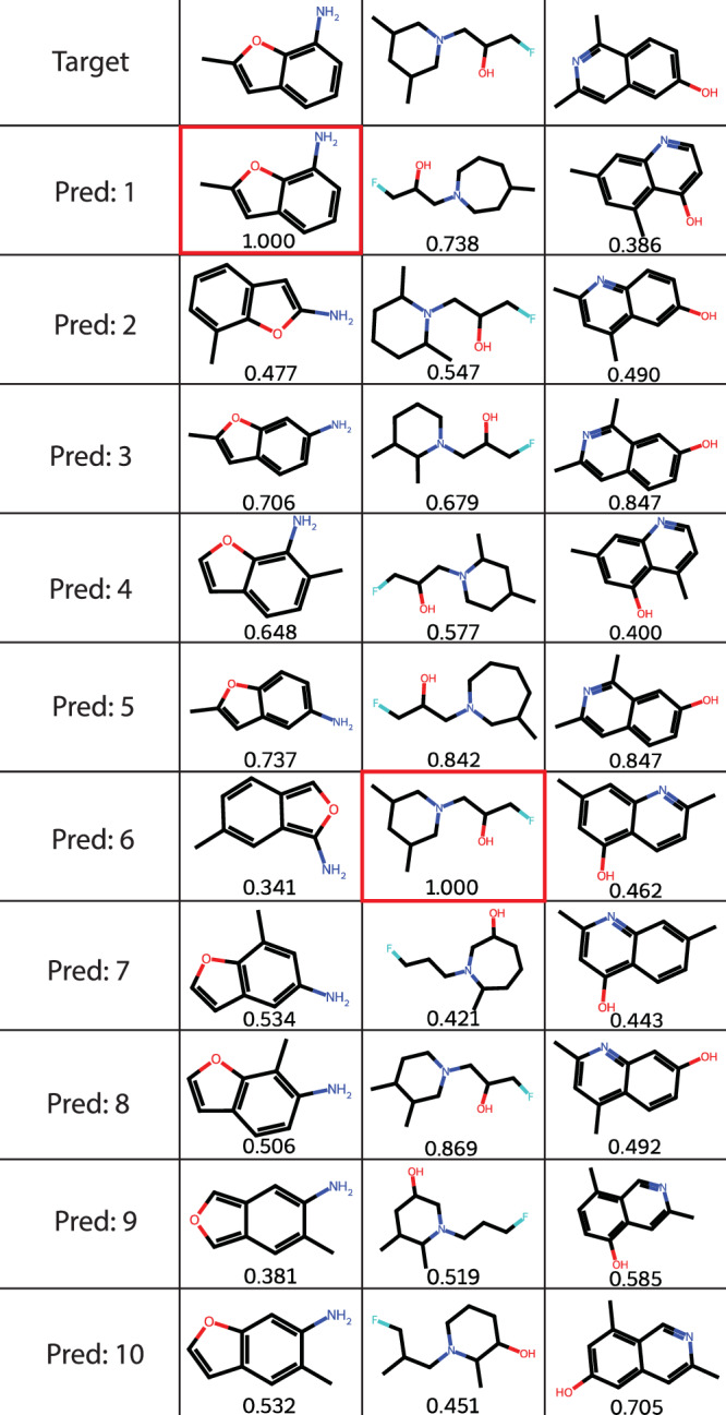
Three different examples of the model predicting a molecule from an IR spectrum. The top row consists of the target, with the predictions in ranked order as predicted by the model below. Correct predictions are highlighted in red and the Tanimoto similarity is given below each predicted structure.

We also assessed the model’s ability to predict the correct scaffold from the IR spectrum. Murcko scaffold’s were constructed using RDKit³⁶. Our model is able to correctly match the scaffold as the top–1 prediction in 84.46%, in the top–5 in 92.27% and in the top–10 in 93.00% of cases.

Limitations

One of the key limitations of our methodological approach lies in the availability of datasets containing infrared spectra. While many such datasets do exist, licences are often expensive and restrict machine learning applications, limiting their use. Consequently, we were compelled to simulate IR spectra using molecular dynamics and force fields for pretraining, before fine-tuning on the relatively small NIST IR dataset. While this approach is not inherently limiting, the NIST dataset only contains 5228 gas-phase IR spectra. Using IR spectra obtained from other instrument types (e.g. Attenuated Reflectance IR, ATR-IR) would likely lead to additional improvements after further fine-tuning. Additionally, while we demonstrated that pretraining on the simulated IR spectra leads to a significant increase in performance, we simulate our spectra using force fields. Leveraging first principle techniques such as DFT could yield further performance increases. However, we chose not to utilise these approaches due to the associated computational cost.

Another limitation is the lack of standardised and openly accessible IR datasets to allow a systematic and rigorous comparison between different models. While we compare our work to that of Fine et al. and Jung et al. the datasets, and as such also the functional group distributions, are different for each of the works.

Conclusions

We have presented a transformer model that for the first time is capable of elucidating the molecular structure directly from experimental IR spectra. Initially, we pretrained our model on simulated IR spectra. Using this baseline model, we fine-tuned and evaluated the model on experimental data. Our best model shows a top–1 performance of 44.39%, top–5 of 66.85% and top–10 performance of 69.79%.

We found that our model is able to correctly predict functional groups with an average F1 score of 0.856, competitive with previous works. Upon analysing the model’s failures in predicting functional groups, we observed that it made errors resembling those a human analyst might commit when interpreting a spectrum. This demonstrates the effectiveness of the model in capturing key features crucial for the interpretation of spectra.

When making errors, the molecules predicted by the model are very similar to the target molecule with an average Tanimoto similarity of 0.487. In addition, when only considering the scaffold our model is capable of predicting the correct scaffold in 84.46% and 93.00% of the top–1 and top–10 predictions, respectively.

By initially training the model on simulated data and subsequently fine-tuning it on experimental data, the model gains the ability to process real-world experimental data while benefiting from the foundational knowledge acquired from simulated data.

With this work, we envision a democratization of structural characterization, a future where the initial structure elucidation of unknown substances can be performed using IR spectroscopy, leaving costly and time-consuming NMR techniques only for final verification or challenging cases. This prospect is particularly advantageous for research institutions that may face limitations in terms of resources and cannot afford complex and expensive analytical instruments.

Methods

Model

We base our model architecture on the Molecular Transformer¹³. The model takes the formatted IR spectrum with the chemical formula as input and outputs a molecular structure encoded as SMILES. This can be formulated as a translation task from the spectrum to the molecular structure. We tokenise SMILES as following Schwaller et. al.¹³. The model is trained to autoregressively predict SMILES, i.e. one token at a time.

The model is implemented using the standard transformer of OpenNMT-py library^37,38 with the following hyperparameters deviating:

word_vec_size: 512

hidden_size: 512

layers: 4

batch_size: 4096

attention_heads: 8

optimiser: adam

adam_beta1: 0.9

adam_beta2: 0.998

decay_method: noam

learning_rate: 2.0

activation_fn: relu

All models are trained for 250k steps amounting to approximately 35h on a V100 GPU. Fine-tuning was carried out for 5000 steps with the same settings as training.

Synthetic data

Using Molecular Dynamics, the spectra of 634,585 molecules were generated. The molecules were sampled from PubChem³⁰ and filtered to exclude charged molecules, stereoisomers, and molecules containing atoms other than C, H, N, O, S, P, and the halogens, while restricting the heavy atom count to a range of 6–13. A molecular dynamics simulation was run for 800,000 molecules sampled from this set.

A high throughput pipeline was developed in Python to orchestrate molecular dynamics simulations and calculate the spectra from the molecule’s dipole moment. The pipeline utilised the Enhanced Monte Carlo (EMC) tool³⁹ to generate the input files for a Large-scale Atomic-Molecular Massively Parallel Simulator (LAMMPS) simulation^40,41. PCFF is utilised as force field²⁶. The system is allowed to equilibrate for 125 ps, before recording the dipole moment of the molecule for a further 125 ps.

IR spectra are calculated from the dipole moment^42,43. Here we use the approach implemented by Braun⁴⁴ using a correlation depth of 10% to ensure statistical sampling.

A total of 634,585 spectra with a resolution of 2 cm⁻¹ and range of 400–3982 cm⁻¹ were successfully generated representing a success rate of 75.6%. Most errors were caused by bond types not being parameterised by PCFF.

Experimental data

Experimental IR spectra were obtained from the National Institute of Standards and Technology (NIST)²⁷. The database contains a total of 5228 gas phase IR spectra. 3108 spectra have a range of 450–3966, while 2120 spectra have a range of 550–3846. Both of the sets as obtained have a resolution of 4cm⁻¹. The experimental spectra were filtered to exclude molecules containing atoms other than C, H, N, O, S, P, and the halogens, while also limiting the heavy atom count to 6–13. After filtering, this yielded 3453 spectra. 721 of the compounds were also contained in the simulated data. These were removed from the set of simulated data yielding a final training set of 633,864 simulated spectra. All further processing steps were carried out identically for experimental and simulated spectra.

Data processing

The input of the model consists of the IR spectrum and the molecular formula. The molecular formula is calculated using RDKit. The input representation of the IR spectrum was obtained by interpolating over the specified range and to a given resolution. All spectra are normalized to the range 0–99 and converted to integers. The molecular formula is split into atom types and numbers and the IR spectrum is appended to this string following the vertical bar, “∣”, as a separating token. All SMILES strings were canonicalised ensuring a consistent molecular representation and tokenized according to Schwaller et al.¹³.

Both the simulated and experimental datasets were split into a training, test and validation set. Test and validation set sizes were set to 10% and 5% for the simulated and 20% and 10% for experimental dataset.

Data augmentation

Both experimental and synthetic data were augmented using the following data augmentation techniques:

• Vertical Noise was added to the spectra by sampling a normal distribution with mean 1 and a standard deviation of 0.05 the maximum value of the spectrum. Mathematically: μ = 1,  σ = 0.05 ⋅ max(spectrum).

• Smoothing was performed using a 1D-Gaussian filter with sigma of 0.75 and 1.25 before interpolating to the desired resolution and window.

• Spectra are Horizontally Shifted by sampling one spectrum starting at 400 cm⁻¹ and one at 402 cm⁻¹.

• Extended Multiplicative Spectral Augmentation (EMSA) is carried out using the code and default settings provided by Blazhko et al.^34,45.

• To augment spectra by an Offset, a constant is sampled from a normal distribution with mean 0.2 of the maximum of the spectrum and standard deviation of 0.05 of the maximum of the spectrum. Mathematically: μ = 0.2 ⋅ max(spectrum),  σ = 0.05 ⋅ max(spectrum)

• Multiplicative augmentation is performed by multiplying the spectrum with a vector of the same length sampled from a normal distribution of with mean of 1 plus the standard deviation of the spectrum and a standard deviation of 0.2. Mathematically: μ = 1 + std(spectrum),  σ = 0.2.

Each augmentation technique yields two augmented spectra. An example for each augmentation is shown in Fig. 9.

Fig. 9. Augmentation Techniques.

The original spectrum is highlighted in blue the augmented in orange.

Author contributions

M.A. and T.L. conceptualised the project. M.A. generated the synthetic data, optimised the machine learning model and analysed the data. A.C.V. supervised the work. The manuscript was written by M.A., T.L. and A.C.V.

Peer review

Peer review information

Communications Chemistry thanks the anonymous reviewers for their contribution to the peer review of this work. Peer reviewer reports are available.

Data availability

The IR spectra generated for this work and on which the models were trained are openly accessible at 10.5281/zenodo.7928396. The raw data for all figures is supplied in Supplementary Data 1.

Code availability

The code for generating the data and training the models is available at https://github.com/rxn4chemistry/rxn-ir-to-structure.

Competing interests

Dr. Teodoro Laino is an Editorial Board Member for Communications Chemistry, but was not involved in the editorial review of, or the decision to publish this article. All other authors declare no competing interests.

Supplementary information

The online version contains supplementary material available at 10.1038/s42004-024-01341-w.

References

- 1.Barnes, R. B. & Bonner, L. G. The early history and the methods of infrared spectroscopy. Am. J. Phys.4, 181–189 (1936). [Google Scholar]
- 2.Coates, J. Interpretation of Infrared Spectra, A Practical Approach. In Ency. Anal. Chem., 10815–10837 (John Wiley & Sons Ltd, 2020).
- 3.Stuart, B. Infrared Spectroscopy. In Analytical Techniques in Forensic Science, 145–160 (John Wiley & Sons, Ltd, 2021). https://onlinelibrary.wiley.com/doi/abs/10.1002/9781119373421.ch7.
- 4.Chen, C.-S., Li, Y. & Brown, C. W. Searching a mid-infrared spectral library of solids and liquids with spectra of mixtures. Vib. Spectrosc.14, 9–17 (1997). [Google Scholar]
- 5.Platte, F. & Heise, H. M. Substance identification based on transmission THz spectra using library search. J. Mol. Struct.1073, 3–9 (2014). [Google Scholar]
- 6.Varmuza, K., Penchev, P. N. & Scsibrany, H. Large and frequently occurring substructures in organic compounds obtained by library search of infrared spectra. Vib. Spectrosc.19, 407–412 (1999). [Google Scholar]
- 7.Gundlach, M., Paulsen, K., Garry, M. & Lowry, S. Yin and yang in chemistry education: the complementary nature of FTIR and NMR spectroscopies. Tech. Rep. (2015).
- 8.Simpson, A. J., Simpson, M. J. & Soong, R. Nuclear magnetic resonance spectroscopy and its key role in environmental research. Environ. Sci. Technol.46, 11488–11496 (2012). [DOI] [PubMed] [Google Scholar]
- 9.Seger, C. Usage and limitations of liquid chromatography-tandem mass spectrometry (LC–MS/MS) in clinical routine laboratories. Wien. Medizinische Wochenschr.162, 499–504 (2012). [DOI] [PubMed] [Google Scholar]
- 10.Dührkop, K., Shen, H., Meusel, M., Rousu, J. & Böcker, S. Searching molecular structure databases with tandem mass spectra using CSI:FingerID. Proc. Natl Acad. Sci.112, 12580–12585 (2015). [DOI] [PMC free article] [PubMed] [Google Scholar]
- 11.Radford, A. et al. Language models are unsupervised multitask learners (2019).
- 12.He, K., Zhang, X., Ren, S. & Sun, J. Deep Residual Learning for Image Recognition http://arxiv.org/abs/1512.03385 (2015).
- 13.Schwaller, P. et al. Molecular transformer: a model for uncertainty-calibrated chemical reaction prediction. ACS Cent. Sci.5, 1572–1583 (2019). [DOI] [PMC free article] [PubMed] [Google Scholar]
- 14.Moret, M. et al. Leveraging molecular structure and bioactivity with chemical language models for de novo drug design. Nat. Commun.14, 114 (2023). [DOI] [PMC free article] [PubMed] [Google Scholar]
- 15.Vaucher, A. C. et al. Inferring experimental procedures from text-based representations of chemical reactions. Nat. Commun.12, 2573 (2021). [DOI] [PMC free article] [PubMed] [Google Scholar]
- 16.McGill, C., Forsuelo, M., Guan, Y. & Green, W. H. Predicting infrared spectra with message passing neural networks. J. Chem. Inf. Model.61, 2594–2609 (2021). [DOI] [PubMed] [Google Scholar]
- 17.Saquer, N., Iqbal, R., Ellis, J. D. & Yoshimatsu, K. Infrared spectra prediction using attention-based graph neural networks. Digit. Discov.3, 602–609 (2024). [Google Scholar]
- 18.Stienstra, C. M. K. et al. Graphormer-IR: Graph Transformers Predict Experimental IR Spectra Using Highly Specialized Attention. J. Chem. Inf. Model.64, 4613–4629. [DOI] [PubMed]
- 19.Enders, A. A., North, N. M., Fensore, C. M., Velez-Alvarez, J. & Allen, H. C. Functional group identification for FTIR spectra using image-based machine learning models. Anal. Chem.93, 9711–9718 (2021). [DOI] [PubMed] [Google Scholar]
- 20.Jung, G., Jung, S. G. & Cole, J. M. Automatic materials characterization from infrared spectra using convolutional neural networks. Chem. Sci.14, 3600–3609 (2023). [DOI] [PMC free article] [PubMed] [Google Scholar]
- 21.Fine, J. A., Rajasekar, A. A., Jethava, K. P. & Chopra, G. Spectral deep learning for prediction and prospective validation of functional groups. Chem. Sci.11, 4618–4630 (2020). [DOI] [PMC free article] [PubMed] [Google Scholar]
- 22.Judge, K., Brown, C. W. & Hamel, L. Sensitivity of infrared spectra to chemical functional groups. Anal. Chem.80, 4186–4192 (2008). [DOI] [PubMed] [Google Scholar]
- 23.Klawun, C. & Wilkins, C. L. Optimization of functional group prediction from infrared spectra using neural networks. J. Chem. Inf. Comput. Sci.36, 69–81 (1996). [Google Scholar]
- 24.Weininger, D. SMILES, a chemical language and information system. 1. Introduction to methodology and encoding rules. J. Chem. Inf. Comput. Sci.28, 31–36 (1988). [Google Scholar]
- 25.Weininger, D., Weininger, A. & Weininger, J. L. SMILES. 2. algorithm for generation of unique SMILES notation. J. Chem. Inf. Comput. Sci.29, 97–101 (1989). [Google Scholar]
- 26.Sun, H., Mumby, S. J., Maple, J. R. & Hagler, A. T. An ab Initio CFF93 All-Atom Force Field for Polycarbonates. J. Am. Chem. Soc.116, 2978–2987 (1994). [Google Scholar]
- 27.NIST Standard Reference Database 35. NIST (2010). https://www.nist.gov/srd/nist-standard-reference-database-35. (Accessed June 5, 2023).
- 28.Bagal, V., Aggarwal, R., Vinod, P. K. & Priyakumar, U. D. MolGPT: molecular generation using a transformer-decoder model. J. Chem. Inf. Model.62, 2064–2076 (2022). [DOI] [PubMed] [Google Scholar]
- 29.Honda, S., Shi, S. & Ueda, H. R. SMILES Transformer: Pre-trained Molecular Fingerprint for Low Data Drug Discovery http://arxiv.org/abs/1911.04738 (2019).
- 30.Kim, S. et al. PubChem 2023 update. Nucleic Acids Res.51, D1373–D1380 (2023). [DOI] [PMC free article] [PubMed] [Google Scholar]
- 31.Beltagy, I., Peters, M. E. & Cohan, A. Longformer: The Long-Document Transformer http://arxiv.org/abs/2004.05150 (2020).
- 32.Krenn, M., Häse, F., Nigam, A., Friederich, P. & Aspuru-Guzik, A. Self-referencing embedded strings (SELFIES): a 100% robust molecular string representation. Mach. Learn.: Sci. Technol.1, 045024 (2020). [Google Scholar]
- 33.O’Boyle, N. & Dalke, A. DeepSMILES: An Adaptation of SMILES for Use in Machine-Learning of Chemical Structures (2018).
- 34.Blazhko, U., Shapaval, V., Kovalev, V. & Kohler, A. Comparison of augmentation and pre-processing for deep learning and chemometric classification of infrared spectra. Chemom. Intell. Lab. Syst.215, 104367 (2021). [Google Scholar]
- 35.Bajusz, D., Rácz, A. & Héberger, K. Why is Tanimoto index an appropriate choice for fingerprint-based similarity calculations? J. Cheminf.7, 20 (2015). [DOI] [PMC free article] [PubMed] [Google Scholar]
- 36.RDKit. https://www.rdkit.org/. (Accessed April 14, 2023).
- 37.OpenNMT-py: Open-Source Neural Machine Translation (2017). https://github.com/OpenNMT/OpenNMT-py. (Accessed April 20, 2023).
- 38.Klein, G., Kim, Y., Deng, Y., Senellart, J. & Rush, A. M. OpenNMT: Open-Source Toolkit for Neural Machine Translation (2017). ArXiv:1701.02810.
- 39.in ’t Veld, P. J. & Rutledge, G. C. Temperature-dependent elasticity of a semicrystalline interphase composed of freely rotating chains. Macromolecules36, 7358–7365 (2003). [Google Scholar]
- 40.Thompson, A. P. et al. LAMMPS - a flexible simulation tool for particle-based materials modeling at the atomic, meso, and continuum scales. Comput. Phys. Commun.271, 108171 (2022). [Google Scholar]
- 41.LAMMPS Molecular Dynamics Simulator. https://www.lammps.org. (Accessed April 20, 2023).
- 42.Thomas, M., Brehm, M., Fligg, R., Vöhringer, P. & Kirchner, B. Computing vibrational spectra from ab initio molecular dynamics. Phys. Chem. Chem. Phys.15, 6608–6622 (2013). [DOI] [PubMed] [Google Scholar]
- 43.Esch, B. V. D., Peters, L. D. M., Sauerland, L. & Ochsenfeld, C. Quantitative comparison of experimental and computed ir-spectra extracted from ab initio molecular dynamics. J. Chem. Theory Comput.17, 985–995 (2021). [DOI] [PubMed] [Google Scholar]
- 44.Braun, E. Calculating An IR Spectra From A Lammps Simulation https://zenodo.org/record/154672. 10.5281/ZENODO.154672 (2016).
- 45.Blazhko, U. Code for Extended Multiplicative Signal Augmentation (2024). https://github.com/BioSpecNorway/EMSA. (Accessed January 28, 2024).
Associated Data
This section collects any data citations, data availability statements, or supplementary materials included in this article.
Supplementary Materials
Description of Additional Supplementary Files
Data Availability Statement