Abstract
Breast cancer (BC) is a type of cancer which progresses and spreads from breast tissues and gradually exceeds the entire body; this kind of cancer originates in both sexes. Prompt recognition of this disorder is most significant in this phase, and it is measured by providing patients with the essential treatment so their efficient lifetime can be protected. Scientists and researchers in numerous studies have initiated techniques to identify tumours in early phases. Still, misperception in classifying skeptical lesions can be due to poor image excellence and dissimilar breast density. BC is a primary health concern, requiring constant initial detection and improvement in analysis. BC analysis has made major progress recently with combining multi-modal image modalities. These studies deliver an overview of the segmentation, classification, or grading of numerous cancer types, including BC, by employing conventional machine learning (ML) models over hand-engineered features. Therefore, this study uses multi-modality medical imaging to propose a Computer Vision with Fusion Joint Transfer Learning for Breast Cancer Diagnosis (CVFBJTL-BCD) technique. The presented CVFBJTL-BCD technique utilizes feature fusion and DL models to effectively detect and identify BC diagnoses. The CVFBJTL-BCD technique primarily employs the Gabor filtering (GF) technique for noise removal. Next, the CVFBJTL-BCD technique uses a fusion-based joint transfer learning (TL) process comprising three models, namely DenseNet201, InceptionV3, and MobileNetV2. The stacked autoencoders (SAE) model is implemented to classify BC diagnosis. Finally, the horse herd optimization algorithm (HHOA) model is utilized to select parameters involved in the SAE method optimally. To demonstrate the improved results of the CVFBJTL-BCD methodology, a comprehensive series of experimentations are performed on two benchmark datasets. The comparative analysis of the CVFBJTL-BCD technique portrayed a superior accuracy value of 98.18% and 99.15% over existing methods under Histopathological and Ultrasound datasets.
Keywords: Transfer learning, Breast cancer, Computer vision, Horse Herd Optimization Algorithm, Image preprocessing
Subject terms: Computer science, Information technology
Introduction
The WHO described that cancer is the crucial reason for non-accidental deaths globally; around 8.8 million people died from cancer in 20151. BC is a fatal and common syndrome among women globally. Hence, initial and accurate diagnosis plays an essential part in increasing the prediction and enhancing the patient’s survival rate with breast tumours from 30 to 50%. Generally, BC has two categories: malignant and benign. Malignant is cancerous (invasive), whereas Benign is a noncancerous (non-invasive) cancer type2. Both tumours have additional subcategories that want to be diagnosed individually because each might lead to various prediction and treatment strategies. Medical imaging conditions are generally more effective and adopted for BC recognition than other testing techniques. Standard medical imaging conditions for BC analysis are ultrasound imaging, magnetic resonance imaging (MRI), mammography, computed tomography (CT), and histopathology images3. Histopathology is the procedure of total estimation and microscopic review of biopsy tissue specimens performed by a diagnostician or specialist to learn about cancer growing in organs or tissues4. Regular histopathologic samples have other cells and structures surrounded and dispersed haphazardly by different tissue types. The manual examination of historical images and the vision inspection take time. The utilities of computer-based image investigation denote an efficient model to increase histopathology images’ analytical and predictive skills5. Moreover, Ultrasound imaging can be helpful in the prognosis and identification of BC because of its real-time imaging, non-invasive, high image resolution, and non-radioactive. Nevertheless, the analysis of ultrasound images requires highly trained and proficient radiologists. Generally, the computer-aided diagnosis (CAD) method has been used in all imaging conditions and analysis types. CAD would be beneficial for radiologists in the classification and detection of BC6.
They have been improved to reduce expenses and enhance the radiologist’s capacity for medical imaging analysis. The beginning of digital images in the medical field has given an edge to artificial intelligence (AI) for pattern recognition using a CAD process. CAD methods are intended to help doctors by automatically analyzing images. Therefore, such systems lessen human dependence, improve the diagnosis rate, and ease the complete treatment expenditures7. ML is abundantly required in object recognition, text classification, and image recognition. With the development of CAD technologies, ML has been efficiently applied to diagnose BC. Classification of histopathologic images connected to traditional ML methods and simulated extraction of features requires a physical features model; still, it doesn’t require a tool through more efficacy, and it has advantages in computing time8. Still, the classification of histopathologic images associated with deep learning (DL), mainly convolutional neural networks (CNN), often requests more labelled training methods. It aids in classifying and detecting BC in an initial phase. The requirement for improved BC diagnosis stems from its high incidence and crucial impact on women’s health worldwide. Early and precise detection of breast tumours is significant for enhancing treatment outcomes and survival rates9. Conventional diagnostic models often need to improve distinguishing between diverse tumours, accentuating the need for advanced methods. Leveraging computer vision (CV) and multi-modality medical images presents an innovative model to address these threats. Incorporating diverse imaging modalities can provide a more comprehensive understanding of tumour characteristics. This multifaceted strategy improves diagnostic accuracy and eases personalized treatment plans, ultimately aiming to enhance patient prognosis10.
This study uses multi-modality medical imaging to propose a Computer Vision with Fusion Joint Transfer Learning for Breast Cancer Diagnosis (CVFBJTL-BCD) technique. The presented CVFBJTL-BCD technique utilizes feature fusion and DL models to effectively detect and identify BC diagnoses. The CVFBJTL-BCD technique primarily employs the Gabor filtering (GF) technique for noise removal. Next, the CVFBJTL-BCD technique uses a fusion-based joint transfer learning (TL) process comprising three models, namely DenseNet201, InceptionV3, and MobileNetV2. The stacked autoencoders (SAE) model is implemented to classify BC diagnosis. Finally, the horse herd optimization algorithm (HHOA) model is utilized to select parameters involved in the SAE method optimally. To demonstrate the improved results of the CVFBJTL-BCD methodology, a wide series of experimentations are performed on two benchmark datasets. The key contribution of the CVFBJTL-BCD methodology is listed below.
The CVFBJTL-BCD model utilizes the GF approach for efficient noise reduction during the data preprocessing. This method also improves the quality of the input data, resulting in enhanced performance in subsequent analysis. Addressing noise effectively confirms more reliable results in BC classification.
The CVFBJTL-BCD methodology utilizes a joint TL model that integrates three advanced models, namely DenseNet201, InceptionV3, and MobileNetV2. This incorporation also implements the merits of every technique to improve feature extraction and classification accuracy. As a result, it substantially enhances the overall efficiency of BC diagnosis.
The CVFBJTL-BCD model employs the SAE technique to classify BC diagnoses precisely. This methodology effectually learns intrinsic patterns in the data, enabling greater accuracy in distinguishing between diverse cancer types. Optimizing the classification process contributes to more reliable diagnostic outcomes.
The CVFBJTL-BCD technique optimizes the HHOA model to choose parameters for the SAE method. This optimization improves the approach’s performance by fine-tuning crucial parameters and improving classification output. Effectively enhancing parameter selection confirms more precise and reliable BC diagnoses.
The CVFBJTL-BCD method incorporates advanced noise removal, diverse TL models, and innovative optimization methods into a cohesive framework for enhanced BC classification. This overall methodology improves the model’s data quality and performance and allows for greater adaptability across varying datasets. The novelty is its seamless integration of these elements, substantially enhancing diagnostic accuracy and reliability in clinical settings.
The article is structured as follows: Section "2" presents the literature review, Sect. "3" outlines the proposed method, Sect. "4" details the results evaluation, and Sect. "5" concludes the study.
Related works
Sushanki et al11. present an overview of the recent techniques and developments in multi-modal imaging for BC detection. While radiomics, a quantifiable research of imaging data, has been combined using ML and DL methods, breast lesions are displayed as much as possible. These methods could assist in differentiating between malignant and benign tumours, offering doctors critical information. During the several stages of BC recognition, novel techniques are advanced for improvement, classification, segmentation, and feature extraction, utilizing numerous image modalities. Abdullakutty et al12. examined the developing area of multi-modal methods, especially combining HI with non-image data. This article uses multi-modal data and highlights explainability to improve the precision of diagnosis, patient engagement, and clinician confidence, eventually raising more customized treatment tactics for BC. Oyelade et al13. propose a new DL method incorporating TwinCNN methods for addressing the challenges of BC image identification from multi-modalities. Initially, modality-based feature learning was attained by extracting either high- or low-level features utilizing the networks embedded by TwinCNN. In addition, to tackle the infamous issue of highly dimensional features related to the extracted features, the binary optimizer technique has been improved to remove nondiscriminant features efficiently in the search space. Hu et al14. present new methods for the survival prediction of BC, called GMBS. GMBS initially describes a sequence of multi-modal fusing components to incorporate various modalities of patient data, compromising robust early embeddings. Afterwards, GMBS proposes a patient-patient graph creation component, intending to describe the relationship of interpatients efficiently. Finally, GMBS combines a GCN method to utilize the complex architectural data encrypted in the created graph.
Yang et al15. present a new multiple-attention interaction network for BC identification based on the images of DWI and ADC. A three-intermodality interaction mechanism has been demonstrated to ultimately unite the multi-modality data. Three model connections are performed over the advanced intermodality relative component, multilevel attention fusion component, and channel interaction module to study discriminative, correlation, and complementary information. Guo et al16. present a multi-modal BC diagnosis technique based on Knowledge Augmented DL called KAMnet. This technique combines the 3 forms of previous knowledge into DNN over various incorporation tactics. Initially, a temporal segment-selecting approach led by Gaussian sampling over data level incorporation was developed to direct the method to concentrate on keyframes. Next, the author creates a feature fusion network for structure-level incorporation and attains collective interpretation by decision-level incorporation, enabling the exchange of multi-modal data. Zhang et al17. present the MoSID method that extracts inter or intra-modality attention maps as previous knowledge to conduct cancer segmentation from multi-parametric MRI. This can be attained by separating modality-specific data, which offers corresponding signs to the segmentation task and creating modality-specific attention mapping in a creation method. Yan et al18. present the TDF-Net for identifying BC utilizing partial multi-modal ultrasound data. Firstly, this technique proposes a double branch feature extraction component to seizure modality-specific information. Karthik et al19. introduce a tumour lesion segmentation methodology using advanced CNNs on combined MRI and PET scans. It also employs four pre-trained models, namely VGG 19, ResNet 50, SqueezeNet, and DenseNet 121—fine-tuned on ISL datasets, and utilizes a weighted voting ensemble for improved prediction accuracy.
Atrey, Singh, and Bodhey20propose a hybrid framework that integrates a residual neural network (ResNet) with ML for classifying BC images from mammography and ultrasound. Features are extracted, fused, and classified as benign or malignant using a support vector machine (SVM). Subaar et al21. utilize TL from a Residual Network 18 (ResNet18) and Residual Network 34 (ResNet34) architectures to detect BC. Chi et al22. introduce a dual-branch network with a cross-modality attention mechanism for thyroid nodule diagnosis, incorporating CEUS videos and ultrasound images. It employs two transformers—UAC-T for segmenting CEUS features and CAU-T for guiding classification—optimized through multi-task learning. Li et al23. present nn-TransEC, a 3D TL framework based on nnU-Net that integrates segmentation and classification for endometrial cancer T-stage classification. It features nn-MTNet for multi-task learning and a knowledge-embedded ROI tokenization method (KRT) replicating doctors’ workflows by cropping key regions from CT volumes based on prior segmentation. Rahman, Khan, and Babu24introduce the “BreastMultiNet” framework by utilizing the TL model to detect diverse BC types using two public datasets. Hasan et al25. present a computer-assisted methodology for classifying ultrasound lung images using a fuzzy pooling-based CNN (FP-CNN) model. The Shapley Additive Explanation (SHAP) method is employed to clarify the FP-CNN predictions of the model and illustrate the decision-making process. Hossain et al26. introduce a fast, automatic COVID-19 detection technique using chest CT scans. After preprocessing, the model also fuses features from VGG-19 and ResNet-50, identifies key features with Principal Component Analysis (PCA), and classifies them using Max Voting Ensemble Classification (MVEC) methods.
Hasan et al27. developed a model integrating hand-crafted and automated feature extraction. The study also utilized multi-criteria frame selection. Hossain et al28. present a variational quantum circuit (VQC)-based technique using an optimized feature set. Features are optimized with minimum redundancy, maximum relevance (mRMR), and PCA methods. Furthermore, a rule-based expert system is presented. Mostafiz et al29. integrate curvelet transform and CNN features extracted from the preprocessed MRI sequence of the brain. Relevant features are chosen from the feature vector using mutual data based on the minimum redundancy maximum relevance (mRMR) methodology. The detection is done by employing the ensemble classifier of the bagging method. Ai et al30. propose the Self-and-Mutual Attention (SAMA) model. This technique features a module with three stages: improving modality-specific features, bidirectional cross-guidance for refinement, and optimized feature aggregation for precise predictions. Nakach, Zerouaoui, and Idri31employs multi-scale ensembles. Three pre-trained models, DenseNet 201, MobileNet v2, and Inception v3, are utilized across four magnification factors. Predictions are fused with weighted voting and seven meta-classifiers, with top models selected by using the Scott–Knott test and ranked by Borda count voting. Mukhlif, Al-Khateeb, and Mohammed32utilize advanced TL models. The modified Xception model is used to classify histological images. Mukhlif, Al-Khateeb, and Mohammed33present Dual TL (DTL), utilizing pattern convergence between source and target domains. It utilizes this method for VGG16, Xception, ResNet50, and MobileNetV2, fine-tuning unclassified and limited classified images and using data augmentation for enhanced sample size and class balance. Ali and Mohammed34 aim to review and analyze the efficiency of AI methods in omics data analysis.
The existing studies exhibit limitations in methodologies for BC detection. A reliance on imaging data may restrict applicability when datasets are insufficient, while multi-modal methods can complicate integration and reduce effectiveness. Methodologies like TwinCNN may need help with high-dimensional data, resulting in overfitting. Some models need massive datasets for effectual training, and intrinsic interaction mechanisms can increase computational demands. Concerns also arise regarding the robustness of models that rely on prior knowledge integration, as segmentation methods may falter with diverse cancer types. Moreover, performance can vary based on the choice of pre-trained models, and reliance on predefined ROI tokenization might hinder feature capture. Variability in ultrasound imaging conditions additionally complicates classification. These threats underscore the requirement for more adaptable and efficient diagnostic frameworks in clinical settings. Despite enhancements in BC detection models, crucial research gaps remain, specifically in addressing the incorporation of multi-modal data and optimizing model robustness across diverse datasets. Many existing models need help with high-dimensional data and overfitting, while the reliance on predefined features often limits their adaptability. Furthermore, the variability in imaging conditions and the requirement for massive datasets hinder the development of universally applicable outcomes. Thus, there is a significant requirement for more efficient, flexible, and interpretable frameworks in clinical practice.
Proposed methodology
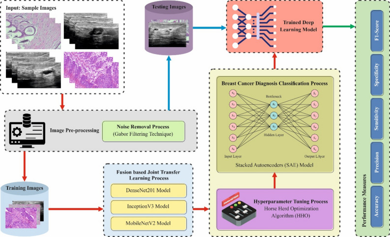
This research proposes a novel CVFBJTL-BCD technique using multi-modality medical imaging. The presented CVFBJTL-BCD technique uses feature fusion and DL models to effectively detect and identify BC diagnosis. It comprises four stages: image preprocessing, feature fusion, classification, and parameter tuning. Figure 1 illustrates the entire flow of the CVFBJTL-BCD approach.
Fig. 1.
Overall flow of CVFBJTL-BCD approach.
Noise reduction
The presented CVFBJTL-BCD technique primarily applies GF for noise removal35. This model is chosen for its effectiveness in conserving significant spatial frequency data while reducing unwanted noise. GFs are appropriate for image processing tasks, specifically medical imaging because they can efficiently detect textures and patterns at diverse scales and orientations. This adaptability allows for an enhanced feature extraction, which is significant for precise diagnosis. Compared to other noise removal approaches, such as Gaussian filtering, the GF model provides superior edge preservation, confirming that critical features are not blurred. Moreover, its mathematical foundation enables precise control over the filter parameters, making it versatile for diverse imaging modalities. Overall, utilizing GF improves the quality of the input data, resulting in enhanced outcomes in subsequent analysis and classification tasks. Figure 2 illustrates the structure of the GF model.
Fig. 2.
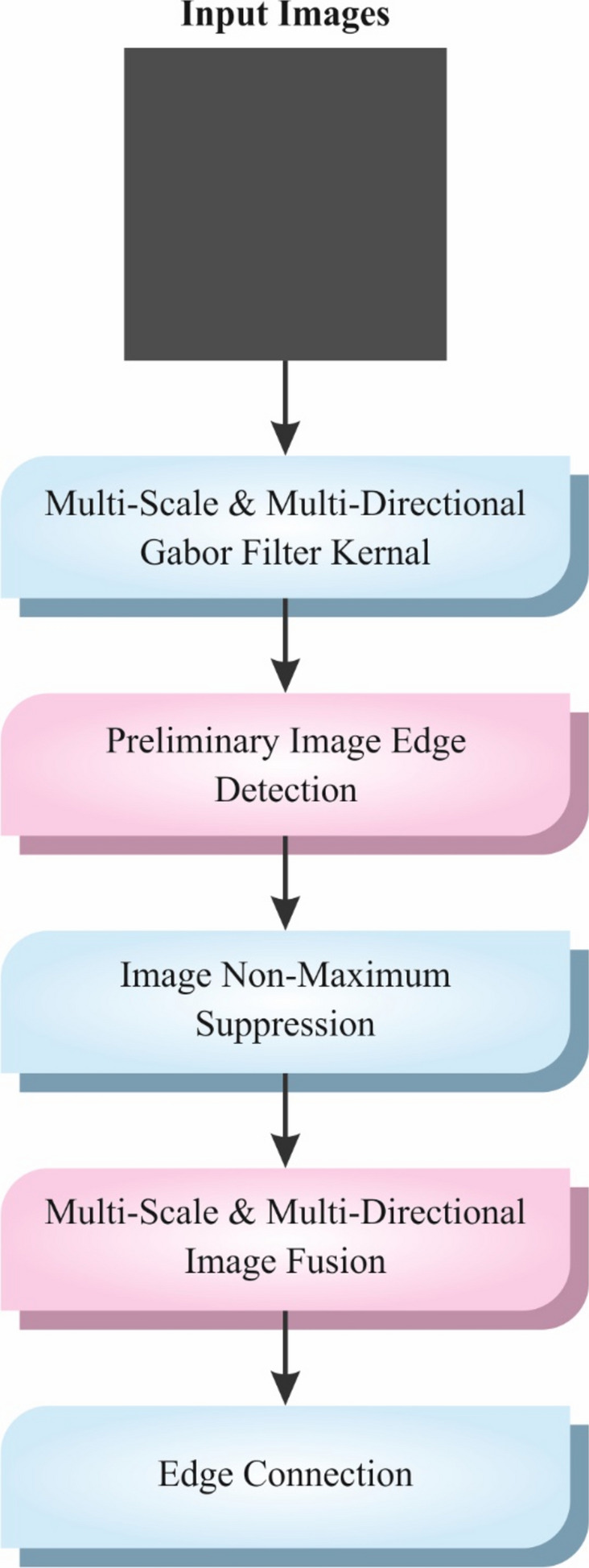
Workflow of GF technique.
The texture is crucial for differentiating the ROIs of dissimilar image classes. Texture study is essential for the analysis of computerized distribution. In ROIs, cancers contain micro patterns in numerous directions and frequencies. These forms are significant in classifying critical areas in a CAD method. GFs are effectively employed to recognize these patterns. GFs are linear filters used in numerous works in CV issues like face identification, texture analysis, and cancer diagnosis. An inspiring feature of GFs is that they have the finest united localization in spatial and frequency fields. To get the mammogram value, GFs of distinguished routes are employed to transfer mammograms by defining the finest extent of GF parameters, and the standardized mammogram is an output. These filters are denoted in mathematical formulations as given below:
| 1 |
whereas denotes filter orientation, means the ratio of spatial feature, represents sinusoidal wavelength, refers to standard deviation, and ø refers to the off-set of phase.
Feature fusion process
Next, the CVFBJTL-BCD method utilizes a fusion-based joint TL process comprising three models, namely DenseNet201, InceptionV3, and MobileNetV2. These models are chosen due to their merits in complementary feature extraction and classification. The DenseNet201 model outperforms at capturing complex patterns through its dense connectivity, which fosters better gradient flow and feature reuse. Also, the InceptionV3 method presets a multi-scale approach, effectually detecting features at diverse resolutions, making it robust against discrepancies in input data. MobileNetV2 is designed for effectiveness, giving high accuracy with mitigated computational costs, making it ideal for resource-constrained environments. By incorporating these models, the methodology employs diverse architectures to improve performance, increase generalization across diverse datasets, and improve overall predictive accuracy in complex classification tasks. This ensemble method also reduces the weaknesses of individual models, resulting in a more robust and efficient outcome.
While global features cover comprehensive data, the present redundancy frequently declines attention to the primary information36. To evade this concern, some approaches trust local features to remove terminated data intrusion by segmentation but might disregard the link. Removing local and global features analogously and openly combining them is a usual feature extraction tactic. On the other hand, this approach generally trades the significance of local and global feature extraction. To improve the correlation amongst dissimilar features, an effective technique uses a weighted sharing fully connected (FC) layer in a multi-task joint learning system. In the meantime, a multi‐loss device is designed to assist network training in stabilizing the significance of local and global features. For local features, the segmentation can remove the terminated data in the feature for improvement. So, the joint learning network employs a patch layer for segmenting an input image (signified as I ) into numerous patch‐level imageries through the form of and loads them as per the size of the channel. The attained patch‐level tensor is denoted as:
| 2 |
Meanwhile, signifies the patch‐level image.
Next, a technique is used to pick the convolution (Conv) layer with the kernel dimension in the local branch to remove local features. The task is used to familiarize non-linearity. The function presents few trainable parameters and has improved the drive of network weights and increased detection accuracy.
To decrease the intricacy, the global average pooling layer is utilized to compact the local branch output (signified as ) and acquire the compacted feature :
| 3 |
Here, indicates the global average pooling layer. Next, the local feature is mined as:
| 4 |
Here, specifies the FC layer.
Likewise, by following the FC and global average pooling layers, the global feature is attained as:
| 5 |
where
| 6 |
denotes the FC layer, and signifies the global average pooling layer.
A straight mixture of local and global features can cover both. The method restrains the training of multi‐task joint learning networks depending upon the backward loss of straight fusion feature to ensure that the critical local and global feature data were well-kept after the synthesis. and are attained by compression through the global average pooling layer to achieve local and global features. When equated with and , and are not managed by FC layer training weights, so they could more efficiently mine local and global data. Now, and are combined directly with a similar ratio as :
| 7 |
Meanwhile, denotes the concatenate operation.
DenseNet201
The design of the DenseNet201 structure uses densely connected blocks, permitting every layer to obtain straight input from each prior layer37. This helps feature reprocess and recover the flow of gradient. The structure includes numerous dense blocks, each containing densely associated convolutional layers. Transition layers were employed to allow downsampling over pooling and dimensional reduction. Non‐linearity and constant training are endorsed by using and BN after every convolutional layer. The network is determined with global mean pooling that is tracked by a completely connected layer, and the activation function of is utilized for multiclass classification. Figure 3 illustrates the structure of DenseNet201.
Fig. 3.
Framework of DenseNet201.
InceptionV3
InceptionV3 is an exact neural network structure aimed at constantly detecting images. The network uses many inception components integrating parallel convolutional processes of diverse kernel dimensions, assisting the effectual capturing of features at numerous spatial measures. The inception component includes convolutional layers with pooling operations and numerous filter sizes, permitting the method to remove a vast range of distinct features from input imageries. Furthermore, InceptionV3 integrates support classifiers to tackle the problem of vanishing gradient in training. Furthermore, it uses BN and factorized 7 × 7 convolution (Conv) to reduce computational complexity while attaining higher performance. The structure is highly considered for its ability to operate numerous visual detection tasks with exceptional precision effectively. Figure 4 signifies the architecture of the InceptionV3 model.
Fig. 4.
Architecture of InceptionNetV3 model.
MobileNetV2
MobileNetV2 is a very effectual CNN design that uses linear constraints and depth‐wise segmented Conv to equalize computation complexity and accuracy. The structure includes numerous reversed residual blocks; every one contains convolutional layers, , and BN. Additionally, MobileNetV2 employs shortcut connections and development to increase the flow of data and feature reprocessing among layers. MobileNetV2 is appropriate for present object detection and image identification tasks on gadgets with restricted sources, lightweight operations, and effectual design ethics. Figure 5 demonstrates the architecture of the MobileNetV2 technique.
Fig. 5.
Structure of MobileNetV2 model.
Classification using the SAE model
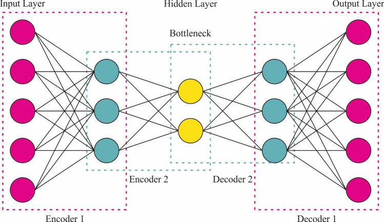
For the classification of BC diagnosis, the SAE model is exploited. The SAE network is an extensively applied DL architecture that contains two key modules of stack encoders (recognizing network) and decoders (generating network)38. This technique is selected for classification due to its capability to learn hierarchical representations of data, which is specifically beneficial for intrinsic datasets. The model captures increasingly abstract features by stacking various layers of autoencoders, allowing for enhanced feature extraction and dimensionality reduction. This capability improves the model’s performance in tasks where conventional methodologies might face difficulty detecting relevant patterns. Furthermore, SAEs are robust to noise and can efficiently handle high-dimensional data, making them appropriate for medical imaging applications. Compared to other classification methods, namely SVMs or decision trees (DTs), SAEs can utilize unsupervised learning to pre-train on unlabeled data, which can be advantageous in scenarios with limited labelled examples. This results in an improved generalization and improved accuracy in classification tasks. Figure 6 shows the architecture of the SAE methodology.
Fig. 6.
SAE framework.
It portrays a proportioned structure with equivalent hidden neuron counts in the encoder and decoder layers. The encoding layers intellectualize the new input signals (now, multiple‐element data concentration) into deeply featured codings that measure numerous top-level illustrations of multivariant signals (where high-level representations of geochemical background populations). These decoding layers utilize but are deeply featured codings for generating the output signals such that they are equivalent to the input signal’s structure. The encoding and decoding non-linear functions for an experimental feature vector are described as
| 8 |
| 9 |
whereas and represent functions of encoding and decoding in hidden layer (HL) () and HL , correspondingly. The and signify weighted matrices in and , whereas and showed biased vectors in and , individually. The formulations ( and symbolize activation functions of and appropriately, and they might be adjusted through tasks like a hyperbolical tangent, linear, Maxout unit, sigmoid, step, , and ReLU. Throughout fine‐tuning in BP, the error results are utilized to upgrade the network‐wide parameter over gradient background techniques to attain an experienced network of SAE.
HHOA-based parameter tuning
Eventually, the HHOA approach is applied to optimally select parameters involved in the SAE method. The HHOA model is employed for optimal parameter selection in the SAE method due to its effectualness in exploring intrinsic search spaces and finding optimal solutions. The HHOA methodology is inspired by horses’ natural behaviour, allowing it to balance exploration and exploitation effectually, which is significant for parameter tuning in DL methods. Compared to conventional optimization approaches such as grid or random search, HHOA is faster and often more efficient in converging to optimal or near-optimal solutions. Its population-based approach enables it to avert local minima, improving the likelihood of attaining enhanced overall performance. Furthermore, the adaptability of the HHOA model makes it appropriate for dynamic environments, allowing for fine-tuning in real-time as new data becomes available. This results in an enhanced accuracy and robustness of the SAE model in classification tasks. Figure 7 depicts the overall structure of the HHOA model.
Fig. 7.
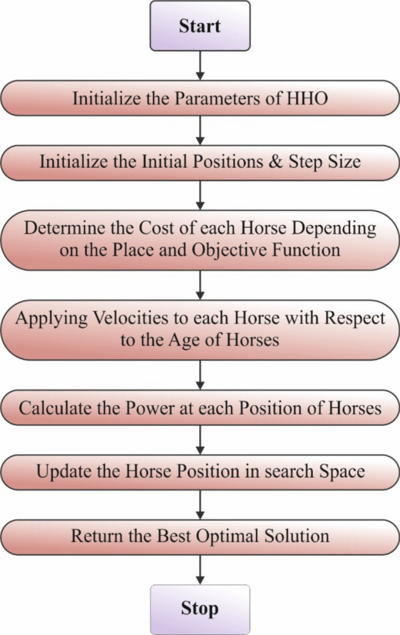
Structure of HHOA model.
The HHOA approach was advanced depending on the horses behaviour in their natural world at different ages39. Generally, the behaviour of horses is split into six types: Hierarchy, Grazing, Defense Mechanism, Sociability, Roaming, and Imitation. Each horse transfers based on the subsequent Eq. in every iteration:
| 10 |
Here, establishes horse location, offerings horse velocity, specifies the age limit of every horse, and displays the present iteration. Every horse’s velocity has been computed depending on its age range and its behavioural patterns inside an iteration.
| 11 |
After this, individual and social intellect work for horses is considered.
Grazing (G)
Grazing is a normal horse behavioural pattern. Horses pasture approximately 70% on time in the day and 50% at night. People of all ages use roughly 16 to 20 h of daily pasture on pastures. The pasture area of every horse can be displayed using the HHOA method using the coefficient Eqs. (12) and (13) define graze mathematics.
| 12 |
| 13 |
Now, calculates the trend of the horse to grazing, which reduces linearly by at every iteration. Furthermore, and specify the lower and upper boundaries of the pasture field correspondingly, whereas represents a random number among and .
Hierarchy (H)
It is possible to find a hierarchy amongst horses every time since there are farm animals. The hierarchy safeguards horses but also permits them admittance to improved feeding lands. In the HHOA model, the coefficient characterizes the horse’s trend to track the horse with the best strength and knowledge. Various studies have presented that within the Middle Ages, and , horses will have a behavioural hierarchy. Equations (14) and (15) define hierarchical behaviours as given below:
| 14 |
| 15 |
Here establishes the best location for horses, and illustrates how the best location affects the velocity parameter.
Sociability (S)
Social behaviour is a horse’s characteristic. Sociability intends to improve predator-protecting methods and reduce scanning time. Additionally, sociability raises intra‐group conflicts and competition, transmission of diseases, and the threat of attracted predators. Since flight represents the best-protected method for horses, it is fundamental to detect unseen predators immediately. Hence, the capacity for maintaining group awareness, acting as a cluster in the flight, and communicating efficiently about these activities will be of major significance for every horse of a flock. Factor determines the horse’s social behaviour, which can be designated in the subsequent Eqs. (16) and (17).
| 16 |
| 17 |
represents the social movement vector horse , which reduces per iteration in the factor. Moreover, denotes total horse counts. AGE states the age range of horses. Still, the average location has been gained in the following:
| 18 |
Imitation (I)
As social animals, horses will learn from one another about fine and bad behaviour, like finding appropriate ground. Younger horses tend to mimic new horses during the age limit of 0‐5 years. Additionally, factor in the HHOA method shows this characteristic of the behaviour of horses. Simulated in horse herds is described below:
| 19 |
| 20 |
determines horse movement near the mean location of the finest horses positioned at specifies horse counts within the finest area. The mentioned p-value is 10% of the total horses. Besides, is stated as a reducing factor for every iteration, as revealed earlier. Also, the finest position can be gained in the succeeding Eq. (21).
| 21 |
Defense mechanism (D)
Horses have dual main protection methods: fight and flight. Once challenged with a critical condition, horses typically flee, and fighting helps as a subordinate protective method. Factor defines the survival procedure of horses. Equations (22) and (23) with negative coefficients signify the survival mechanisms of horses, which stop them from reaching unsuitable locations.
| 22 |
| 23 |
symbolizes the fleeing vector of the horse , depending on the horse’s mean in the poor parts. The horse counts with the poorest positions are also exposed to . equates to 20% of each horse. As previously specified, characterizes the reducing factor for every iteration. Still, the poorest location has been considered in the following:
| 24 |
Roaming (R)
By the age limit of 5 to 15 years, young horses also tended to transfer from grazing to pasture in search of nutrition. Horses were interested animals who searched for novel grazing where they could. As horses attain adulthood, they reduce their behaviour by roaming. The factor displays this horse’s behaviour for randomized motion in Eqs. (25) and (26).
| 25 |
| 26 |
In such a case, horse’s randomly generated velocity vector, and its reducing factor is designated by . To compute the total velocity, the sociability, grazing, defence method, imitation, hierarchy, and roaming were replaced in Eq. (11).
By using a sorting method across a global matrix, HHOA utilizes a suitable methodology to boost the speediness of problem resolution whereas moreover evading local optimum entrapment. Equations (27) and (28) represent the global matrix that can be made by juxtaposing locations (X) and the value of cost for each location .
| 27 |
| 28 |
The HHOA method develops a fitness function (FF) to improve classification performance. It identifies a positive integer to signify the enhanced performance of the candidate solutions. In this research, the minimization of the classification rate of error can be identified as an FF, as specified in Eq. (29).
| 29 |
Experimental validation
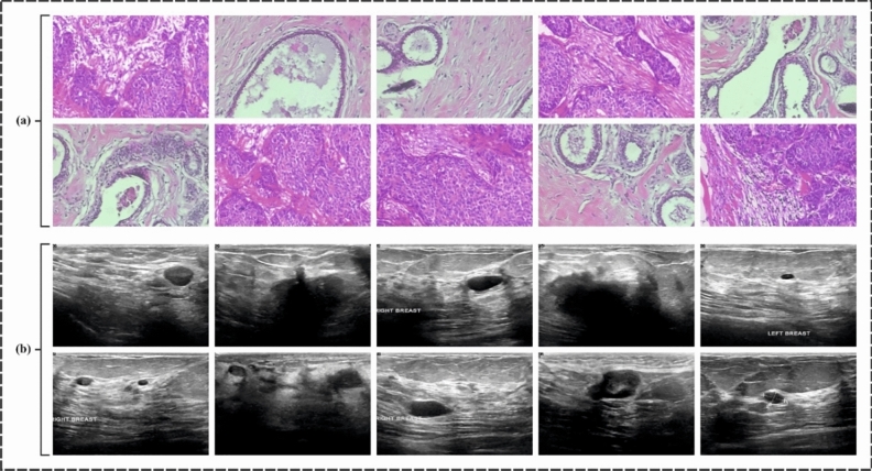
In this sector, the CVFBJTL-BCD model’s experimental validation is verified using the histopathological datasets40and the Ultrasound dataset41. The histopathological dataset comprises 9,109 microscopic images of breast tumour tissue from 82 patients, categorized into 2,480 benign and 5,429 malignant samples. The images are collected utilizing the SOB approach (excisional biopsy) at diverse magnifications (40X, 100X, 200X, and 400X) in PNG format, measuring 700 × 460 pixels with 8-bit RGB depth. The ultrasound dataset, accumulated over a year at Baheya Hospital in DICOM format, initially encompasses 1,100 grayscale images but was refined to 780 after preprocessing to remove duplicates and irrelevant data. Scans were performed by employing LOGIQ E9 ultrasound systems, giving 1280 × 1024 pixel resolution images. Preprocessing encompasses annotation corrections and conversion to PNG, with ground truth boundaries established using MATLAB through freehand segmentation. The datasets are organized into folders by cancer type, with filenames indicating class and including a “_mask” suffix for segmented images. Figure 8 denotes the sample images of two datasets. The histopathological 200X dataset contains 2013 images under 2 classes as shown in Table 1. The suggested technique is simulated using the Python 3.6.5 tool on PC i5-8600 k, 250 GB SSD, GeForce 1050Ti 4 GB, 16 GB RAM, and 1 TB HDD. The parameter settings are provided: learning rate: 0.01, activation: ReLU, epoch count: 50, dropout: 0.5, and batch size: 5.
Fig. 8.
Sample Images (a) Histopathological Images (b) Ultrasound Images.
Table 1.
Details on Histopathological Dataset.
| Histopathological dataset 200X | |
|---|---|
| Class | No. of images |
| Benign | 623 |
| Malignant | 1390 |
| Total images | 2013 |
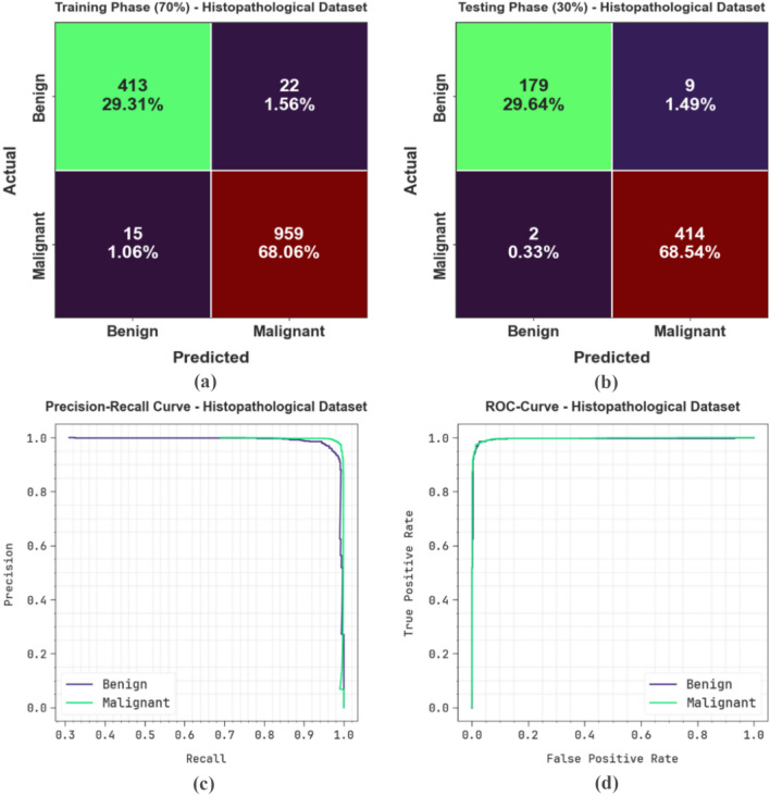
Figure 9 represents the classification outcomes of the CVFBJTL-BCD process on the Histopathological dataset. Figure 9a-9b displays the confusion matrix with precise identification and classification of all class labels on a 70:30 TRAP/TESP. Figure 9c demonstrates the PR analysis, indicating maximum performance across all classes. Lastly, Fig. 9d represents the ROC analysis, showing efficient results with high ROC values for distinct class labels.
Fig. 9.
Histopathological dataset (a-b) Confusion matrices and (c-d) PR and ROC curves.
In Table 2 and Fig. 10, the BC detection outcomes of the CVFBJTL-BCD model are represented on the Histopathological dataset. The results reported that the CVFBJTL-BCD process discriminated adequately between benign and malignant samples. On 70%TRAP, the CVFBJTL-BCD technique offers an average of 97.37%, of 97.13%, of 96.70%, 96.70% and of 96.91%. Moreover, on 30%TESP, the CVFBJTL-BCD approach provides an average of 98.18%, of 98.38%, of 97.37%, 97.37%, and of 97.85%.
Table 2.
BC detection outcomes of CVFBJTL-BCD technique on Histopathological dataset.
| Class | |||||
|---|---|---|---|---|---|
| TRAP (70%) | |||||
| Benign | 97.37 | 96.50 | 94.94 | 98.46 | 95.71 |
| Malignant | 97.37 | 97.76 | 98.46 | 94.94 | 98.11 |
| Average | 97.37 | 97.13 | 96.70 | 96.70 | 96.91 |
| TESP (30%) | |||||
| Benign | 98.18 | 98.90 | 95.21 | 99.52 | 97.02 |
| Malignant | 98.18 | 97.87 | 99.52 | 95.21 | 98.69 |
| Average | 98.18 | 98.38 | 97.37 | 97.37 | 97.85 |
Fig. 10.
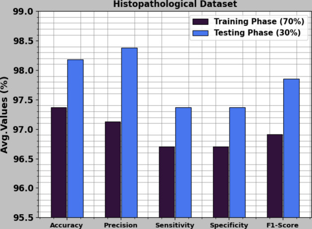
Average of CVFBJTL-BCD technique on Histopathological dataset.
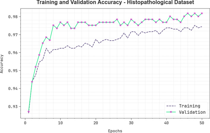
Figure 11 illustrates the training (TRA) and validation (VLA) accuracy outcomes of the CVFBJTL-BCD process on the Histopathological dataset. The accuracy values are computed throughout 0–50 epochs. The figure emphasized that the TRA and VLA accuracy values show a rising trend, which indicates the capability of the CVFBJTL-BCD method with improved performance over several iterations. Additionally, the training and validation accuracy remain closer over the epochs, indicating low minimal overfitting and displaying the enhanced performance of the CVFBJTL-BCD technique, guaranteeing consistent prediction on unseen samples.
Fig. 11.
curve of CVFBJTL-BCD technique on Histopathological dataset.
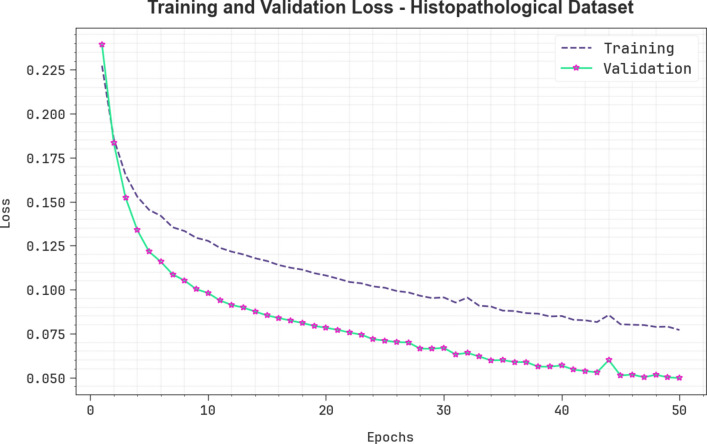
Figure 12 presents the TRA and VLA loss graph of the CVFBJTL-BCD approach on the Histopathological dataset. The loss values are computed for 0–50 epochs. The TRA and VLA accuracy values show a reduced trend, notifying the CVFBJTL-BCD approach’s ability to balance a trade-off between data fitting and generalization. The continual reduction in loss values guarantees the enhanced performance of the CVFBJTL-BCD methodology and tunes the prediction outcomes over time.
Fig. 12.
Loss curve of CVFBJTL-BCD technique on Histopathological dataset.
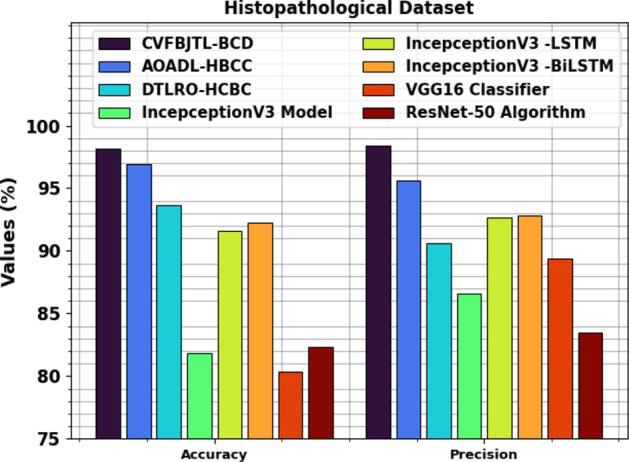
Table 3examines the comparison outcomes of the CVFBJTL-BCD approach on the Histopathological dataset with existing models42,43. Figure 13 illustrates the comparative outcomes of the CVFBJTL-BCD approach on the Histopathological dataset with existing models in terms of and . The outcomes emphasized that the IncepceptionV3, VGG16, and ResNet-50 models have stated worse performance. In the meantime, DTLRO-HCBC, IncepceptionV3 -LSTM, and IncepceptionV3-BiLSTM methodology have got nearer outcomes. At the same time, the AOADL-HBCC process got a higher of 96.95% and of 95.62%. Also, the CVFBJTL-BCD method stated improved performance with the greatest of 98.18% and of 98.38%.
Table 3.
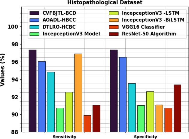
Comparative analysis of CVFBJTL-BCD technique on Histopathological dataset with existing models42,43.
| Histopathological dataset | ||||
|---|---|---|---|---|
| Methods | ||||
| CVFBJTL-BCD | 98.18 | 98.38 | 97.37 | 97.37 |
| AOADL-HBCC | 96.95 | 95.62 | 96.03 | 96.51 |
| DTLRO-HCBC | 93.68 | 90.57 | 94.84 | 93.52 |
| IncepceptionV3 | 81.84 | 86.56 | 90.74 | 91.05 |
| IncepceptionV3 -LSTM | 91.61 | 92.70 | 92.55 | 92.60 |
| IncepceptionV3 -BiLSTM | 92.23 | 92.85 | 96.90 | 91.12 |
| VGG16 Classifier | 80.32 | 89.36 | 89.92 | 90.76 |
| ResNet-50 | 82.33 | 83.46 | 91.06 | 93.40 |
Fig. 13.
and analysis of CVFBJTL-BCD technique on Histopathological dataset.
Figure 14 displays the comparative outcomes of the CVFBJTL-BCD technique on the Histopathological dataset with existing models in terms of and . The results highlighted that the IncepceptionV3, VGG16, and ResNet-50 techniques have stated worse performance. In the meantime, DTLRO-HCBC, IncepceptionV3-LSTM, and IncepceptionV3-BiLSTM techniques have got nearer outcomes. At the same time, the AOADL-HBCC technique got closer of 96.03% and of 96.51%. Also, the CVFBJTL-BCD method stated improved performance with the greatest of 97.37% and of 97.37%.
Fig. 14.
and analysis of CVFBJTL-BCD technique on Histopathological dataset.
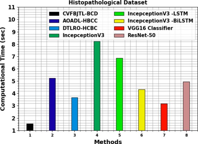
Table 4 and Fig. 15 inspect the computational time (CT) analysis of the CVFBJTL-BCD approach on the Histopathological dataset with existing models. The histopathological dataset analysis reveals diverse computational times for various methods. The CVFBJTL-BCD method performed the fastest at 1.54 s, followed by the VGG16 Classifier at 3.17 s and DTLRO-HCBC at 3.66 s. AOADL-HBCC required 5.23 s, while ResNet-50 took 4.94 s. InceptionV3 had a longer CT of 8.22 s, with its LSTM variant at 6.87 s and the BiLSTM variant at 4.31 s.
Table 4.
CT analysis of CVFBJTL-BCD technique on Histopathological dataset with existing models.
| Histopathological dataset | |
|---|---|
| Methods | CT (sec) |
| CVFBJTL-BCD | 1.54 |
| AOADL-HBCC | 5.23 |
| DTLRO-HCBC | 3.66 |
| IncepceptionV3 | 8.22 |
| IncepceptionV3 -LSTM | 6.87 |
| IncepceptionV3 -BiLSTM | 4.31 |
| VGG16 Classifier | 3.17 |
| ResNet-50 | 4.94 |
Fig. 15.
CT analysis of CVFBJTL-BCD technique on Histopathological dataset with existing models.
The ultrasound dataset contains 780 images under 3 classes, as exposed in Table 5.
Table 5.
Details on dataset.
| Ultrasound dataset | |
|---|---|
| Class | Image count |
| Normal | 133 |
| Benign | 437 |
| Malignant | 210 |
| Total images | 780 |
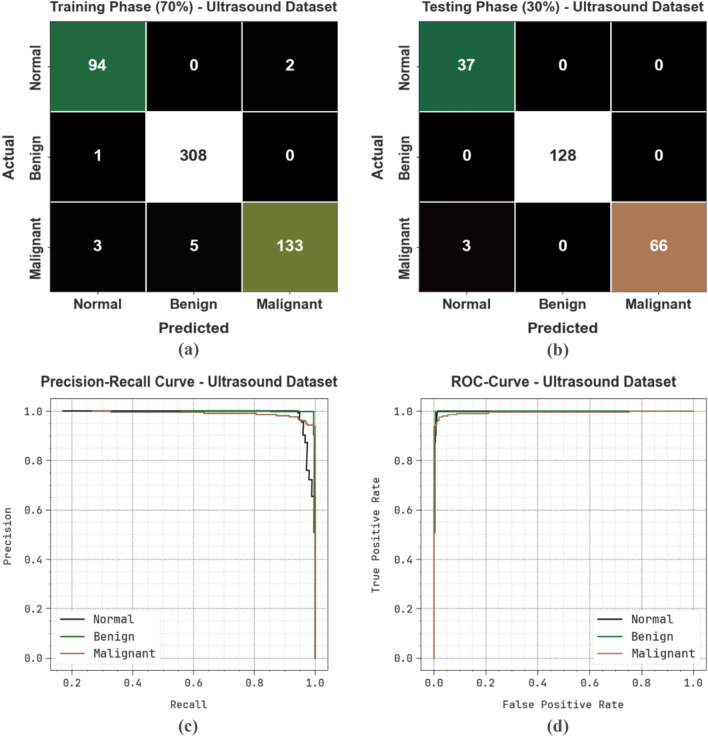
Figure 16 represents the classification results of the CVFBJTL-BCD process on the Ultrasound dataset. Figure 16a-16b displays the confusion matrices with accurate identification and classification of all class labels on a 70:30 TRAP/TESP. Figure 16c represents the PR analysis, indicating maximum performance across all classes. Lastly, Fig. 16d exhibits the ROC analysis, representing efficient outcomes with high ROC values for distinct class labels.
Fig. 16.
Ultrasound Dataset (a-b) Confusion matrices and (c-d) PR and ROC curves.
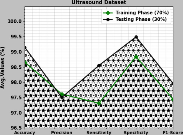
In Table 6 and Fig. 17, the BC detection results of the CVFBJTL-BCD approach are denoted on the Ultrasound dataset. The outcomes reported that the CVFBJTL-BCD approach discriminated adequately between benign and malignant samples. On 70%TRAP, the CVFBJTL-BCD approach provides an average of 98.66%, of 97.61%, of 97.31%, 98.84% and of 97.44%. Also, on 30%TESP, the CVFBJTL-BCD method offers an average of 99.15%, of 97.50%, of 98.55%, 99.49%, and of 97.96%.
Table 6.
BC detection outcomes of CVFBJTL-BCD technique on Ultrasound dataset.
| Class | |||||
|---|---|---|---|---|---|
| TRAP (70%) | |||||
| Normal | 98.90 | 95.92 | 97.92 | 99.11 | 96.91 |
| Benign | 98.90 | 98.40 | 99.68 | 97.89 | 99.04 |
| Malignant | 98.17 | 98.52 | 94.33 | 99.51 | 96.38 |
| Average | 98.66 | 97.61 | 97.31 | 98.84 | 97.44 |
| TESP (30%) | |||||
| Normal | 98.72 | 92.50 | 100.00 | 98.48 | 96.10 |
| Benign | 100.00 | 100.00 | 100.00 | 100.00 | 100.00 |
| Malignant | 98.72 | 100.00 | 95.65 | 100.00 | 97.78 |
| Average | 99.15 | 97.50 | 98.55 | 99.49 | 97.96 |
Fig. 17.
Average of CVFBJTL-BCD technique on Ultrasound dataset.
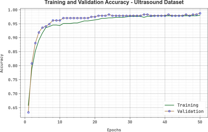
Figure 18 shows the TRA and VLA accuracy outcomes of the CVFBJTL-BCD methodology on the ultrasound dataset. The accuracy values are computed for 0–50 epochs. The figure emphasizes that the TRA and VLA accuracy values are rising, indicating the CVFBJTL-BCD methodology’s capability with improved performance over several iterations. Additionally, the training and validation accuracy remain closer over the epochs, indicating minimal overfitting and enhancing the CVFBJTL-BCD approach’s performance, guaranteeing consistent prediction on unseen samples.
Fig. 18.
curve of CVFBJTL-BCD technique on Ultrasound dataset.
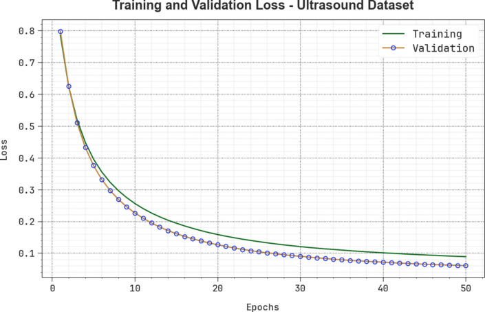
Figure 19 demonstrates the TRA and VLA loss graph of the CVFBJTL-BCD approach on the Ultrasound dataset. The loss values are computed for 0–50 epochs. The TRA and VLA accuracy values show a lower trend, notifying the CVFBJTL-BCD approach’s ability to balance a trade-off between data fitting and generalization. The continual reduction in loss values guarantees the enhanced performance of the CVFBJTL-BCD method and tunes the prediction results over time.
Fig. 19.
Loss curve of CVFBJTL-BCD technique on Ultrasound dataset.
Table 7 examines the comparison results of the CVFBJTL-BCD methodology on the Ultrasound dataset with existing models. Figure 20 exhibits the comparative outcomes of the CVFBJTL-BCD approach on the Ultrasound dataset with existing models in terms of and . The results highlighted that the CNN-VGG16, CNN-VGG19, CNN-Resnet10, CNN-Densnet121, and CNN-Densnet161 methods have stated worse performance. Meanwhile, the EDLCDS-BCDC and ODTLD-CABCC methodologies have yielded nearer outcomes. Also, the CVFBJTL-BCD model stated improved performance with the greatest of 99.15% and of 97.50%.
Table 7.
Comparative analysis of CVFBJTL-BCD technique on Ultrasound dataset with existing models.
| Ultrasound dataset | ||||
|---|---|---|---|---|
| Methods | ||||
| CNN-VGG16 | 91.15 | 85.72 | 90.42 | 87.32 |
| CNN-VGG19 | 92.80 | 88.54 | 95.51 | 94.50 |
| CNN-Resnet101 | 92.06 | 91.32 | 96.75 | 93.72 |
| CNN-Densnet121 | 91.10 | 89.51 | 94.73 | 94.39 |
| CNN-Densnet161 | 88.49 | 83.82 | 96.42 | 95.59 |
| EDLCDS-BCDC | 97.40 | 95.99 | 98.69 | 95.39 |
| ODTLD-CABCC | 98.96 | 98.49 | 99.24 | 97.36 |
| CVFBJTL-BCD | 99.15 | 98.55 | 99.49 | 97.50 |
Fig. 20.
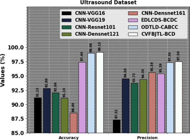
and analysis of CVFBJTL-BCD technique on Ultrasound dataset.
Figure 21 represents the comparative results of the CVFBJTL-BCD method on the Ultrasound dataset with existing models in terms of and . The results emphasized that the CNN-VGG16, CNN-VGG19, CNN-Resnet10, CNN-Densnet121, and CNN-Densnet161 processes have stated worse performance. Meanwhile, the EDLCDS-BCDC and ODTLD-CABCC approaches have yielded nearer outcomes. Also, the CVFBJTL-BCD methodology indicated improved performance with the greatest and of 99.49%.
Fig. 21.
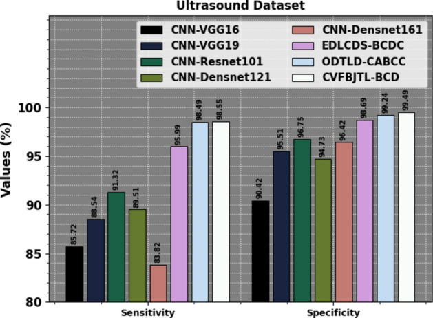
and analysis of CVFBJTL-BCD technique on Ultrasound dataset.
Table 8 and Fig. 22 investigate the CT analysis of the CVFBJTL-BCD methodology on the Ultrasound dataset with existing models. The ultrasound dataset analysis exhibits varying CTs for diverse approaches: CNN-VGG16 took 11.75 s, CNN-VGG19 was faster at 6.52 s, while CNN-Resnet101 required 12.58 s. Other methods comprise CNN-Densnet121 at 14.21 s, CNN-Densnet161 at 13.14 s, EDLCDS-BCDC at 10.33 s, and ODTLD-CABCC at 10.49 s. On the contrary, the CVFBJTL-BCD method attained the shortest CT of 4.96 s.
Table 8.
CT evaluation of CVFBJTL-BCD approach on Ultrasound dataset with existing methods.
| Ultrasound dataset | |
|---|---|
| Methods | Computational time (sec) |
| CNN-VGG16 | 11.75 |
| CNN-VGG19 | 6.52 |
| CNN-Resnet101 | 12.58 |
| CNN-Densnet121 | 14.21 |
| CNN-Densnet161 | 13.14 |
| EDLCDS-BCDC | 10.33 |
| ODTLD-CABCC | 10.49 |
| CVFBJTL-BCD | 4.96 |
Fig. 22.
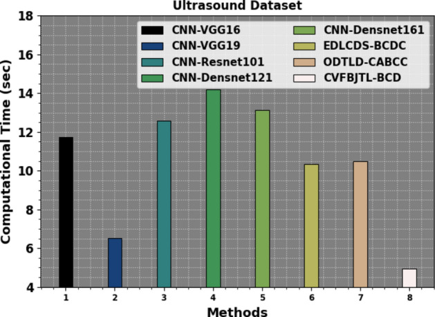
CT evaluation of the CVFBJTL-BCD technique on Ultrasound dataset with existing methods.
Conclusion
This research proposes a new CVFBJTL-BCD technique using multi-modality medical imaging. The presented CVFBJTL-BCD technique gets the perceptions of feature fusion and DL models for effectively detecting and identifying BC diagnosis. Primarily, the presented CVFBJTL-BCD technique applies GF for the noise removal process. Next, the CVFBJTL-BCD technique uses a fusion-based joint TL process comprising three models, namely DenseNet201, InceptionV3, and MobileNetV2. For the classification of BC diagnosis, the SAE model is exploited. Eventually, the HHOA is utilized to select parameters involved in the SAE model optimally. To demonstrate the improved results of the CVFBJTL-BCD methodology, a wide series of experimentations are performed on two benchmark datasets. The comparative analysis of the CVFBJTL-BCD technique portrayed a superior accuracy value of 98.18% and 99.15% over existing methods under Histopathological and Ultrasound datasets. The limitations of the CVFBJTL-BCD technique encompass the reliance on specific datasets that may not fully represent the diversity of breast tumour types and imaging conditions, which can hinder the generalizability of outcomes. Furthermore, discrepancies in imaging equipment and protocols may present biases affecting diagnostic accuracy. Future work may expand the datasets to include a broader range of tumour types and imaging modalities, incorporating ultrasound with MRI or histopathological data to improve diagnostic precision. Exploring advanced DL and optimization models could enhance feature extraction and classification performance. Finally, developing real-time analysis capabilities and user-friendly interfaces will facilitate clinical adoption and support improved decision-making in BC diagnosis.
Author contributions
Iniyan S: Conceptualization, methodology development, experiment, formal analysis, investigation, writing. M. Senthil Raja: Formal analysis, investigation, validation, visualization, writing. R. Poonguzhali: Formal analysis, review and editing. A Vikram : Methodology, investigation. Janjhyam Venkata Naga Ramesh: Review and editing. Sachi Nandan Mohanty: Discussion, review and editing. Khasim Vali Dudekula: Conceptualization, methodology development, investigation, supervision, review and editing. All authors have read and agreed to the published version of the manuscript.
Data availability
The data that support the findings of this study are openly available in the Kaggle repository at https://web.inf.ufpr.br/vri/databases/breast-cancer-histopathological-database-breakhis/ [40].
Declarations
Competing interests
The authors declare that they have no conflict of interest. The manuscript was written with the contributions of all authors, and all authors have approved the final version.
Ethics approval
This article does not contain any studies with human participants performed by any of the authors.
Consent to participate
Not applicable.
Informed consent
Not applicable.
Footnotes
Publisher’s note
Springer Nature remains neutral with regard to jurisdictional claims in published maps and institutional affiliations.
References
- 1.Boumaraf, S., Liu, X., Zheng, Z., Ma, X. & Ferkous, C. A new transfer learning based approach to magnification dependent and independent classification of breast cancer in histopathological images. Biomed. Signal Process. Control63, 102192 (2021). [Google Scholar]
- 2.Bose, S.; Garg, A.; Singh, S.P. Transfer Learning for Classification of Histopathology Images of Invasive Ductal Carcinoma in Breast. In Proceedings of the 2022 3rd International Conference on Electronics and Sustainable Communication Systems (ICESC), Coimbatore, India, 17–19 August 2022; pp. 1039–1044.
- 3.Ahmad, N., Asghar, S. & Gillani, S. A. Transfer learning-assisted multi-resolution breast cancer histopathological images classification. Vis. Comput.38, 2751–2770 (2021). [Google Scholar]
- 4.Issarti, A., Consejo, M., Jiménez-García, S., Hershko, C. & Koppen, J. J. Rozema, Computer aided diagnosis for suspect keratoconus detection. Comput. Biol. Med.109, 33–42. 10.1016/j.compbiomed.2019.04.024 (2019). [DOI] [PubMed] [Google Scholar]
- 5.Habib, M. et al. Detection of microaneurysms in retinal images using an ensemble classifier. Informat. Med. Unlock.9, 44–57 (2017). [Google Scholar]
- 6.Nazir, T. et al. Diabetic retinopathy detection through novel tetragonal local octa patterns and extreme learning machines. Artif. Intell. Med.99, 101695 (2019). [DOI] [PubMed] [Google Scholar]
- 7.Ahmad, H.M.; Ghuffar, S.; Khurshid, K. Classification of breast cancer histology images using transfer learning. In Proceedings of the 2019 16th International Bhurban Conference on Applied Sciences and Technology (IBCAST), Islamabad, Pakistan, 8–12 January 2019; pp. 328–332.
- 8.Alzubaidi, L. et al. Optimizing the performance of breast cancer classification by employing the same domain transfer learning from hybrid deep convolutional neural network model. Electronics9, 445 (2020). [Google Scholar]
- 9.Tsiknakis, N. et al. Deep learning for diabetic retinopathy detection and classification based on fundus images: A review. Comput. Biol. Med.135, 104599 (2021). [DOI] [PubMed] [Google Scholar]
- 10.Ai, Z. et al. DR-IIXRN : Detection algorithm of diabetic retinopathy based on deep ensemble learning and attention mechanism. Front. Neuroinform.15, 778552. 10.3389/fninf.2021.778552 (2021). [DOI] [PMC free article] [PubMed] [Google Scholar]
- 11.Sushanki, S., Bhandari, A. K. & Singh, A. K. A review of computational methods for breast cancer detection in ultrasound images using multi-image modalities. Archives of Computational Methods in Engineering31(3), 1277–1296 (2024). [Google Scholar]
- 12.Abdullakutty, F., Akbari, Y., Al-Maadeed, S., Bouridane, A. and Hamoudi, R., 2024. Advancing Histopathology-Based Breast Cancer Diagnosis: Insights into Multi-Modality and Explainability. arXiv preprint arXiv:2406.12897.
- 13.Oyelade, O. N., Irunokhai, E. A. & Wang, H. A twin convolutional neural network with a hybrid binary optimizer for multi-modal breast cancer digital image classification. Scientific Reports14(1), 692 (2024). [DOI] [PMC free article] [PubMed] [Google Scholar]
- 14.Hu, H., Liang, W., Zou, X. and Zou, X., 2024, July. Graph Convolutional Networks Based Multi-modal Data Integration for Breast Cancer Survival Prediction. In International Conference on Intelligent Computing (pp. 85–98). Singapore: Springer Nature Singapore.
- 15.Yang, X. et al. Triple-attention interaction network for breast tumor classification based on multi-modality images. Pattern Recognition139, 109526 (2023). [Google Scholar]
- 16.Guo, D. et al. A multi-modal breast cancer diagnosis method based on Knowledge-Augmented Deep Learning. Biomedical Signal Processing and Control90, 105843 (2024). [Google Scholar]
- 17.Zhang, J., Chen, Q., Zhou, L., Cui, Z., Gao, F., Li, Z., Feng, Q. and Shen, D., 2023, October. MoSID: Modality-specific information disentanglement from multi-parametric MRI for breast tumor segmentation. In MICCAI Workshop on Cancer Prevention through Early Detection (pp. 94–104). Cham: Springer Nature Switzerland.
- 18.Yan, P., Gong, W., Li, M., Zhang, J., Li, X., Jiang, Y., Luo, H. and Zhou, H., 2024. TDF-Net: Trusted Dynamic Feature Fusion Network for breast cancer diagnosis using incomplete multi-modal ultrasound. Information Fusion, p.102592.
- 19.Karthik, A. et al. Ensemble-based multi-modal medical imaging fusion for tumor segmentation. Biomedical Signal Processing and Control96, 106550 (2024). [Google Scholar]
- 20.Atrey, K., Singh, B. K. & Bodhey, N. K. Integration of ultrasound and mammogram for multi-modal classification of breast cancer using hybrid residual neural network and machine learning. Image and Vision Computing145, 104987 (2024). [Google Scholar]
- 21.Subaar, C. et al. Investigating the detection of breast cancer with deep transfer learning using ResNet18 and ResNet34. Biomedical Physics & Engineering Express10(3), 035029 (2024). [DOI] [PubMed] [Google Scholar]
- 22.Chi, J., Chen, J.H., Wu, B., Zhao, J., Wang, K., Yu, X., Zhang, W. and Huang, Y., 2024. A Dual-Branch Cross-Modality-Attention Network for Thyroid Nodule Diagnosis Based on Ultrasound Images and Contrast-Enhanced Ultrasound Videos. IEEE Journal of Biomedical and Health Informatics. [DOI] [PubMed]
- 23.Li, C. et al. Segmentation prompts classification: A nnUNet-based 3D transfer learning framework with ROI tokenization and cross-task attention for esophageal cancer T-stage diagnosis. Expert Systems with Applications258, 125067 (2024). [Google Scholar]
- 24.Rahman, M. M., Khan, M. S. I. & Babu, H. M. H. BreastMultiNet: A multi-scale feature fusion method using deep neural network to detect breast cancer. Array16, 100256 (2022). [Google Scholar]
- 25.Hasan, M. M. et al. FP-CNN: Fuzzy pooling-based convolutional neural network for lung ultrasound image classification with explainable AI. Computers in Biology and Medicine165, 107407 (2023). [DOI] [PubMed] [Google Scholar]
- 26.Hossain, M. M. et al. Covid-19 detection from chest ct images using optimized deep features and ensemble classification. Systems and Soft Computing6, 200077 (2024). [Google Scholar]
- 27.Hasan, M. M., Hossain, M. M., Mia, S., Ahammad, M. S. & Rahman, M. M. A combined approach of non-subsampled contourlet transform and convolutional neural network to detect gastrointestinal polyp. Multimedia Tools and Applications81(7), 9949–9968 (2022). [Google Scholar]
- 28.Hossain, M. M., Rahim, M. A., Bahar, A. N. & Rahman, M. M. Automatic malaria disease detection from blood cell images using the variational quantum circuit. Informatics in Medicine Unlocked26, 100743 (2021). [Google Scholar]
- 29.Mostafiz, R., Uddin, M. S., Jabin, I., Hossain, M. M. & Rahman, M. M. Automatic brain tumor detection from MRI using curvelet transform and neural features. International Journal of Ambient Computing and Intelligence (IJACI)13(1), 1–18 (2022). [Google Scholar]
- 30.Ai, Y., Liu, J., Li, Y., Wang, F., Du, X., Jain, R.K., Lin, L. and Chen, Y.W., 2024. SAMA: A Self-and-Mutual Attention Network for Accurate Recurrence Prediction of Non-Small Cell Lung Cancer Using Genetic and CT Data. IEEE Journal of Biomedical and Health Informatics. [DOI] [PubMed]
- 31.Nakach, F. Z., Zerouaoui, H. & Idri, A. Binary classification of multi-magnification histopathological breast cancer images using late fusion and transfer learning. Data Technologies and Applications57(5), 668–695 (2023). [Google Scholar]
- 32.Mukhlif, A. A., Al-Khateeb, B. & Mohammed, M. Classification of breast cancer images using new transfer learning techniques. Iraqi Journal For Computer Science and Mathematics4(1), 167–180 (2023). [Google Scholar]
- 33.Mukhlif, A. A., Al-Khateeb, B. & Mohammed, M. A. Incorporating a novel dual transfer learning approach for medical images. Sensors23(2), 570 (2023). [DOI] [PMC free article] [PubMed] [Google Scholar]
- 34.Ali, A. M. & Mohammed, M. A. A comprehensive review of artificial intelligence approaches in omics data processing: evaluating progress and challenges. International Journal of Mathematics, Statistics, and Computer Science2, 114–167 (2024). [Google Scholar]
- 35.Kamil, M. Y. Computer-aided diagnosis system for breast cancer based on the Gabor filter technique. International Journal of Electrical and Computer Engineering (IJECE)10(5), 5235–5242 (2020). [Google Scholar]
- 36.Xiao, J., Gan, C., Zhu, Q., Zhu, Y. & Liu, G. CFNet: Facial expression recognition via constraint fusion under multi-task joint learning network. Applied Soft Computing141, 110312 (2023). [Google Scholar]
- 37.Islam, O., Assaduzzaman, M. and Hasan, M.Z., 2024. An explainable AI-based blood cell classification using optimized convolutional neural network. Journal of Pathology Informatics, p.100389. [DOI] [PMC free article] [PubMed]
- 38.Esmaeiloghli, S., Lima, A. and Sadeghi, B., 2024. Lithium exploration targeting through robust variable selection and deep anomaly detection: An integrated application of sparse principal component analysis and stacked autoencoders. Geochemistry, p.126111.
- 39.Mehrabi, N., Haeri Boroujeni, S.P. and Pashaei, E., 2024. An efficient high-dimensional gene selection approach based on the Binary Horse Herd Optimization Algorithm for biologicaldata classification. Iran Journal of Computer Science, pp.1–31.
- 40.https://web.inf.ufpr.br/vri/databases/breast-cancer-histopathological-database-breakhis/
- 41.Al-Dhabyani, W., Gomaa, M., Khaled, H. & Fahmy, A. Dataset of breast ultrasound images. Data in Brief.28, 104863. 10.1016/j.dib.2019.104863 (2020Feb). [DOI] [PMC free article] [PubMed] [Google Scholar]
- 42.Obayya, M. et al. Hyperparameter optimizer with deep learning-based decision-support systems for histopathological breast cancer diagnosis. Cancers15(3), 885 (2023). [DOI] [PMC free article] [PubMed] [Google Scholar]
- 43.Ragab, M. et al. Optimal deep transfer learning driven computer-aided breast cancer classification using ultrasound images. Expert Systems41(4), e13515 (2024). [Google Scholar]
Associated Data
This section collects any data citations, data availability statements, or supplementary materials included in this article.
Data Availability Statement
The data that support the findings of this study are openly available in the Kaggle repository at https://web.inf.ufpr.br/vri/databases/breast-cancer-histopathological-database-breakhis/ [40].


