Application of multiple linear regression model and long short-term memory with compartmental model to forecast dengue cases in Selangor, Malaysia based on climate variables

Abstract

Despite the implementation of various initiatives, dengue remains a significant public health concern in Malaysia. Given that dengue has no specific treatment, dengue prediction remains a useful early warning mechanism for timely and effective deployment of public health preventative measures. This study aims to develop a comprehensive approach for forecasting dengue cases in Selangor, Malaysia by incorporating climate variables. An ensemble of Multiple Linear Regression (MLR) model, Long Short-Term Memory (LSTM), and Susceptible-Infected mosquito vectors, Susceptible-Infected-Recovered human hosts (SI-SIR) model were used to establish a relation between climate variables (temperature, humidity, precipitation) and mosquito biting rate. Dengue incidence subject to climate variability can then be projected by SI-SIR model using the forecasted mosquito biting rate. The proposed approach outperformed three alternative approaches and expanded the temporal horizon of dengue prediction for Selangor with the ability to forecast approximately 60 weeks ahead with a Mean Absolute Percentage Error (MAPE) of 13.97 for the chosen prediction window before the implementation of the Movement Control Order (MCO) in Malaysia. Extended validation across subsequent periods also indicates relatively satisfactory forecasting performance (with MAPE ranging from 13.12 to 17.09). This research contributed to the field by introducing a novel framework for the prediction of dengue cases over an extended temporal range.

1. Introduction

The mosquito-borne dengue widely spread in countries with tropical and sub-tropical climates. Female mosquitoes of the Aedes species (Ae. aegypti or Ae. albopictus) act as the vectors responsible for transmitting the dengue virus to humans through biting. Approximately half of the world's population is under the threat of dengue (Bhatt et al., 2013; Brady et al., 2012) with about 100–400 million infections each year (Messina et al., 2019). Endemic in Malaysia, dengue has been a public health concern since the 1970s. Despite the implementation of various initiatives and control measures by the Malaysian Government to combat dengue, the disease has continued to increase in frequency and intensity over the past four decades. There is currently no specific treatment for dengue. Although the dengue tetravalent vaccine (live attenuated), Qdenga, was officially launched in Malaysia on June 11, 2024, the cost, estimated to be MYR500 for two doses, is deemed unaffordable to the government and general public. Further, the vaccine does not stop the transmission of dengue virus; it will only reduce the severity of the disease. Hence, dengue control programs focusing on vector eradication, primarily through the use of insecticides and larvicides, and more recently, vector suppression through the release of Wolbachia mosquitoes in localities with a high number of dengue cases (Nazni et al., 2019) remain the primary strategy for controlling dengue transmission.

Dengue prediction models provide a means for stakeholders in the public health system to detect potential outbreaks in advance for timely and strategic implementation of vector control measures. The most common models used are compartmental models, machine learning models and statistical models. Within the realm of compartmental models for disease transmission, the SIR (Susceptible-Infected-Recovered) and SEIR (Susceptible-Exposed-Infected-Recovered) models are the most widely used (Chanprasopchai et al., 2017; Chen, Liu et al., 2022b; Martheswaran et al., 2022). Some variations of these compartmental models included the vector compartments to delineate the disease transmission dynamics between the vector and human (Ramírez-Soto et al., 2023; Wang et al., 2023; Zhu & Xu, 2019). The SI-SIR model captures the interplay between Susceptible-Infected mosquito vectors and Susceptible-Infected-Recovered human hosts, which has been applied by various researchers (Nuraini et al., 2021; Supriatna et al., 2022; Tay et al., 2022). In comparison to the SIR model, the SEIR model includes an ‘exposed’ component, representing individuals who have been infected with the disease but have not yet become infectious. SIR models have been widely used to model infectious diseases including dengue due to their simplicity, enabling researchers to approximate disease behavior by estimating a smaller number of parameters (Mukhsar et al., 2023; Navarro Valencia et al., 2023; Tolles & Luong, 2020).

Over the past several decades, there has been a significant surge in the utilization of tools based on Machine Learning (ML) and Deep Learning (DL) techniques. Both ML and DL are types of artificial intelligence-, that empower computers to learn the crucial features of a given dataset and predict the outcome of a specific event (Balakumar et al., 2022). Various ML algorithms, including decision trees, random forests, support vector machines, artificial neural networks, and gradient boosting algorithms, have been applied for dengue prediction (Batista et al., 2020; Gangula et al., 2023; Hoyos et al. (2021). The advantages and limitations of each algorithm in terms of accuracy, sensitivity, specificity, and area under the curve have also been elaborately discussed and compared. Notably, compared to the traditional techniques of machine learning, deep learning is achieving growing popularity due to its superior abilities such as handling complex patterns and capturing non-linear relationships for predictive forecasting (Shrestha & Mahmood, 2019). In recent years, researchers have increasingly employed deep learning techniques, such as Long Short-Term Memory (LSTM), for dengue prediction. For instance, Doni and Sasipraba (2020) developed a dengue prediction model for India utilizing climatic conditions, and their LSTM-based model achieved forecasting accuracies of over 89% for infection and 81% for death. Saleh and Baiwei (2021) compared the performance of LSTM and Support Vector Regression (SVR) on dengue prediction using weather and climate data and found that LSTM performed better than SVR in capturing the rise and fall trends of dengue.

Statistical models are also widely used for dengue prediction with time series models being the most popular for forecasting dengue outbreaks (Cheng et al., 2020; Dom et al., 2013; Jayaraj et al., 2019; Naher et al., 2022; Thiruchelvam et al., 2021). Time series analysis helps uncover patterns in data by its very nature, which can then be used to predict future data points. Apart from time series models, multiple linear regression (MLR) is another commonly used statistical approach for dengue prediction. For example, Mekparyup et al. (2015) used a multiple linear regression model to forecast the number of monthly dengue fever patients in the Pantong district of Thailand based on meteorological factors, such as temperature, humidity, atmospheric pressure, wind speed, and rainfall. To predict the number of dengue fever incidents in Malang, Indonesia, Anggraeni et al. (2017) employed a modified regression approach, which involves the analysis of the relationship between the number of incidents and various predictor variables using a multiple linear regression model.

Most of the studies on dengue prediction demonstrated the capacity to forecast dengue incidence spanning from 15 days to 4 months (Cheng et al., 2020; Jayaraj et al., 2019; Lu et al., 2024; Nguyen et al., 2022; Nuraini et al., 2021). It is desirable to have a credible forecast of dengue cases for an extended period to allow early detection of changing dengue trends and to allow appropriate mitigation strategies to be planned. Toward this aspiration, this paper proposed a promising approach that integrates compartmental (SI-SIR), deep learning (LSTM), and statistical models (MLR) for forecasting dengue cases. The approach was developed and tested using the dengue and meteorological data available for Selangor, a state in Malaysia with the highest number of dengue cases. In the proposed approach, the mosquito biting rate was first forecasted using the multiple linear regression model, with climate factors serving as the independent variables and biting rate as the dependent variable. Subsequently, the residuals of the multiple linear regression were fitted using the LSTM method. Finally, the forecasted mosquito biting rate was utilized by the SI-SIR model to predict the number of dengue cases.

The dengue and meteorological data used in this study are presented in the next section. A brief overview of the ensemble of methods and tests used is also included. This is followed by the Results section, in which a comprehensive presentation of forecasted dengue cases for the prediction window is given, encompassing outcomes derived from the multiple linear regression model with interaction effect and LSTM method. In addition, the comparative evaluation for the forecasting performance of this proposed approach against three alternative approaches as well as the proposed approach's predictive capabilities across various periods are presented. In the Discussion section, the innovation and limitations of this proposed approach for dengue surveillance and intervention are highlighted. Lastly, the findings of the study are summarized in the Conclusion section.

2. Materials and methods

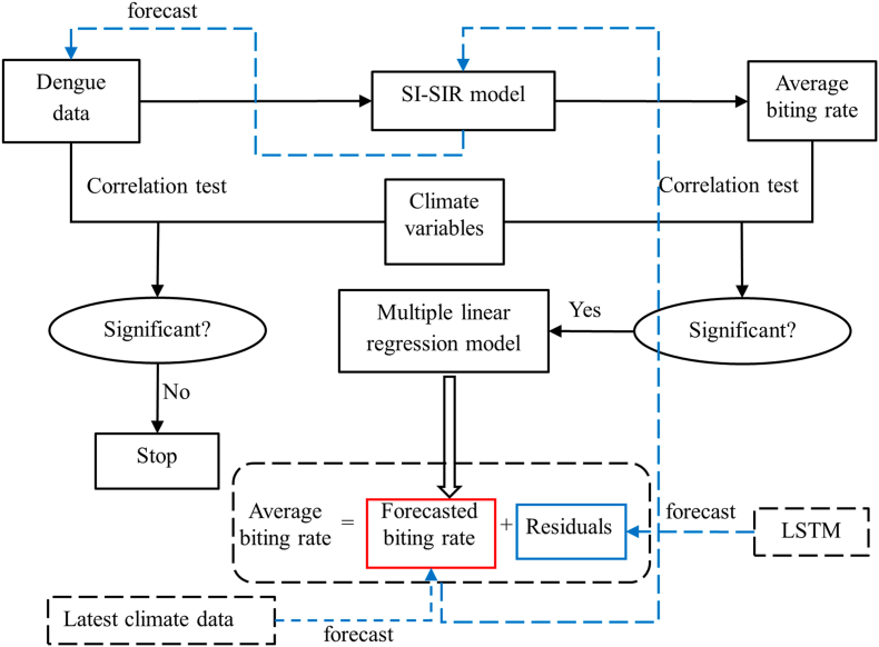
The proposed approach involves a sequence of analyses outlined in Fig. 1. Initially, the biting rate time series was estimated by fitting the simulated results of the SI-SIR model to the dengue data. Subsequently, Pearson correlation coefficients were calculated to assess the linear correlation between climate variables and the average biting rate, as well as between climate variables and dengue cases. The climate variables encompass the data on average temperature, relative humidity, and accumulated precipitation. Based on the results obtained from the Pearson correlation coefficients, an MLR model was constructed to establish a specific relationship between the average biting rate and climate variables. However, certain residuals remained unexplained by the MLR model. To address this, multiresolution analysis was employed to decompose the series of residuals into multiple components, allowing a more detailed examination. Through this decomposition, the time series was further denoised, highlighting the essential information contained in the residuals.

Fig. 1.

Flow chart denoting the sequence of analyses in the proposed approach.

Subsequently, the LSTM model was utilized to train the residual data. This approach further refined the analysis by capturing complex temporal dependencies. The combination of the multiple linear regression model and the LSTM model was then used to forecast the average biting rate. Using the forecasted average biting rate, the dengue cases were ultimately predicted using the SI-SIR model.

2.1. Data

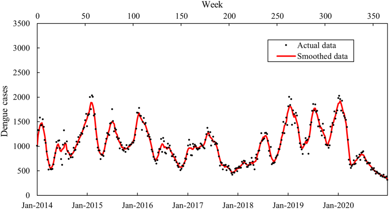
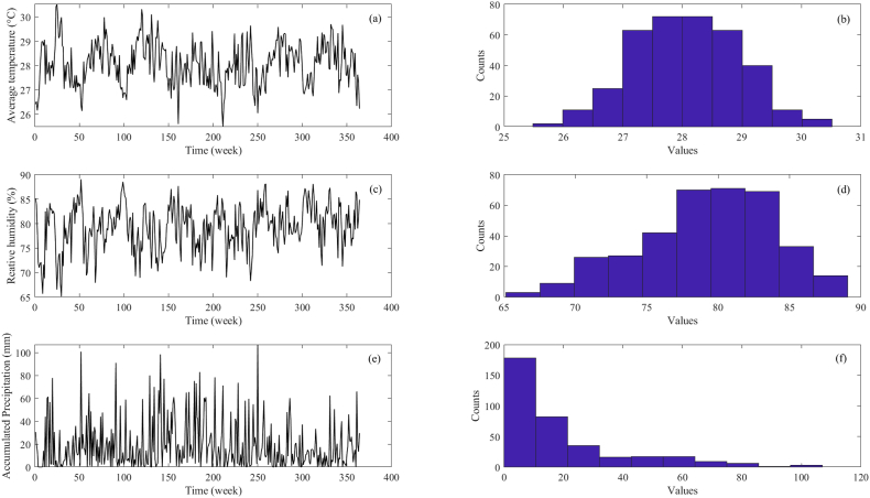
This study utilized the total number of weekly reported dengue cases in Selangor from January 2014 to December 2020 (Fig. 2), obtained from the Ministry of Health Malaysia. The average temperature, relative humidity, and accumulated precipitation used in this study were derived from the daily meteorological data recorded by the Sepang/Kuala Lumpur International Airport monitoring station acquired from MetMalaysia. To align with the weekly dengue data, the average temperature and relative humidity for each week were calculated by computing the arithmetic mean values of the daily temperature and relative humidity. Similarly, the precipitation for each week was determined by summing up the accumulated precipitation during that specific week. The time series and histogram plots of these climate variables are illustrated in Fig. 3. The datasets encompassing dengue cases and climate variables were divided into two distinct segments: the training window and the prediction window. The training window spanned from Week 1 to Week 261 (January 2014 to December 2018), while the prediction window encompassed Week 262 to Week 365 (January 2019 to December 2020). This division allowed us to evaluate the performance of the proposed approach.

Fig. 2.

Actual and smoothed dengue data for Selangor from Jan 2014 to Dec 2020.

Fig. 3.

Time series of average temperature (a), relative humidity (c), accumulated precipitation (e) and the histogram of the data of average temperature (b), relative humidity (d), accumulated precipitation (f) for Selangor from years 2014–2020.

2.2. Method

The methodology in this study comprises five primary components: (i) Estimation of average biting rate in Selangor based on the notified dengue cases from 2014 to 2020 using the SI-SIR model, (ii) Development of a MLR modelusing climatic variables to predict the average biting rate, guided by Pearson correlation coefficients, (iii) Use of multiresolution analysis to examine the residuals of the modeled average biting rate to reveal underlying patterns, (iv) Enhancement of predictive precision by utilizing LSTM on residuals to refine the forecast of average biting rate, and (v) Use of Mean Absolute Error (MAE) and Mean Absolute Percentage Error (MAPE) as evaluative benchmarks to assess predictive accuracy and effectiveness.

2.2.1. SI-SIR model and average biting rate

The Susceptible-Infectious model for the vector infection dynamics and a Susceptible-Infectious-Recovered model for the host population (SI-SIR model) is given in Equation (1). In this compartmental model, the mosquito population is divided into susceptible mosquitoes (V_S) and infected mosquitoes (V_I), while the human population is divided into three compartments, which are susceptible human (H_S), infected human (H_I), and recovered human (H_R). The definition and unit of the parameters in the SI-SIR model are listed in Table 1. Values of the parameters used in the simulation study are also provided together with the source, from which the values were obtained.

$$\begin{array}{l}\frac{d{V}_S}{dt}={\mu }_V{N}_V-B{\beta }_{HV}\frac{H_I}{N_H}{V}_S-{\mu }_V{V}_S\\ \frac{d{V}_I}{dt}=B{\beta }_{HV}\frac{H_I}{N_H}{V}_S-{\mu }_V{V}_I\\ \frac{d{H}_S}{dt}={\mu }_H{N}_H-B{\beta }_{VH}\frac{V_I}{N_H}{H}_S-{\mu }_H{H}_S\\ \frac{d{H}_I}{dt}=B{\beta }_{VH}\frac{V_I}{N_H}{H}_S-{\gamma }_H{H}_I-{\mu }_H{H}_I\\ \frac{d{H}_R}{dt}={\gamma }_H{H}_I-{\mu }_H{H}_R\end{array}$$ (1)

Table 1.

Definition, unit and value of the parameters in the SI-SIR model.

Parameter	Definition	Value	Unit	Source
VS	Susceptible mosquito population	–	capita	–
VI	Infected mosquito population	–	capita	–
HS	Susceptible human population	–	capita	–
HI	Infected human population	–	capita	–
HR	Recovered human population	–	capita	–
NV	Mosquito population	$2\cdot N_H$	capita	–
NH	Human population	$\frac{1}{2}\cdot N_V$	capita	–
μV	Natural mortality rate of mosquito	0.7	week−1	Andraud et al. (2013)
μH	Natural birth/mortality rate of human	$\frac{1}{75\times 52}$	week−1	Andraud et al. (2013)
B	Average biting rate	Curving fitting	week−1	–
βHV	Probability of human-to-mosquito transmission	0.5	–	Lima-Camara et al. (2011)
βVH	Probability of mosquito-to-human transmission	0.75	–	Derouich et al. (2003)
γH	The recovery rate of infected human	0.7	week−1	Andraud et al. (2013)

In previous research, this model was comprehensively discussed by Derouich et al. (2003) and validated by Tay et al. (2022), which was suitable for illustrating the dengue transmission dynamics in Kuala Lumpur and Selangor, Malaysia. The average biting rate can be estimated by fitting the SI-SIR model result to the smoothed dengue data (Tay et al., 2022), using Equation (2).

$$B_i=\left(\frac{{H_I}_{,i+1}-{H_I}_{,i}}{\Delta t}+{\gamma }_H{H}_{I,i}+\mu H_{I,i}\right)\frac{N_H}{{\beta }_{VH}{V}_{I,i}{H}_{S,i}}$$ (2)

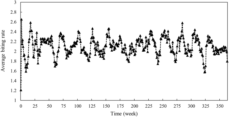
The fitted weekly average biting rate for the period of 365 weeks (Jan 2014–Dec 2020) is illustrated in Fig. 4.

Fig. 4.

Estimated average biting rate by curve fitting using smoothed dengue data.

2.2.2. Pearson correlation coefficient and multiple linear regression model

Before establishing a multiple linear regression model, the relationship between independent (explanatory) variables and the (dependent) response variable should be tested. In this paper, the linear correlation is examined through the Pearson correlation coefficient. Pearson correlation coefficient, r, is a measure of strength of the linear correlation between two data sets (e.g., variables X and Y). The formula of Pearson correlation coefficient is shown in Equation (3). The range of the values are in the closed interval [−1, 1]. The magnitude of the correlation indicates the strength of the linear relationship. If r nears 1, it means there is a positive correlation between the two variables; when r nears −1, it means that the two variables have a negative correlation; while when r = 0, it implies that there is no linear correlation between two variables (Weiss, 2015).

$$r=\frac{\sum _{i=1}^n\left(X_i-\overline{X}\right)\left(Y_i-\overline{Y}\right)}{\sqrt{\sum _{i=1}^n{\left(X_i-\overline{X}\right)}^2}\sqrt{\sum _{i=1}^n{\left(Y_i-\overline{Y}\right)}^2}}$$ (3)

Here, |r| < 0.3 indicates weak linear correlation, 0.3≤|r|≤0.7 indicates moderate linear correlation while |r| > 0.7 indicates strong linear correlation (Akoglu, 2018; Mukaka, 2012; Witte & Witte, 2016). In addition, a t-test (4) is performed to determine whether a Pearson correlation coefficient is statistically significant (Ndako et al., 2020). In this t-test, the null hypothesis is that the correlation coefficient r is close to 0, which means there is insufficient evidence to conclude that the two variables have significant linear correlation. The alternative hypothesis is that the correlation coefficient r is significantly different from 0, which implies that there is a significant linear relationship between the two variables. In practice, when the p-value is less than or equal to 0.05, the null hypothesis will be rejected, indicating the linear correlation. If the p-value is greater than 0.05, the null hypothesis will not be rejected.

$$t=r\cdot \sqrt{\frac{n-2}{1-r^2}}$$ (4)

Multiple linear regression model is a classic statistical technique used to forecast the outcome of a dependent variable based on the values of two or more independent variables. The basic structure of the model is shown in Equation (5).

$$y_i={\beta }_0+{\beta }_1{x}_{i1}+{\beta }_2{x}_{i2}+\dots +{\beta }_p{x}_{ip}+{\epsilon }_i,i=1,2,\dots ,n$$ (5)

Here, subscript i refers to the i-th individual in the population, y_i represents the observed values, which is often called the dependent variable or response variable, x_i is called the independent variable, explanatory variable or regressor, β₀ represents the intercept term while β₁, β₂, …, β_p refer to the regression coefficients and ε_i is called the error term that captures all other factors influencing the dependent variable other than the regressors. In actual application, if there exists dependency between the regressors, this basic multiple linear regression model can also be extended by including an interaction term in the model. This MLR model was employed to establish a relationship between the average mosquito biting rate and climate variables based on a moderate linear association observed between the two. The analysis is presented and discussed in the Results Section. This MLR model is then used to forecast the biting rate based on climate variables, which will be used by the SI-SIR model to predict upcoming dengue cases.

2.2.3. Multiresolution analysis (MRA)

Multiresolution Analysis (MRA) refers to breaking up a signal into components, which produce the original signal exactly when added back together. This term is often associated with wavelets or wavelet packets. By decomposing the signal into multiple components, each with its unique characteristics, MRA realizes the goal of accentuating the information contained within the signal with a high level of detail. In this study, MRA was employed to examine the residuals of the modeled average biting rate, thereby revealing the underlying patterns. Following the construction of a multiple linear regression model with interaction effects, the average biting rate was accounted for by climate variables and residual components, the latter of which are unexplained. Through multiresolution analysis, various components with distinct characteristics can be extracted from the time series of these residuals, which were treated as a signal group. Subsequently, adaptive threshold selection using the principle of Stein's Unbiased Risk Estimate was applied for denoising and enhancing the representation of primary information embedded within the residuals as well as facilitating a more insightful examination of the modeled average biting rate.

2.2.4. LSTM

Long Short-Term Memory (LSTM) is a type of artificial neural network commonly employed in the domains of artificial intelligence and deep learning. As a variant of the recurrent neural network (RNN), LSTM was developed to address the limitation of traditional RNNs (Hochreiter & Schmidhuber, 1997). LSTM model components, including memory blocks, input gate, output gate, and forget gate, are employed to effectively capture long-term dependencies and subtle patterns in sequential data. In this study, after constructing a multiple linear regression model with interaction effects to model the average biting rate, the residuals of this model were subjected to further refinement using LSTM. The LSTM model was trained on the residuals to capture additional temporal patterns and dependencies that may not have been fully accounted for by the regression model. By doing so, the LSTM model can generate more accurate predictions of the residual components of the average biting rate. This process was performed in MATLAB R2022a using Deeping Learning Toolbox (The MathWorksInc, 2022).

2.2.5. Evaluation criteria

Evaluation criteria are designed to assess the accuracy and effectiveness of the model's predictions by analyzing the output values in relation to the input data. For this study, the chosen evaluation criteria are MAE (6) and MAPE (7). MAE is the mean absolute difference between the actual and the forecasted value, while MAPE is the mean absolute percentage difference between the actual and the forecasted value. When utilizing MAE and MAPE as performance assessment metrics, lower MAE and MAPE indicate a superior model performance.

$$MAE=\frac{1}{n}\sum _{i=1}^n\left|y_{actual}-y_{forecasted}\right|$$ (6)

$$MAPE=\frac{1}{n}\sum _{i=1}^n\left|\frac{y_{actual}-y_{forecasted}}{y_{actual}}\right|\cdot 100$$ (7)

3. Results

This section presents the (a) established multiple linear regression model with interaction effect; (b) components of residuals that was decomposed through MRA and the denoised time series of residuals; (c) forecasted dengue cases for the prediction window with multiple linear regression model and the LSTM method; (d) comparison with alternative approaches; (e) forecasting competence of the proposed approach for various prediction periods.

3.1. Multiple linear regression model with interaction effect

The Pearson correlation coefficients between the reported dengue cases and the climate variables (Table 2) indicate a modest linear correlation existing between dengue cases and the considered climate variables. The Pearson correlation coefficient pertaining to dengue cases and relative humidity was calculated to be −0.0899, while the correlation between dengue cases and accumulated precipitation yielded a value of −0.0898. Moreover, the p-values from the t-tests underscored the inability to reject the null hypothesis, signifying a lack of linear correlation between the variables. Although the p-value derived from the t-test suggested a potential linear correlation between dengue cases and temperature, the associated Pearson correlation coefficient merely attained a value of 0.1189. This set of results collectively indicates the challenge in establishing a robust multiple linear regression model between dengue cases and the considered climate variables.

Table 2.

Results of correlation tests among the dengue cases and climate variables.

Correlation	Pearson correlation coefficient	p-value of t-test
Dengue cases & average temperature	0.1189	0.0232
Dengue cases & relative humidity	−0.0899	0.0862
Dengue cases & accumulated precipitation	−0.0898	0.0868

Comparatively, the linear association between the average biting rate and climate variables is higher (Table 3). A moderate negative linear correlation (−0.3128) between the average biting rate and average temperature and a moderate positive linear correlation (0.3778) between the average biting rate and relative humidity are observed. The p-value from the t-test for the correlation between average biting rate and average temperature is 1.06 × 10⁻⁹, while for average biting rate and relative humidity, it is 8.525 × 10⁻¹⁴. Both values are significantly less than 0.05, indicating that the probability of the null hypothesis (which assumes the Pearson correlation coefficient is close to 0) occurring by chance is minimal. Therefore, the null hypothesis can be rejected. These results suggest a statistically significant correlation between the average biting rate and the two climate variables. Further, the Pearson correlation coefficient between average temperature and relative humidity is −0.6932 (Table 4), thereby signifying a robust linear correlation between these two variables. Hence, the inclusion of interaction effects within the framework of a multiple linear regression model is required.

Table 3.

Results of correlation tests among the average biting rate and climate variables.

Correlation	Pearson correlation coefficient	p-value of t-test
Average biting rate & average temperature	−0.3128	1.06 × 10−9
Average biting rate & relative humidity	0.3778	8.525 × 10−14
Average biting rate & accumulated precipitation	0.0356	0.4979

Table 4.

Results of correlation tests among the climate variables.

Correlation	Pearson correlation coefficient	p-value of t-test
Average temperature & relative humidity	−0.6932	<2.2 × 10−16
Average temperature & accumulated precipitation	−0.2448	2.213 × 10−6
Relative humidity & accumulated precipitation	0.1885	0.0003

A weak linear correlation (0.0356) between the average biting rate and accumulated precipitation is also obtained. The underlying causes for this weak correlation may be attributed to intrinsic attributes of the relationship itself or potentially influenced by other contributory factors. Examining the weekly accumulated precipitation data from January 2014 to December 2020, it is observed that approximately 11% of the dataset contains nil values. Typically, nil values for accumulated precipitation can occur in three situations: (1) no precipitation occurred during the observation period, (2) there was precipitation, but the amount was too small for the meteorological station to record, or (3) there was detectable precipitation, but the instrument malfunctioned during the observation period. To account for the effect of precipitation, a multiple linear regression model for cases where the accumulated precipitation value is nil or non-nil is established. The specific formulation is presented in Equations (8), (9), where the average temperature and relative humidity are denoted as T and H, respectively. Additionally, a₀ and A₀ represent the constant term, a₁ and A₁ represent the coefficients for average temperature, a_2, and A₂ represent the coefficients for relative humidity, a_3, and A₃ represent the coefficient for the interaction of average temperature and relative humidity, and e represents the residuals. When the value of accumulated precipitation is nil:

$$b=a_0+a_{1}T+a_{2}H+a_{3}TH+e$$ (8)

When the value of accumulated precipitation is not nil:

$$b=A_0+A_{1}T+A_{2}H+A_{3}TH+e$$ (9)

In order to combine the two equations into a single equation, the values of accumulated precipitation in the dataset are transferred as Boolean variables following the criteria in Equations (10), (11)

$$F=\{\begin{array}{l}1\text{if}\text{accumulative}\text{precipitation}=0\\ 0\text{if}\text{accumulative}\text{precipitation}>0\end{array}$$ (10)

$$M=\{\begin{array}{l}1\text{if}\text{accumulative}\text{precipitation}>0\\ 0\text{if}\text{accumulative}\text{precipitation}=0\end{array}$$ (11)

Then the two equations can be combined as Equation (12).

$$b=\left(a_0+a_{1}T+a_{2}H+a_{3}TH\right)\cdot F+\left(A_0+A_{1}T+A_{2}H+A_{3}TH\right)\cdot M+e=a_{0}F+a_{1}TF+a_{2}HF+a_{3}THF+A_{0}M+A_{1}TM+A_{2}HM+A_{3}THM+e$$ (12)

In this way, a multiple linear regression model with interaction effect is eventually established. By denoting F as x₁, TF as x₂, HF as x₃, THF as x₄, M as x₅, TM as x₆, HM as x₇ and THM as x₈, Equation (12) can be rewritten as Equation (13).

$$\{\begin{array}{l}b=u+e\\ u=a_0{x}_1+a_1{x}_2+a_2{x}_3+a_3{x}_4+A_0{x}_5+A_1{x}_6+A_2{x}_7+A_3{x}_8\end{array}$$ (13)

The values of coefficients in Equation (13) can be estimated after substituting the data of training window (Weeks 1–261). The specific formula is therefore obtained as shown in Equation (14).

$$b=-3.23x_1+0.139x_2+0.058x_3-0.002x_4+0.308x_5+0.002x_6+0.008x_7-0.000078x_8+e$$ (14)

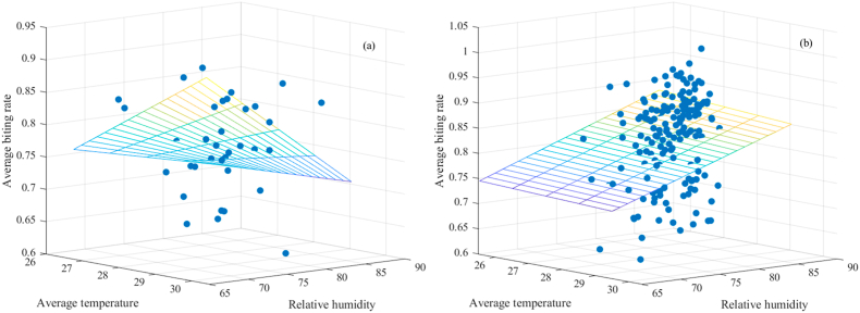
As depicted in Fig. 5, a discrepancy arises in the quantity of data points associated with accumulated precipitation values being nil compared to those where values are not nil. This discrepancy emphasizes a more evident influence of the interplay between average temperature and relative humidity within the context of the multiple linear regression model, particularly when the accumulated precipitation value is nil. However, when the dataset expands in size, this interaction effect tends to substantially diminish, as demonstrated in the scenario involving non-nil accumulated precipitation values.

Fig. 5.

Plotted data (a) when the value of accumulated precipitation is nil and (b) when the value of accumulated precipitation is not nil using the multiple linear regression model with interaction effect.

3.2. Analysis and forecast of the residuals

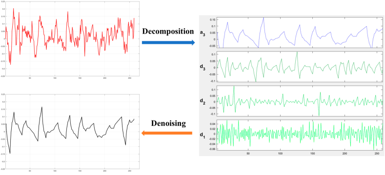
After building the multiple linear regression model with interaction effect, the average biting rate was partly explained by the climate variables. The remaining parts that could not explained by part of u in Equation (13) were reflected in the residuals e. Generally, residuals are important as the magnitude of the residuals could influence the quality of a whole model. In this study, the time series of the residuals of the multiple linear regression model was regarded as a group of signals, the multiresolution analysis was then applied to get the multiple components with different characteristics. In order to highlight the main information contained in the residuals, the time series of the residuals was denoised based on the results of multiresolution analysis. The process of decomposing and denoising the residuals of the average biting rates is shown in Fig. 6. The component of residuals is first decomposed via a multilevel 1-D discrete wavelet transform. Then the decomposition part leads to the denoised residuals through the adaptive threshold selection.

Fig. 6.

Decomposition and denoising of residual components derived from the multiple linear regression model incorporating interaction effects.

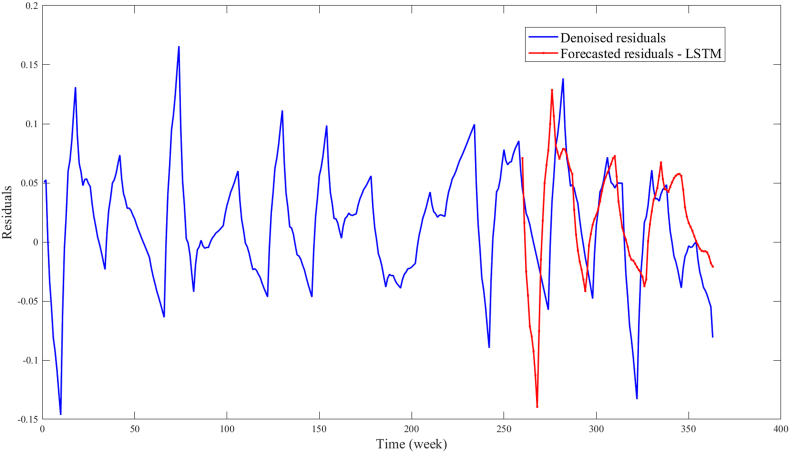
Next, the residuals of the multiple linear regression model with interaction effect were forecasted with the LSTM model. As illustrated in Fig. 7, the general patterns of the residuals can be discerned. However, towards the later part (Weeks 325–365) of the prediction window, there is a noticeable divergence between the projected residual values and the actual trend. This divergence can be attributed to the LSTM's methodology of time series forecasting, which hinges on capturing the underlying temporal dependencies and patterns within the data (Lindemann et al., 2021). When shifts in these patterns occur, the LSTM-generated forecasts may exhibit divergence. This divergence in residual predictions may cause an impact on the anticipated average biting rate within specific intervals (Weeks 325–365), further influencing the prediction of dengue cases. Consequently, an obvious deviation arises between the forecasted and actual trends of dengue cases in the time frame of Weeks 325–365.

Fig. 7.

Forecasted residuals for the prediction window (from Weeks 262–365) of the multiple linear regression model with interaction using LSTM.

3.3. Forecasted dengue cases for the prediction window

The number of dengue cases for the prediction window spanning from Week 262 to Week 365 (January 2019–December 2020) was forecasted to assess the performance of the model. Subsequently, the MAE and MAPE were calculated to evaluate the accuracy of the model's predictions.

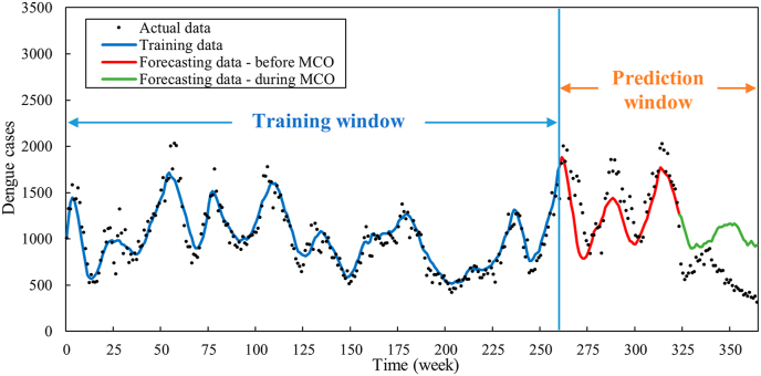
As presented in Fig. 8, the forecasting of dengue cases demonstrates a commendable overall accuracy, with an exception observed in the latter phase of the prediction window, coinciding with the implementation period of the Movement Control Order (MCO) in Malaysia. This deviation in dengue prediction aligns consistently with the outcomes depicted in the forecasted residuals (Fig. 7). It is important to note that an unforeseen event occurred on March 18, 2020, when the Malaysian Government implemented the MCO to curtail the transmission of COVID-19 in Malaysia (Teh et al., 2021). This event had an inadvertent impact on the transmission of dengue, potentially leading to changes in the reported number of dengue cases in 2020. Therefore, we divided the prediction window into two periods: pre-MCO (Weeks 262–324) and post-MCO (Weeks 325–365). As indicated in Table 5, MAE and MAPE were calculated for each temporal interval. Preceding the initiation of the MCO, the predictions exhibited a notably elevated level of accuracy. During this period, both the MAE and MAPE values were significantly lower in comparison to the interval encompassing the MCO's enforcement. Specifically, prior to the MCO, the MAPE was 13.97, whereas during the MCO, the MAPE surged to 87.03. Understandably, the model would not be able to capture the unprecedented change in dengue trend due to the lockdown. But the significant deviation of the reported dengue cases from the predicted number of dengue cases signals a major change in the contributing factors of dengue.

Fig. 8.

Forecasted dengue cases for the prediction window (from week 262 to week 365).

Table 5.

Evaluation criteria (MAE and MAPE) for the prediction window (from week 262 to week 365).

Evaluation criteria	Forecasting periods
	Week 262–324 (Before MCO)	Week 325–365 (During MCO)
MAE	204.36	434.02
MAPE	13.97	87.03

3.4. Comparison with alternative approaches

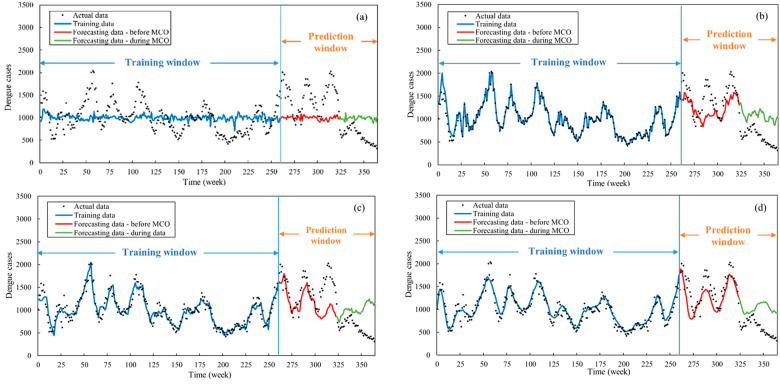
To elucidate the forecasting capability of the proposed approach, its performance is compared to three alternative approaches, namely using (i) only MLR to forecast dengue cases subject to climate variables (Approach A), (ii) only LSTM to forecast dengue cases subject to climate variables (Approach B), and (iii) both MLR and LSTM without associating mosquito biting rate with climate variables (Approach C). The proposed approach, which combines MLR and LSTM and associating mosquito biting rate with climate variables, is referred to as Approach D. The outcome of this comparative exercise is graphically depicted in Fig. 9, while the corresponding MAE and MAPE values are tabled (Table 6).

Fig. 9.

Comparison of the forecasting performance of four approaches: (a) using only MLR to forecast dengue cases subject to climate variables (Approach A), (b) using only LSTM to forecast dengue cases subject to climate variables (Approach B), and (c) using both MLR and LSTM without associating mosquito biting rate with climate variables (Approach C) and (d) using both MLR and LSTM and associating mosquito biting rate with climate variables (Approach D).

Table 6.

Evaluation criteria (MAE and MAPE) of four approaches for the prediction window (from Weeks 262–365).

Approach	MAE		MAPE
	Week 262–324 (Before MCO)	Week 325–365 (During MCO)	Week 262–324 (Before MCO)	Week 325–365 (During MCO)
A	471.77	393.75	29.57	79.41
B	270.80	479.38	17.53	92.36
C	313.85	418.17	20.03	88.28
D	204.36	434.02	13.97	87.03

Prior to the implementation of MCO, Approach A yielded the least favorable results, notably lacking the ability to capture discernible trends in dengue cases. This shortcoming can be attributed to the intrinsic linearity of the MLR framework, which, as established by the weak linear correlation between dengue cases and climate variables (Table 3), rendered it insufficient to yield anticipated predictive accuracy. In the same prediction window, Approaches B and C exhibited commendable capabilities in capturing primary dengue case trends with MAPE values of 17.53 and 20.03, respectively. Notably, Approach D (the proposed approach) outperformed all others with comparably the lowest MAPE value of 13.97.

During the MCO period, none of the approaches, including Approach D, achieved satisfactory forecasting performance (MAPE ranged from 87.03 to 92.36). This discrepancy can be attributed to the substantial disruption induced by the MCO in Malaysia. The measures imposed during the MCO, encompassing restrictions on movement and gatherings, closure of academic and public establishments, and travel limitations, fundamentally altered dengue transmission dynamics. The lockdown perturbed dengue transmission by limiting human movement and geographic spread and reducing time spent in dengue hotspots, thereby reducing vector-host interactions (Ahmad Zaki & Xin, 2023). Consequently, the mathematical models were inadequate to foresee the unforeseeable events engendered by the COVID-19 pandemic and the MCO.

3.5. Forecasting competence for various prediction periods

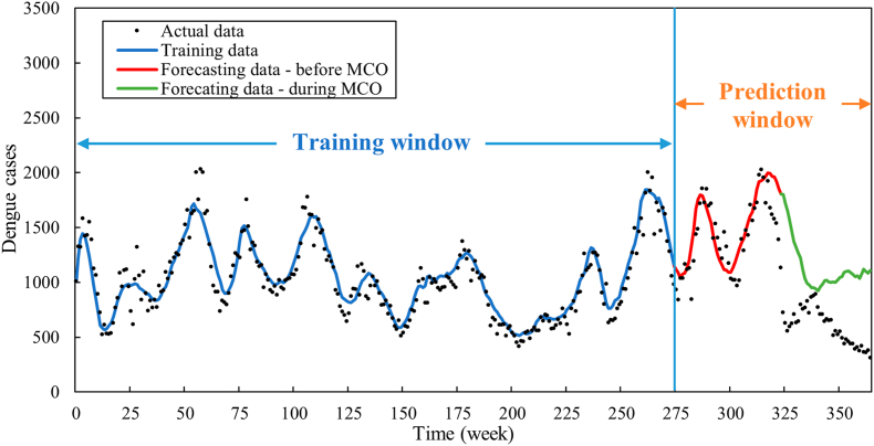
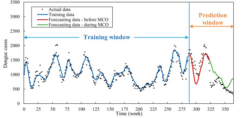
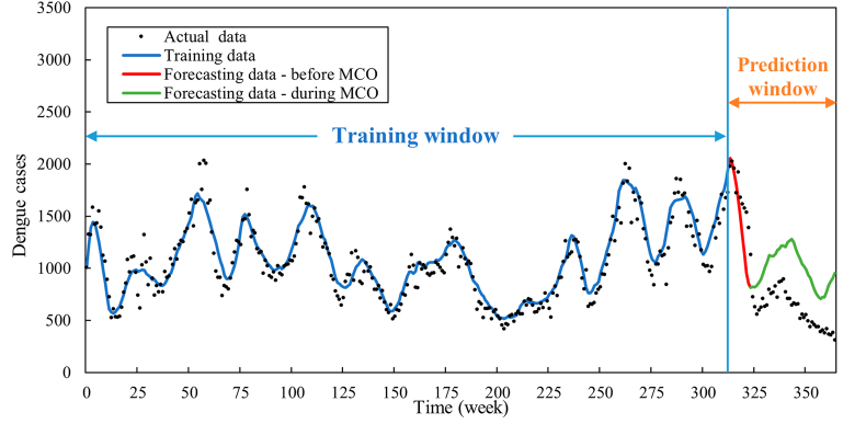
In addition to the predictions spanning Weeks 262–365 (January 2019 to December 2020), the evaluation was extended to three additional prediction intervals, namely (i) Weeks 276–365, (ii) Weeks 290–365, and (iii) Weeks 314–326. Fig. 10, Fig. 11, Fig. 12 portray the predictive outcomes for these periods, respectively, while the corresponding MAE and MAPE values are listed in Table 7, Table 8, Table 9.

Fig. 10.

Forecasted dengue cases for Weeks 276–365.

Fig. 11.

Forecasted dengue cases for Weeks 290–365.

Fig. 12.

Forecasted dengue cases for Weeks 314–365.

Table 7.

Evaluation criteria (MAE and MAPE) for Weeks 276–365.

Evaluation criteria	Forecasting periods
	Week 276–324 (Before MCO)	Week 325–365 (During MCO)
MAE	169.03	539.46
MAPE	13.12	105.58

Table 8.

Evaluation criteria (MAE and MAPE for Weeks 290–365.

Evaluation criteria	Forecasting periods
	Week 290–324 (Before MCO)	Week 325–365 (During MCO)
MAE	237.75	274.56
MAPE	17.09	52.26

Table 9.

Evaluation criteria (MAE and MAPE for Weeks 314–365.

Evaluation criteria	Forecasting periods
	Week 314–324 (Before MCO)	Week 325–365 (During MCO)
MAE	256.94	398.02
MAPE	16.93	37.38

All prediction intervals exhibit a commendable ability to capture primary trends preceding the MCO. Notably, predictive accuracy stays at a relatively stable level as the training dataset is augmented. The MAE fluctuates from 169.03 to 256.94, and the MAPE ranges from 13.12 to 17.09. However, MAE and MAPE values remain relatively elevated for all prediction intervals during the MCO (post-week 324). This observation underscores an intrinsic limitation wherein mathematical models are predisposed to falter when confronted with abrupt deviations that defy historical patterns. The occurrence of a drastic decline in dengue cases in 2020 during the lockdown accentuates this phenomenon, underscoring that mathematical and statistical models are contingent upon past patterns and may falter when confronted with unforeseen deviations.

4. Discussion

Dengue forecasting models will markedly enhance the preparedness of the health systems, especially in the changing climate, by improving dengue surveillance and intervention capabilities. The forecasts help identify the most likely period of disease outbreak so that intervention plans can be put in place to mitigate the outbreak. In addition, when unforeseen events, which are unrelated to climate change, significantly affect dengue cases, the disparity between data trends and forecasting results serves as a reminder for decision-makers to closely monitor the emerging dengue trends and promptly conduct investigations to pinpoint the cause. Towards these aspirations, the approach proposed in this study combines the MLR, LSTM, and SI-SIR models to enable the forecast of dengue cases subject to climate variables for an extended period. In this approach, the dengue cases were projected using the predicted biting rates since statistical analyses revealed the relationship between the biting rates and climate variables. Unlike many statistical models (Mussumeci & Codeço Coelho, 2020; Mendoza, 2023) developed based on direct fitting to the number of dengue cases, the proposed approach would allow the determination of dengue mitigation measures required to combat the surge in dengue cases in a changing climate via the SI-SIR model. The rationale for incorporating the biting rate lies in its closer biological relationship with mosquito behavior, which is climate-sensitive. By modeling mosquito biting rates, we account for the intermediary dynamics between climate and disease transmission, enabling more detailed insights into how climate conditions drive changes in dengue risk. While there is some benefit to fitting the model directly to case numbers, our method offers a more dynamic understanding of climate's role in shaping transmission patterns, leading to better-informed interventions.

As a commonly used compartmental model for disease modeling (Nuraini et al., 2021; Zhu et al., 2020), the SI-SIR model comprises the susceptible and infectious compartments for mosquitoes and the susceptible, infectious, and recovered compartments for humans. This compartmentalization not only allows a better representation of the biological processes involved in dengue transmission, where a mosquito/human is allowed to move from one compartment to another at an appropriate rate, but also offers a flexible framework to explore interventions such as mosquito intervention measures. The choice of parameters in the SI-SIR model is grounded in empirical studies validating their relevance for dengue transmission in Malaysia. Particularly, the effectiveness of the SI-SIR model in simulating dengue dynamics in Kuala Lumpur and Selangor, Malaysia, has been validated by Tay et al. (2022), making it a suitable framework for this study.

Existing models largely use only either the stand-alone compartmental model (Lin et al., 2023; Lizarralde-Bejarano et al., 2022), which is limited in its ability to project dengue cases in a changing climate, or the statistical model (Chen, Li et al., 2022a; Ismail et al., 2022), which does not allow further analysis of the intervention measures. In this respect, the proposed approach is deemed promising not only in forecasting dengue cases in a changing climate for an extended period but also in having an adaptable framework for examining the efficiency of dengue intervention measures, aiding the development of better preparedness and response strategies. For instance, mosquito fogging can be conducted irregularly prior to the next dengue outbreak, temporarily suppressing populations of susceptible and infected mosquitoes and consequently leading to a reduction in dengue cases. Additionally, novel intervention strategies such as the release of Wolbachia-infected mosquitoes can be explored further by expanding the compartmental model in our proposed approach to incorporate a more complex system, containing both Wolbachia-carrying and Wolbachia-free vectors.

In contrast to existing research in the domain of dengue case prediction in Malaysia, this study introduces several innovative facets. Firstly, a comparative analysis is performed, highlighting the superior accuracy of our proposed approach in comparative with other methodologies. Secondly, the integration of multiresolution analysis and deep learning techniques to forecast residual terms within a multiple linear regression framework enhances predictive capabilities, a novel endeavor within the context of dengue forecasting in Malaysia. Lastly, this study extends the prediction horizon beyond the conventional short-term forecasts (often 1–4 weeks in advance) to a longer-term forecast (approximately 20–60 weeks in advance) with reliable accuracy (MAPE ranging from 13.12 to 17.09). This feature is distinctive in the landscape of dengue prediction research.

Some noteworthy limitations of this study are also acknowledged. Firstly, the unavailability of comprehensive mosquito data necessitated reliance on the average biting rate as a proxy for climate-mediated effects on mosquito populations, a simplification that may warrant further scrutiny from a biological standpoint. Secondly, the adoption of the SI-SIR model, while robust, is confined to basic compartments and a single dengue serotype, warranting future refinements for comprehensive modeling. Further, while a moderate negative linear correlation between the average biting rate and temperature and a moderate positive correlation between biting rate and relative humidity was observed, these relationships may not fully capture the complexities of mosquito behavior in response to climatic factors. The linear model may oversimplify interactions, such as the reduction in mosquito activity at higher temperatures due to heat stress or changes in biting rate with varying levels of humidity. The model appears to work reasonably for Selangor because the site experiences relatively stable temperatures and humidity that vary within a narrow range throughout the year. This may limit the applicability of this approach to regions with less extreme or variable climatic conditions. Lastly, the inherent challenge of parameter tuning in deep learning, given the lack of universal standards, remains a prevalent concern within the field.

Despite these limitations, the combination of traditional statistical models with advanced machine learning techniques offers a promising approach to improving dengue forecasting and public health preparedness. Notably, deep learning models such as the LSTM model hold a significant role in improving public health as tools for predictive analytics, among others. LSTM models are good at capturing long temporal dependencies, making them highly useful for time series forecasting in complex and non-linear patterns, such as those found in climate and disease-related data. In this study, the LSTM model addresses residuals unexplained by the MLR model, suggesting that traditional statistical methods may not fully capture all variations driven by external temporal factors. This demonstrates that advanced machine learning models can complement traditional methods to better anticipate fluctuations in future trends, leading to better forecasts of dengue outbreaks and the progression and assessment of public health interventions. The predictive capabilities of LSTM can improve the identification of outbreak patterns, providing better lead times for intervention planning. This contributes to a more robust public health preparedness, allowing authorities to respond proactively to forecasted dengue trends, thereby reducing the potential burden on healthcare systems. Future research should explore threshold models to better account for potential nonlinearities in mosquito behavior in relation to climate variables. A richer corpus of notified dengue cases and climate data shall be obtained to recalibrate the model, accommodating the transformed dynamics post-COVID-19. A longitudinal exploration of dengue trends amidst evolving climatic conditions is poised to offer valuable insights.

5. Conclusion

The ensemble approach of the MLR model, LSTM, and SI-SIR model not only demonstrated the capacity to forecast dengue cases for Selangor, Malaysia with a lead time of approximately 20–60 weeks, but also displays its competence in predicting cases with noteworthy precision. Dengue and meteorological data from January 2014 to December 2018 (Weeks 1–261) were utilized for model training/calibration purpose while dengue cases were predicted from January 2019 to December 2020 (Weeks 262–365). During the period preceding the implementation of the MCO, the MAE and MAPE of the predictions were markedly lower, measuring 204.36 and 13.97, respectively. Further, in comparison with three alternative approaches, the proposed approach recorded the lowest MAE and MAPE for the weeks preceding and during MCO. The MAPE of the predictions by the proposed approach across various validation periods (Weeks 276–365, Weeks 290–365, and Weeks 314–365) was consistently low, ranging from 13.12 to 17.09 for the period preceding the implementation of MCO. However, during the period coinciding with the implementation of the MCO, the MAE and MAPE of the predictions experienced a relative increase. This suggests that the proposed approach would not be able to capture well the unprecedented deviation of data trend.

CRediT authorship contribution statement

Xinyi Lu: Writing – review & editing, Writing – original draft, Visualization, Validation, Software, Methodology, Investigation, Formal analysis. Su Yean Teh: Writing – review & editing, Writing – original draft, Supervision, Resources, Project administration, Methodology, Funding acquisition, Data curation, Conceptualization. Chai Jian Tay: Writing – review & editing, Writing – original draft, Supervision, Resources, Investigation, Funding acquisition. Nur Faeza Abu Kassim: Writing – review & editing, Resources, Methodology, Investigation. Pei Shan Fam: Writing – review & editing, Supervision, Software, Methodology. Edy Soewono: Writing – review & editing, Resources, Methodology.

Data availability

The dengue and meteorological data that support the findings of this study are available from Malaysian Ministry of Health (MOH) and MetMalaysia, respectively, but restrictions apply to the availability of these data, which were used under licence for the current study, and so are not publicly available. Dengue data are however available from MOH upon application to National Medical Research Register. Meteorological data are available from the corresponding author on reasonable request.

Declaration of competing interest

The authors declare that they have no known competing financial interests or personal relationships that could have appeared to influence the work reported in this paper.

Handling Editor: Dr Yiming Shao

References

- Ahmad Zaki R., Xin N.Z. Dengue trend during COVID-19 pandemic in Malaysia. Asia-Pacific Journal of Public Health. 2023;35(1):62–64. doi: 10.1177/10105395221134655. [DOI] [PMC free article] [PubMed] [Google Scholar]
- Akoglu H. User's guide to correlation coefficients. Turkish Journal of Emergency Medicine. 2018;18(3):91–93. doi: 10.1016/j.tjem.2018.08.001. [DOI] [PMC free article] [PubMed] [Google Scholar]
- Andraud M., Hens N., Beutels P. A simple periodic-forced model for dengue fitted to incidence data in Singapore. Mathematical Biosciences. 2013;244(1):22–28. doi: 10.1016/j.mbs.2013.04.001. [DOI] [PubMed] [Google Scholar]
- Anggraeni W., Nurmasari R., Riksakomara E., Samopa F., Wibowo R.P., Condro T.L., Pujiadi Modified regression approach for predicting number of dengue fever incidents in Malang Indonesia. Procedia Computer Science. 2017;124:142–150. [Google Scholar]
- Balakumar M., Vontela H.R., Shinde V.V., Kulshrestha V., Mishra B., Aduri R. Dengue outbreak and severity prediction: Current methods and the future scope. VirusDisease. 2022;33(2):125–131. doi: 10.1007/s13337-022-00767-x. [DOI] [PMC free article] [PubMed] [Google Scholar]
- Batista E.D., Bublitz F.M., Araújo W.C., Lira R.V. Dengue prediction through machine learning and deep learning: A scoping review protocol. Research Square. 2020 doi: 10.21203/rs.3.rs-95498/v1. [DOI] [Google Scholar]
- Bhatt S., Gething P.W., Brady O.J., Messina J.P., Farlow A.W., Moyes C.L., Drake J.M., Brownstein J.S., Hoen A.G., Sankoh O., Myers M.F., George D.B., Jaenisch T., Wint G.R., Simmons C.P., Scott T.W., Farrar J.J., Hay S.I. The global distribution and burden of dengue. Nature. 2013;496(7446):504–507. doi: 10.1038/nature12060. [DOI] [PMC free article] [PubMed] [Google Scholar]
- Brady O.J., Gething P.W., Bhatt S., Messina J.P., Brownstein J.S., Hoen A.G., Moyes C.L., Farlow A.W., Scott T.W., Hay S.I. Refining the global spatial limits of dengue virus transmission by evidence-based consensus. PLoS Neglected Tropical Diseases. 2012;6(8) doi: 10.1371/journal.pntd.0001760. [DOI] [PMC free article] [PubMed] [Google Scholar]
- Chanprasopchai P., Tang I.M., Pongsumpun P. The SEIR dynamical transmission model of dengue disease with and without the vertical transmission of the virus. American Journal of Applied Sciences. 2017;14:1123–1145. doi: 10.3844/ajassp.2017.1123.1145. [DOI] [Google Scholar]
- Chen Y., Liu T., Yu X., Zeng Q., Cai Z., Wu H.…Guo P. An ensemble forecast system for tracking dynamics of dengue outbreaks and its validation in China. PLoS Computational Biology. 2022;18(6) doi: 10.1371/journal.pcbi.1010218. [DOI] [PMC free article] [PubMed] [Google Scholar]
- Chen Y., Li N., Lourenço J., Wang L., Cazelles B., Dong L.…Brady O.J., CMMID COVID-19 Working Group Measuring the effects of COVID-19-related disruption on dengue transmission in southeast asia and Latin America: A statistical modelling study. The Lancet Infectious Diseases. 2022;22(5):657–667. doi: 10.1016/S1473-3099(22)00025-1. [DOI] [PMC free article] [PubMed] [Google Scholar]
- Cheng Y.C., Lee F.J., Hsu Y.T., Slud E.V., Hsiung C.A., Chen C.H., Liao C.L., Wen T.H., Chang C.W., Chang J.H., Wu H.Y., Chang T.P., Lin P.S., Ho H.P., Hung W.F., Chou J.D., Tsou H.H. Real-time dengue forecast for outbreak alerts in Southern Taiwan. PLoS Neglected Tropical Diseases. 2020;14(7) doi: 10.1371/journal.pntd.0008434. [DOI] [PMC free article] [PubMed] [Google Scholar]
- Derouich M., Boutayeb A., Twizell E.H. A model of dengue fever. BioMedical Engineering Online. 2003;2:4. doi: 10.1186/1475-925x-2-4. [DOI] [PMC free article] [PubMed] [Google Scholar]
- Dom N.C., Hassan A.B., Latif Z.A., Ismail R. Generating temporal model using climate variables for the prediction of dengue cases in Subang Jaya, Malaysia. Asian Pacific Journal of Tropical Disease. 2013;3(5):352–361. doi: 10.1016/S2222-1808(13)60084-5. [DOI] [Google Scholar]
- Doni R., Sasipraba T. Lstm-rnn based approach for prediction of dengue cases in India. Ingénierie des Systèmes d'Information. 2020;25(3):327–335. doi: 10.18280/isi.250306. [DOI] [Google Scholar]
- Gangula R., Thirupathi L., Parupati R., Sreeveda K., Gattoju S. Ensemble machine learning based prediction of dengue disease with performance and accuracy elevation patterns. Materials Today Proceedings. 2023;80:3458–3463. doi: 10.1016/j.matpr.2021.07.270. [DOI] [Google Scholar]
- Hochreiter S., Schmidhuber J. Long short-term memory. Neural Computation. 1997;9(8):1735–1780. doi: 10.1162/neco.1997.9.8.1735. [DOI] [PubMed] [Google Scholar]
- Hoyos W., Aguilar J., Toro M. Dengue models based on machine learning techniques: A systematic literature review. Artificial Intelligence in Medicine. 2021;119 doi: 10.1016/j.artmed.2021.102157. [DOI] [PubMed] [Google Scholar]
- Ismail S., Fildes R., Ahmad R., Wan Najdah W.M., Omar T. The practicality of Malaysia dengue outbreak forecasting model as an early warning system. Infectious Disease Modelling. 2022;7:510–525. doi: 10.1016/j.idm.2022.07.008. [DOI] [PMC free article] [PubMed] [Google Scholar]
- Jayaraj V.J., Avoi R., Navindran G., Raja D.B., Umasa Y. Developing a dengue prediction model based on climate in Tawau, Malaysia. Acta Tropica. 2019;197 doi: 10.1016/j.actatropica.2019.105055. [DOI] [PubMed] [Google Scholar]
- Lima-Camara T.N., Bruno R.V., Luz P.M., Castro M.G., Lourenço-de-Oliveira R., Sorgine M.H., Peixoto A.A. Dengue infection increases the locomotor activity of Aedes aegypti females. PLoS One. 2011;6(3) doi: 10.1371/journal.pone.0017690. [DOI] [PMC free article] [PubMed] [Google Scholar]
- Lin D.C., Weng S.C., Tsao P.N., Chu J.J.H., Shiao S.H. Co-infection of dengue and Zika viruses mutually enhances viral replication in the mosquito Aedes aegypti. Parasites & Vectors. 2023;16(1):160. doi: 10.1186/s13071-023-05778-1. [DOI] [PMC free article] [PubMed] [Google Scholar]
- Lindemann B., Müller T., Vietz H., Jazdi N., Weyrich M. A survey on long short-term memory networks for time series prediction. Procedia CIRP. 2021;99:650–655. doi: 10.1016/j.procir.2021.03.088. [DOI] [Google Scholar]
- Lizarralde-Bejarano D.P., Gulbudak H., Kearfott R.B., Puerta-Yepes M.E. Modeling the uncertainty in epidemiological models through interval analysis considering actual data from two municipalities in Colombia affected by Dengue. Applied Mathematical Modelling. 2022 doi: 10.1016/j.apm.2022.07.006. [DOI] [Google Scholar]
- Lu X., Teh S.Y., Koh H.L., Fam P.S., Tay C.J. A coupled statistical and deterministic model for forecasting climate-driven dengue incidence in selangor, Malaysia. Bulletin of Mathematical Biology. 2024;86:81. doi: 10.1007/s11538-024-01303-2. [DOI] [PubMed] [Google Scholar]
- Martheswaran T.K., Hamdi H., Al-Barty A., Zaid A.A., Das B. Prediction of dengue fever outbreaks using climate variability and Markov chain Monte Carlo techniques in a stochastic susceptible-infected-removed model. Scientific Reports. 2022;12(1):5459. doi: 10.1038/s41598-022-09489-y. [DOI] [PMC free article] [PubMed] [Google Scholar]
- Mekparyup J., Saithanu K., Treewong N. Analysis of effect of meteorological factors on the number of dengue fever patients with multiple linear regression. Global Journal of Pure and Applied Mathematics. 2015;11:1393–1397. [Google Scholar]
- Mendoza A.P. Dengue incidence forecasting model in Magalang Pampanga using time series analysis. Informatics in Medicine Unlocked. 2023 doi: 10.1016/j.imu.2023.101439. [DOI] [Google Scholar]
- Messina J.P., Brady O.J., Golding N., Kraemer M.U.G., Wint G.R.W., Ray S.E., Pigott D.M., Shearer F.M., Johnson K., Earl L., Marczak L.B., Shirude S., Davis Weaver N., Gilbert M., Velayudhan R., Jones P., Jaenisch T., Scott T.W., Reiner R.C., Jr., Hay S.I. The current and future global distribution and population at risk of dengue. Nature microbiology. 2019;4(9):1508–1515. doi: 10.1038/s41564-019-0476-8. [DOI] [PMC free article] [PubMed] [Google Scholar]
- Mukaka M.M. Statistics corner: A guide to appropriate use of correlation coefficient in medical research. Malawi Medical Journal. 2012;24(3):69–71. [PMC free article] [PubMed] [Google Scholar]
- Mukhsar, Saleh S., Yuwana S. Stochastic Bayesian Runge-Kutta method for dengue dynamic mapping. MethodsX. 2023;10 doi: 10.1016/j.mex.2022.101979. [DOI] [PMC free article] [PubMed] [Google Scholar]
- Mussumeci E., Codeço Coelho F. Large-scale multivariate forecasting models for Dengue - LSTM versus random forest regression. Spatial and spatio-temporal epidemiology. 2020;35 doi: 10.1016/j.sste.2020.100372. [DOI] [PubMed] [Google Scholar]
- Naher S., Rabbi F., Hossain M.M., Banik R., Pervez S., Boitchi A.B. Forecasting the incidence of dengue in Bangladesh-Application of time series model. Health science reports. 2022;5(4):e666. doi: 10.1002/hsr2.666. [DOI] [PMC free article] [PubMed] [Google Scholar]
- Navarro Valencia V., Díaz Y., Pascale J.M., Boni M.F., Sánchez-Galán J.E. Using compartmental models and Particle Swarm Optimization to assess Dengue basic reproduction number R0 for the Republic of Panama in the 1999-2022 period. Heliyon. 2023;9(4) doi: 10.1016/j.heliyon.2023.e15424. [DOI] [PMC free article] [PubMed] [Google Scholar]
- Nazni W.A., Hoffmann A.A., NoorAfizah A., Cheong Y.L., Mancini M.V., Golding N.…Sinkins S.P. Establishment of Wolbachia strain wAlbB in Malaysian populations of Aedes aegypti for dengue control. Current Biology. 2019;29(24):4241–4248.e5. doi: 10.1016/j.cub.2019.11.007. [DOI] [PMC free article] [PubMed] [Google Scholar]
- Ndako J.A., Olisa J.A., Ozoadibe O.Y., Dojumo V.T., Fajobi V.O., Akinwumi J.A. Evaluation of the association between malaria infection and electrolyte variation in patients: Use of Pearson correlation analytical technique. Informatics in Medicine Unlocked. 2020;21 doi: 10.1016/j.imu.2020.100437. [DOI] [Google Scholar]
- Nguyen V.H., Tuyet-Hanh T.T., Mulhall J., Minh H.V., Duong T.Q., Chien N.V.…Son M.T. Deep learning models for forecasting dengue fever based on climate data in Vietnam. PLoS Neglected Tropical Diseases. 2022;16(6) doi: 10.1371/journal.pntd.0010509. [DOI] [PMC free article] [PubMed] [Google Scholar]
- Nuraini N., Fauzi I.S., Fakhruddin M., Sopaheluwakan A., Soewono E. Climate-based dengue model in Semarang, Indonesia: Predictions and descriptive analysis. Infectious Disease Modelling. 2021;6:598–611. doi: 10.1016/j.idm.2021.03.005. [DOI] [PMC free article] [PubMed] [Google Scholar]
- Ramírez-Soto M.C., Machuca J.V.B., Stalder D.H., Champin D., Mártinez-Fernández M.G., Schaerer C.E. SIR-SI model with a Gaussian transmission rate: Understanding the dynamics of dengue outbreaks in Lima, Peru. PLoS One. 2023;18(4) doi: 10.1371/journal.pone.0284263. [DOI] [PMC free article] [PubMed] [Google Scholar]
- Saleh Y., Baiwei L. Dengue prediction using deep learning with long short-term memory. International Journal of Environmental Research and Public Health. 2021;20(5):4130. doi: 10.3390/ijerph20054130. [DOI] [Google Scholar]
- Shrestha A., Mahmood A. Review of deep learning algorithms and architectures. IEEE Access. 2019;7:53040–53065. doi: 10.1109/ACCESS.2019.2912200. [DOI] [Google Scholar]
- Supriatna A.K., Husniah H., Soewono E., Ghosh B., Purwanto Y., Nurlaelah E. Age-dependent survival rates in SIR-SI dengue transmission model and its application considering human vaccination and Wolbachia infection in mosquitoes. Mathematics. 2022;10(21) doi: 10.3390/math10213950. [DOI] [Google Scholar]
- Tay C.J., Fakhruddin M., Fauzi I.S., Teh S.Y., Syamsuddin M., Nuraini N., Soewono E. Dengue epidemiological characteristic in Kuala Lumpur and selangor, Malaysia. Mathematics and Computers in Simulation. 2022;194:489–504. doi: 10.1016/j.matcom.2021.12.006. [DOI] [Google Scholar]
- Teh S.Y., Koh H.L., Joo K.S. In: Analysis of infectious disease problems (Covid-19) and their global impact. Agarwal P., Nieto J.J., Ruzhansky M., Torres D.F.M., editors. Infosys Science Foundation Series. Springer; Singapore: 2021. Modeling effectiveness of partial lockdown in breaking covid-19 transmission chain in Malaysia; pp. 1–15. [DOI] [Google Scholar]
- The MathWorks, Inc . The MathWorks, Inc; 2022. MATLAB and deep learning Toolbox (R2022a) [Google Scholar]
- Thiruchelvam L., Dass S.C., Asirvadam V.S., Daud H., Gill B.S. Determine neighboring region spatial effect on dengue cases using ensemble ARIMA models. Scientific Reports. 2021;11(1):5873. doi: 10.1038/s41598-021-84176-y. [DOI] [PMC free article] [PubMed] [Google Scholar]
- Tolles J., Luong T. Modeling epidemics with compartmental models. Journal of the American Medical Association. 2020;323(24):2515–2516. doi: 10.1001/jama.2020.8420. [DOI] [PubMed] [Google Scholar]
- Wang Y., Zhao S., Wei Y., Li K., Jiang X., Li C., Ren C., Yin S., Ho J., Ran J., Han L., Zee B.C., Chong K.C. Impact of climate change on dengue fever epidemics in south and southeast asian settings: A modelling study. Infectious Disease Modelling. 2023;8(3):645–655. doi: 10.1016/j.idm.2023.05.008. [DOI] [PMC free article] [PubMed] [Google Scholar]
- Weiss N.A. 10th ed. Pearson; 2015. Introductory statistics. (Chapter 14) [Google Scholar]
- Witte R.S., Witte J.S. 11th ed. Wiley; 2016. Statistics. (Chapter 6)) [Google Scholar]
- Zhu M., Lin Z., Zhang L. Spatial-temporal risk index and transmission of a nonlocal dengue model. Nonlinear Analysis: Real World Applications. 2020;53 doi: 10.1016/j.nonrwa.2019.103076. [DOI] [Google Scholar]
- Zhu M., Xu Y. A time-periodic dengue fever model in a heterogeneous environment. Mathematics and Computers in Simulation. 2019;155:115–129. doi: 10.1016/j.matcom.2017.12.008. [DOI] [Google Scholar]
Associated Data
This section collects any data citations, data availability statements, or supplementary materials included in this article.
Data Availability Statement