Mathematical analysis with control of liver cirrhosis causing from HBV by taking early detection measures and chemotherapy treatment

Abstract

Reformulating the physical processes associated with the evolution of different ailments in accordance with globally shared objectives is crucial for deeper comprehension. This study aims to investigate the mechanism by which the HB virus induces harmful inflammation of the liver, with a focus on early detection and therapy using corticosteroids or chemotherapy. Based on the developed hypothesis, a new mathematical model has been created for this purpose. The recently developed system for HBV is $SE{I}_1{I}_{2}R$, which is examined both quantitatively and qualitatively to determine its actual effect on stability. Reliable conclusions are ensured by examining the system’s boundedness, positivity, existence, uniqueness, and conducting local and global stability analysis-all crucial components of epidemic models. Global stability is tested using Lyapunov first derivative functions to assess the overall impact of asymptomatic persons and chemotherapy treatment. Additionally, the Lipschitz condition is used to confirm the unique solutions for the newly built HBV model using methods from fixed point theory, thus meeting the requirements for uniqueness and existence. Since the population must maintain this property, positivity is confirmed using global derivatives and Lipschitz criteria to calculate the rate of change in each sub-compartment. Applying the Mittag-Leffler kernel with a fractal-fractional operator to continuously monitor the HBV virus for liver cirrhosis infection yields dependable results. Furthermore, the current situation regarding the HBV outbreak pertaining to liver cirrhosis infection, along with the control measures implemented following early diagnosis through asymptomatic measures and chemotherapy treatment under constant observation, are established to prevent chronic stage infections. Simulations have been used to study the true behavior and impact of HBV in asymptomatic persons receiving chemotherapy for liver cirrhosis infection in the community. This research is essential for understanding the spread of viruses and developing control strategies based on our validated findings to mitigate the risk factors associated with liver cirrhosis.

Introduction

Hepatitis B is a potentially deadly liver condition caused by the hepatitis B virus. It poses a severe threat to global health and increases the risk of death from infections, prolonged liver damage, and hepatomegaly¹. Whenever the virus steps into circulatory system and travels to the liver, hepatitis B infections happen. Once within the liver, the virus proliferates and floods the circulatory system with a multitude of new viruses². Millions of people worldwide are infected with blood-associated viruses, including HIV, HBV, and HCV. Factors contributing to the continued spread of these viruses include misuse of medicinal injections, injection of blood, transmission from parents to their young ones, risky physical relation between human beings, and poorly sterilized beauty treatments^3,4. Consequently, strict sterilization protocols are necessary to prevent contamination by any blood-borne virus, especially from beauty equipment, as hepatitis B cannot be easily rendered dormant using simple cleansers or alcohol-based solutions⁵. Over the past few decades, hairdressing has become increasingly popular worldwide⁶. Many global studies have found that barbershop shaves and razor sharing pose significant risks for the spread of blood-borne infections. Although shaving in shops and on the roadside is becoming more common, it is a crucial factor in the spread of such diseases⁷. The annular chromosome of HBV, consisting of partially double-stranded DNA, makes it challenging to eradicate if infected due to DNA strand formation. It is the origin of hepatitis B, which can be lethal hepatic virus. Around two billion individuals have antibodies indicating they may have had an HBV infection in the recent or contemporary past. About 600,000 individuals die each year from liver diseases linked to HBV, while more than three hundred million consistently harbor the infection or hepatocellular carcinoma (HCC). There is no widely accepted cure for chronic HBV carriers yet, but vaccination, involving both passive and active immunization given at birth, can safely and effectively prevent the infection⁸. Acute and chronic liver infections caused by HBV are characterized by a sustained level of HBV DNA, IgG anti-etiologic immunizer (anti-HBc), and HBV surface immunizer (HBsAg) in the bloodstream ⁹. A persistent infection may eventually lead to liver cancer or cirrhosis¹⁰. Host-related factors certainly play a role in the inability to eliminate the virus and the subsequent establishment of the patient’s condition¹¹. It is becoming widely accepted that the host’s age affects the likelihood of contracting a chronic infection^12,13. Generally speaking, the population’s infection prevalence significantly impacts the average age at which people contract an infection. A mathematical model incorporating age structure could be a more rational approach to investigate the significant effects of age on HBV infection. It has been demonstrated that, while all infected individuals are equally contagious during their infectivity phase in various epidemiological models, a fair assumption for some diseases like influenza, the infectivity of HBV individuals varies depending on the age of infection; therefore, age structure models must be developed to characterize the heterogeneity in infectious individuals, resulting in a partial differential equation system. Disease models often have two distinct age structures: biological age and infectious age. Despite the complexity of their dynamic study, age-structured epidemic models have drawn significant interest recently^14–17. The age hierarchy of infection must be included into a model to show how it affects the dynamics of HBV infection transmission, since the acute and persistent stages of the disease progress differently based on the length of time since the infection. Recent research has focused on simulating the kinetics of HBV transmission^18–21. The fundamental challenge in controlling epidemics is to explore and manage the epidemic rule as effectively as possible using a mathematical model with the provided data²². Thorough research on the disease should be considered in an appropriate mathematical model. Fractional calculus (FC), which extends the derivative to non-integer orders and integral operations and illustrates the long memory, has been increasingly popular in various fields, including biology, engineering, and physics, in recent years²³.

Different authors have utilized various fractional approaches to mathematically interpret different types of phenomena in biological contexts. In²⁴, COVID-19 was examined with a more accurate standard deviation by including the harmonic mean type incidence rate. A non-singular fractional operator of Atangana-Baleanu Caputo (ABC) was employed in²⁵ to provide a mathematical model for the coronavirus pandemic that accounts for asymptomatic infected persons and vaccine effects. In²⁶, the qualitative analysis of an HBV model was examined, including the study of the Hepatitis B epidemic model with a convex incidence rate. A mathematical model for rabies transmission under a harmonic mean type incidence rate was developed in²⁷, considering its qualitative behavior. The COVID-19 epidemic model, incorporating quarantine and isolation compartments with the Mittag-Leffler kernel, was established in²⁸. A dengue epidemic model was developed in²⁹, considering a hospitalized class and harmonic mean incidence rate. To clarify the complex dynamics underlying the transmission of Anthroponotic Cutaneous Leishmaniasis, a novel mathematical model was presented in³⁰. In³¹, the critical role that COVID-19 immunizations play in controlling the worldwide epidemic, particularly in Nigeria, was highlighted. It was discussed in³² that one of the most common sexually transmitted infections worldwide is chlamydia, caused by the bacterium Chlamydia trachomatis. The social and economic effects of the COVID-19 outbreak in Nigeria were examined in³³ using Laplace Adomian Decomposition (LADM) in a unique fractional-order model. In³⁴, the Caputo fractional-order derivative was used in a proposed model to study the transmission and management of the COVID-19 virus in Nigeria. The viral infection known as Lassa fever, most prevalent in West Africa, was studied using the fractional-order model of Lassa sickness in³⁵. This paper presents a fractional-order mathematical model to assess the effects of high-risk quarantine and vaccination on COVID-19 transmission³⁶.

In this article, we examined HBV using the novel concept of combining interventions to effectively manage the virus, particularly in those with weakened immune systems. Our primary goal is to create a novel mathematical system in clinical conditions for HBV early identification and chemotherapeutic treatment. Hepatitis B is an extremely hazardous illness that poses an imminent threat to life and limb. An introduction and historical context are provided in Section 1 to help readers comprehend the innovation. A new mathematical model with integrated measurements under a developed hypothesis is formulated in Section 2. Section 3 is consisted of a quantitative analysis for the given model. In Section 4, boundedness and positivity for the recently built system are examined using a qualitative study. In Section 5, sensitivity analysis and the local and global stability utilizing sophisticated technologies are examined. Existence and uniqueness of the developed solutions are verified in Section 6. In Section 7, numerical solutions are obtained with a non-singular kernel and advanced FFO. Simulations have been conducted using MATLAB coding with detailed physical interpretations in Section 8. Finally, the results are concluded in Section 9.

Mathematical modeling for formulation of HBV Model

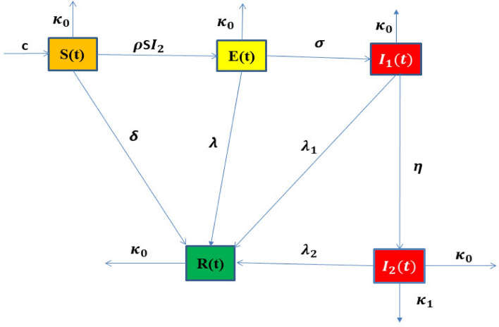
We provide a fractal-fractional adaptation of the time-delayed Hepatitis B model with optimal control. Over all population N(t) is distributed in five different groups:

• S(t): Refers to responsive patients, those who exhibit improvement or a change in their condition in response to a particular treatment, intervention, or stimulation. Generally speaking, “responsive patients” are individuals whose conditions or behavior change in response to specific inputs or variables in the model.

• E(t): Refers to exposed patients, those who have come into contact with a specific factor or condition of interest in a study or analysis without showing symptoms. Asymptomatic E(t) represents individuals who have been made aware of a particular disease, course of therapy, or other elements that the model is designed to examine for early detection. The term “exposed” indicates those who are subject to a specific situation or condition within the model; it does not inherently carry a negative connotation.

• $I_1(t)$: Refers to acutely contaminated individuals. This term usually describes people who have been exposed to a high concentration or dose of a contaminant in a short period. Acutely contaminated individuals may suffer from immediate health impacts or symptoms as a result of their exposure. It can be controlled by taking chemotherapy treatment.

• $I_2(t)$: Refers to persistently contaminated individuals, those who have been exposed to and maintain a certain level of contamination for a prolonged period. People exposed to and retaining a specific degree of contamination over an extended period are considered persistently polluted. This represents the chronic stage, which may cause liver infection, but with early detection and treatment, chronic stage infection can be reduced.

• R(t): Represents healed or recovered individuals. The term “recovered” implies that these individuals have completed the process of recuperation and are no longer affected by the condition under consideration. Individuals recover from both acute and chronic stages due to control measures like early detection and chemotherapy.

The transition of people from the class S to the class R is associated with the time delay of $\xi \ge 0$. The flow chart of the newly developed model $SE{I}_1{I}_{2}R$ is illustrated in Fig. 1.

Fig. 1.

Flow chart of the new developed model $SE{I}_1{I}_{2}R$.

In the Atangana-Baleanu sense, the new fractional order model can be formulated using the following non-linear fractional differential equations under the fractal-fractional operator:

$$\begin{array}{c}\hfill \left\{\begin{array}{cc}& DS(t)=c-\rho S(t)I_2(t)-({\kappa }_0+\delta )S(t),\hfill \\ \hfill & DE(t)=\rho S(t)I_2(t)-({\kappa }_0+\sigma +\lambda )E(t),\hfill \\ \hfill & D{I}_1(t)=\sigma E(t)-({\kappa }_0+\eta +{\lambda }_1)I_1(t),\hfill \\ \hfill & D{I}_2(t)=\eta I_1(t)-({\kappa }_0+{\kappa }_1+{\lambda }_2)I_2(t),\hfill \\ \hfill & DR(t)={\lambda }_1{I}_1(t)+{\lambda }_2{I}_2(t)+\delta S(t)-{\kappa }_{0}R(t)+\lambda E(t).\hfill \end{array}\right)\end{array}$$ 1

With the initial conditions

$$\begin{array}{c}\hfill S(0)=S^0\ge 0,E(0)=E^O\ge 0,I_1(0)=I_1^0\ge 0,I_2(0)=I_2^0\ge 0,R(0)=R^0\ge 0.\end{array}$$

The parameters of the system of given equations (model) (1) are listed as follows: c denotes the birth rate related to susceptible individuals, $\rho$ represents the rate of transfer involving asymptomatic patients, and ${\lambda }_1$ and ${\lambda }_2$ illustrate the recovery rates from infections at the acute or chronic stage due to asymptomatic measures for early detection process respectively. $\eta$ represents the rate at which acutely infected individuals become chronically infected, a dangerous stage of infection due to HBV and causes liver cirrhosis infection. ${\kappa }_0$ represents the natural death rate, with or without infection. ${\kappa }_1$ displays the mortality rate due to Hepatitis after causing liver cirrhosis, and $\delta$ illustrates the rate at which individuals recover due to a strong immune system, directly without spreading the infection and without medication, which is possible only due to early detection. Numerous studies have demonstrated that fractional-order systems outperform integer-order models in accurately representing the real world³⁷.

Now, we provide some fundamental concepts about differential equations acknowledged from³⁸, which will be utilized for our developed model.

Definitions: Let $0\le \mu$ , $\vartheta \le 1$, then U(t) in the Riemann-Liouville for fractal fractional operator with generalized Mittag-Leffler kernel is defined as:

$$\begin{array}{c}\hfill _{}^{\mathit{FFM}}{D}_{0,t}^{\mu ,\vartheta }(U(t))=\frac{AB(\mu )}{1-\mu }\frac{d}{d{t}^{\vartheta }}{\int }_0^t{E}_{\mu }\left[-,\frac{\mu }{1-\mu },{(t-\mathrm{\Omega })}^{\mu },U,(\mathrm{\Omega })\right]d\mathrm{\Omega },\end{array}$$

where $0<\mu ,\vartheta \le 1$ and $AB(\mu )=1-\mu +\frac{\mu }{\mathrm{\Gamma }(\mu )}.$

Thus, U(t) with order $(\mu ,\vartheta )$ and having Mittag-Leffler type kernel is defined as:

$$\begin{array}{c}\hfill _{}^{\mathit{FFM}}{D}_{0,t}^{\mu ,\vartheta }(U(t))=\frac{\vartheta (1-\mu )t^{\vartheta -1}U(t)}{AB(\mu )}+\frac{\mu \vartheta }{AB(\mu )}{\int }_0^t{\mathrm{\Omega }}^{\mu -1}(t-\mathrm{\Omega })U(\mathrm{\Omega })d\mathrm{\Omega }.\end{array}$$

Therefore, in accordance with model (1), we generate the on going fractional-order model using the fractal fractional derivative and the definitions given above:

$$\begin{array}{c}\hfill \left\{\begin{array}{cc}& _0^{\mathit{FFM}}{D}_t^{\varphi ,\phi }S(t)=c-\rho S(t)I_2(t)-({\kappa }_0+\delta )S(t),\hfill \\ \hfill & _0^{\mathit{FFM}}{D}_t^{\varphi ,\phi }E(t)=\rho S(t)I_2(t)-({\kappa }_0+\sigma +\lambda )E(t),\hfill \\ \hfill & _0^{\mathit{FFM}}{D}_t^{\varphi ,\phi }{I}_1(t)=\sigma E(t)-({\kappa }_0+\eta +{\lambda }_1)I_1(t),\hfill \\ \hfill & _0^{\mathit{FFM}}{D}_t^{\varphi ,\phi }{I}_2(t)=\eta I_1(t)-({\kappa }_0+{\kappa }_1+{\lambda }_2)I_2(t),\hfill \\ \hfill & _0^{\mathit{FFM}}{D}_t^{\varphi ,\phi }R(t)={\lambda }_1{I}_1(t)+{\lambda }_2{I}_2(t)+\delta S(t)-{\kappa }_{0}R(t)+\lambda E(t),\hfill \end{array}\right)\end{array}$$ 2

With the initial conditions:

$$\begin{array}{c}\hfill S(0)=S^0\ge 0,E(0)=E^O\ge 0,I_1(0)=I_1^0\ge 0,I_2(0)=I_2^0\ge 0,R(0)=R^0\ge 0.\end{array}$$

Quantitative analysis for the developed model

To demonstrate the suitability and limitations of the model, we are undertaking a procedure that ensures its validity, assuming it addresses universally significant problems with relevant parameter values. As outlined below

$$\begin{array}{cc}\hfill I_1(t)\ge & I_1^0{e}^{-({\kappa }_0+\eta +{\lambda }_1)t}\forall t\ge \xi ,\hfill \end{array}$$ 3

$$\begin{array}{cc}\hfill I_2(t)\ge & I_2^0{e}^{-({\kappa }_0+{\kappa }_1+{\lambda }_2)t}\forall t\ge \xi ,\hfill \end{array}$$ 4

$$\begin{array}{cc}\hfill R(t)\ge & R^0{e}^{(-{\kappa }_0)t}\forall t\ge \xi .\hfill \end{array}$$ 5

Defining the norm as:

$$\begin{array}{c}\hfill \Vert \mathcal{A}{\Vert }_{\infty }=\underset{t\in D_{\mathcal{A}}}{sup}\mid \mathcal{A}(t)\mid .\end{array}$$ 6

The domain of $\mathcal{A}$ is given as $D_{\mathcal{A}}$. For the class S(t), the norm is given as bellow:

$$\begin{array}{cc}\hfill S(t)=& c-\rho S{I}_2-({\kappa }_0+\delta )S,\hfill \\ \hfill \ge & -\rho S{I}_2-({\kappa }_0+\delta )S,\hfill \\ \hfill \ge & \left(-,\rho ,\mid ,I_2,\mid ,-,({\kappa }_0+\delta )\right)S,\hfill \\ \hfill \ge & \left(-,\rho ,\underset{t\in D_{I_2}}{sup},\mid ,I_2,\mid ,-,({\kappa }_0+\delta )\right)S,\hfill \\ \hfill \ge & \left(-,\rho ,\Vert ,I_2,{\Vert }_{\infty },-,({\kappa }_0+\delta )\right)S.\hfill \end{array}$$ 7

For ordinary derivative, we have.

$$\begin{array}{c}\hfill S(t)\ge S^0{e}^{(-\rho \Vert I_2{\Vert }_{\infty }-({\kappa }_0+\delta ))t}\forall t\ge \xi .\end{array}$$ 8

Now for the class E(t),

$$\begin{array}{cc}\hfill E(t)=& \rho S{I}_2-({\kappa }_0+\sigma +\lambda )E,\hfill \\ \hfill \ge & \rho \mid S{I}_2\mid -({\kappa }_0+\sigma +\lambda )E,\hfill \\ \hfill \ge & \rho \underset{t\in D_{S{I}_2}}{sup}\mid S{I}_2\mid -({\kappa }_0+\sigma +\lambda )E,\hfill \\ \hfill \ge & \rho \Vert S{I}_2{\Vert }_{\infty }-({\kappa }_0+\sigma +\lambda )E.\hfill \end{array}$$ 9

For ordinary derivative, we have

$$\begin{array}{c}\hfill E(t)\ge E^0{e}^{\rho \Vert S{I}_2{\Vert }_{\infty }-({\kappa }_0+\sigma +\lambda )E}\forall t\ge \xi .\end{array}$$ 10

The positive results with non-local operator are described below.

Boundedness and positiveness

Here, we illustrate the boundedness and positivity of the newly developed model.

Theorem 1

Let the initial conditions be

$$\begin{array}{c}\hfill \{S(0),E(0),I_1(0),I_2(0),R(0)\}\subset \mathrm{{\rm Y}},\end{array}$$

Then, if the solutions $S,E,I_1,I_2,R$ exist, they are all positive for all $t\ge 0$, and $\mathrm{{\rm Y}}$ is a space in $R_{+}^5$.

Proof

To demonstrate the positiveness of the solutions, we begin with an analysis using the method described in^39–41, which address real-world issues where values are inherently positive. We define the norm as given in Eq. (6):

$$\begin{array}{cc}\hfill _0^{\mathit{FFM}}{D}_t^{\varphi ,\phi }S(t)=& c-\rho I_2(t)-({\kappa }_0+\delta )),\forall t\ge 0\hfill \\ \hfill \ge & -(\rho I_2(t)+{\kappa }_0+\delta ),\forall t\ge 0\hfill \\ \hfill \ge & -(\rho \mid I_2(t)\mid +{\kappa }_0+\delta )S(t),\forall t\ge 0\hfill \\ \hfill \ge & -({\rho }_{t\in D_{\rho }}^{\mathit{sup}}\mid I_2(t)\mid +{\kappa }_0+\delta )S(t),\forall t\ge 0\hfill \\ \hfill \ge & -(\rho \Vert I_2{\Vert }_{\infty }+{\kappa }_0+\delta )S(t),\forall t\ge 0.\hfill \end{array}$$ 11

Using the definition of FFM and after simplification, we get

$$\begin{array}{c}\hfill S(t)\ge S(0)E_{\varphi }\left[-,\frac{d^{1-\phi }\varphi ({\kappa }_0+\delta +\rho \Vert I_2{\Vert }_{\infty })t^{\varphi }}{AB(\varphi )-(1-\varphi )({\kappa }_0+\delta +\rho \Vert I_2{\Vert }_{\infty })}\right],\forall t\ge 0.\end{array}$$ 12

Here, d is the time element. This indicates that $S(t)>0$ for all $t\ge 0$. Similarly, for the E(t), we have

$$\begin{array}{cc}\hfill _0^{\mathit{FFM}}{D}_t^{\varphi ,\phi }E(t)=& \rho S(t)I_2(t)-({\kappa }_0+\sigma +\lambda )E(t)\hfill \\ \hfill \ge & -({\kappa }_0+\sigma +\lambda )E,\forall t\ge 0,\hfill \end{array}$$

yielding

$$\begin{array}{c}\hfill E(t)\ge E(0)E_{\varphi }\left[-,\frac{d^{1-\phi }\varphi ({\kappa }_0+\sigma +\lambda )t^{\varphi }}{AB(\varphi )-(1-\varphi )({\kappa }_0+\sigma +\lambda )}\right],\forall t\ge 0.\end{array}$$ 13

Here, d is the time element. This indicates that $E(t)>0$ for all $t\ge 0$. For $I_1(t)$, we have

$$\begin{array}{cc}\hfill _0^{\mathit{FFM}}{D}_t^{\varphi ,\phi }{I}_1(t)=& \sigma E(t)-({\kappa }_0+\eta +{\lambda }_1)I_1(t),\forall t\ge 0\hfill \\ \hfill \ge & -({\kappa }_0+\eta +{\lambda }_1)I_1(t),\forall t\ge 0,\hfill \end{array}$$ 14

And this yields:

$$\begin{array}{c}\hfill I_1(t)\ge I_1(0)E_{\varphi }\left[-,\frac{d^{1-\phi }\varphi ({\kappa }_0+\eta +{\lambda }_1)t^{\varphi }}{AB(\varphi )-(1-\varphi )({\kappa }_0+\eta +{\lambda }_1)}\right],\forall t\ge 0.\end{array}$$ 15

Here, d is the time element. This indicates that $I_1(t)>0$ for all $t\ge 0$. For $I_2(t)$, we have

$$\begin{array}{cc}\hfill _0^{\mathit{FFM}}{D}_t^{\varphi ,\phi }{I}_2(t)=& \eta I_1(t)-({\kappa }_0+{\kappa }_1+{\lambda }_1)I_2(t),\forall t\ge 0\hfill \\ \hfill \ge & -({\kappa }_0+{\kappa }_1+{\lambda }_2)I_2(t),\forall t\ge 0,\hfill \end{array}$$

Yielding:

$$\begin{array}{c}\hfill I_2(t)\ge I_2(0)E_{\varphi }\left[-,\frac{d^{1-\phi }\varphi ({\kappa }_0+{\kappa }_1+{\lambda }_2)t^{\varphi }}{AB(\varphi )-(1-\varphi )({\kappa }_0+{\kappa }_1+{\lambda }_2)}\right],\forall t\ge 0.\end{array}$$ 16

Here, d is the time element. This indicates that $I_2(t)>0$ for all $t\ge 0$. For R(t), we have

$$\begin{array}{cc}\hfill _0^{\mathit{FFM}}{D}_t^{\varphi ,\phi }R(t)=& {\lambda }_1{I}_1(t)+{\lambda }_2{I}_2(t)+\delta S(t)-{\kappa }_{0}R(t)+\lambda E(t),\forall t\ge 0\hfill \\ \hfill \ge & -{\kappa }_{0}R(t),\forall t\ge 0,\hfill \end{array}$$ 17

yielding

$$\begin{array}{c}\hfill R(t)\ge R(0)E_{\varphi }\left[-,\frac{d^{1-\phi }\varphi ({\kappa }_0)t^{\varphi }}{AB(\varphi )-(1-\varphi )({\kappa }_0)}\right],\forall t\ge 0.\end{array}$$ 18

Here, d is the time element. This indicates that $R(t)>0$ for all $t\ge 0$. which shows that the developed system under the created hypothesis provides positive and bounded solutions for the HBV mathematical model. $\square$

Positive solutions with non-local operator

If each initial condition given is true for non-local operators, every outcome of (2) will be positive⁴².

• For Fractal-Fractional operator having a power law kernel, we obtain $\forall t\ge \xi$

  $$\begin{array}{c}\hfill \left\{\begin{array}{cc}& S(t)\ge S^0{F}_{\varphi }\left(-,{\omega }^{1-\phi },(-\rho \Vert I_2{\Vert }_{\infty }-({\kappa }_0+\delta )),t^{\varphi }\right),\hfill \\ \hfill & E(t)\ge E^0{F}_{\varphi }\left(\rho ,\Vert ,S,I_2,{\Vert }_{\infty },-,({\kappa }_0+\sigma +\lambda )\right),\hfill \\ \hfill & I_1(t)\ge I_1^0{F}_{\varphi }\left(-,{\omega }^{1-\phi },({\kappa }_0+\eta +{\lambda }_1),t^{\varphi }\right),\hfill \\ \hfill & I_2(t)\ge I_2^0{F}_{\varphi }\left(-,{\omega }^{1-\phi },({\kappa }_0+{\kappa }_1+{\lambda }_2)\right),\hfill \\ \hfill & R(t)\ge R^0{F}_{\varphi }\left(-,{\omega }^{1-\phi },(-{\kappa }_0),t^{\varphi }\right).\hfill \end{array}\right)\end{array}$$ 19

  Where $\omega$ is the time element.
• For Fractal-Fractional operator having an exponential kernel, we obtain $\forall t\ge \xi$.

  $$\begin{array}{c}\hfill \left\{\begin{array}{cc}& S(t)\ge S^{0}exp\left(-,\frac{{\chi }^{1-\phi }\varphi \left(-,\rho ,\Vert ,I_2,{\Vert }_{\infty },-,({\kappa }_0+\delta )\right)t}{\mu (\varphi )-(1-\varphi )\left[-,\rho ,\Vert ,I_2,{\Vert }_{\infty },-,({\kappa }_0+\delta )\right]}\right),\hfill \\ \hfill & E(t)\ge E^{0}exp\left(-,\frac{{\chi }^{1-\phi }\varphi (\rho \Vert S{I}_2{\Vert }_{\infty }-({\kappa }_0+\sigma +\lambda ))t}{\mu (\varphi )-(1-\varphi )\left[\rho ,\Vert ,S,I_2,{\Vert }_{\infty },-,({\kappa }_0+\sigma +\lambda )\right]}\right),\hfill \\ \hfill & I_1(t)\ge I_1^{0}exp\left(-,\frac{{\chi }^{1-\phi }\varphi ({\kappa }_0+\eta +{\lambda }_1)t}{\mu (\varphi )-(1-\varphi )\left[{\kappa }_0,+,\eta ,+,{\lambda }_1\right]}\right),\hfill \\ \hfill & I_2(t)\ge I_2^{0}exp\left(-,\frac{{\chi }^{1-\phi }\varphi ({\kappa }_0+{\kappa }_1+{\lambda }_2)t}{\mu (\varphi )-(1-\varphi )\left[{\kappa }_0,+,{\kappa }_1,+,{\lambda }_2\right]}\right),\hfill \\ \hfill & R(t)\ge R^{0}exp\left(-,\frac{{\chi }^{1-\phi }\varphi ({\kappa }_0)t}{\mu (\varphi )-(1-\varphi )\left[{\kappa }_0\right]}\right).\hfill \end{array}\right)\end{array}$$ 20
• For Fractal-Fractional operator having Mittag-leffler kernel, we obtain $\forall t\ge \xi$.

  $$\begin{array}{c}\hfill \left\{\begin{array}{cc}& S(t)\ge S^0{F}_{\varphi }\left(-,\frac{{\chi }^{1-\phi }\varphi \left(-,\rho ,\Vert ,I_2,{\Vert }_{\infty },-,({\kappa }_0+\delta )\right)t^{\varphi }}{\mu (\varphi )-(1-\varphi )\left[-,\rho ,\Vert ,I_2,{\Vert }_{\infty },-,({\kappa }_0+\delta )\right]}\right),\hfill \\ \hfill & E(t)\ge E^0{F}_{\varphi }\left(-,\frac{{\chi }^{1-\phi }\varphi (\rho \Vert S{I}_2{\Vert }_{\infty }-({\kappa }_0+\sigma +\lambda ))t^{\varphi }}{AB(\varphi )-(1-\varphi )\left[\rho ,\Vert ,S,I_2,{\Vert }_{\infty },-,({\kappa }_0+\sigma +\lambda )\right]}\right),\hfill \\ \hfill & I_1(t)\ge I_1^0{F}_{\varphi }\left(-,\frac{{\chi }^{1-\phi }\varphi ({\kappa }_0+\eta +{\lambda }_1)t^{\varphi }}{AB(\varphi )-(1-\varphi )\left[{\kappa }_0,+,\eta ,+,{\lambda }_1\right]}\right),\hfill \\ \hfill & I_2(t)\ge I_2^0{F}_{\varphi }\left(-,\frac{{\chi }^{1-\phi }\varphi ({\kappa }_0+{\kappa }_1+{\lambda }_2)t^{\varphi }}{AB(\varphi )-(1-\varphi )\left[{\kappa }_0,+,{\kappa }_1,+,{\lambda }_2\right]}\right),\hfill \\ \hfill & R(t)\ge R^0{F}_{\varphi }\left(-,\frac{{\chi }^{1-\phi }\varphi ({\kappa }_0)t^{\varphi }}{AB(\varphi )-(1-\varphi )\left[{\kappa }_0\right]}\right).\hfill \end{array}\right)\end{array}$$ 21

The above results show that the developed model provides positive solutions for utilizing different kernels under bounded domains for all t.

Positively invariant region

Lemma 1

If

$$\begin{array}{c}\hfill \daleth =\left\{(S,E,I_1,I_2,R),\in ,R_{+}^5,:,0,\le ,N,(t),\le ,\frac{c}{{\kappa }_0}\right\}.\end{array}$$ 22

When applied to non-negative starting circumstances, the region $\daleth$ is positively invariant and attracts all solutions of the proposed system in $R_{+}^5$ if $N(0)\le \frac{c}{{\kappa }_0}$.

Proof

We will show the positive solution to the model given in (2), and the results are outlined below:

$$\begin{array}{c}\hfill \left\{\begin{array}{cc}& _0^{\mathit{FFM}}{D}_t^{\varphi ,\phi }S(t){\mid }_{S=0}\ge c\ge 0,\hfill \\ \hfill & _0^{\mathit{FFM}}{D}_t^{\varphi ,\phi }E(t){\mid }_{E=0}\ge \rho S(t)I_2(t)\ge 0,\hfill \\ \hfill & _0^{\mathit{FFM}}{D}_t^{\varphi ,\phi }{I}_1(t){\mid }_{I_1=0}\ge \sigma E(t)\ge 0,\hfill \\ \hfill & _0^{\mathit{FFM}}{D}_t^{\varphi ,\phi }{I}_2(t){\mid }_{I_2=0}\ge \eta I_1(t)\ge 0,\hfill \\ \hfill & _0^{\mathit{FFM}}{D}_t^{\varphi ,\phi }R(t){\mid }_{R=0}\ge {\lambda }_1{I}_1(t)+{\lambda }_2{I}_2(t)+\delta S(t)+\lambda E(t)\ge 0.\hfill \end{array}\right)\end{array}$$ 23

The system (23) indicates that the vector field lies within $R_{+}^5$ on each hyperspace covering the non-negative orthant with $t\ge 0$. With the addition of the constituent elements of the human population in the model given by Eq. (2), we arrive at the following total population:

$$\begin{array}{cc}\hfill _0^{\mathit{FFM}}{D}_t^{\varphi ,\phi }N(t)=& _0^{\mathit{FFM}}{D}_t^{\varphi ,\phi }S(t){+}_0^{\mathit{FFM}}{D}_t^{\varphi ,\phi }E(t){+}_0^{\mathit{FFM}}{D}_t^{\varphi ,\phi }{I}_1(t){+}_0^{\mathit{FFM}}{D}_t^{\varphi ,\phi }{I}_2(t){+}_0^{\mathit{FFM}}{D}_t^{\varphi ,\phi }R(t),\hfill \\ \hfill =& c-{\kappa }_0(S(t)+E(t)+I_1(t)+I_2(t)+R(t)-{\kappa }_1{I}_1(t)).\hfill \end{array}$$

We can write

$$\begin{array}{c}\hfill _0^{\mathit{FFM}}{D}_t^{\varphi ,\phi }N(t)\le c-{\kappa }_{0}N.\end{array}$$ 24

Assuming $N(0)\le \frac{c}{{\kappa }_0}.$

$$\begin{array}{c}\hfill ⟹N(t)\le \frac{c}{{\kappa }_0}.\end{array}$$

Therefore, a solution of the fractional order model given in (2) persists in $\mathrm{\Gamma }$ for each $t>-\xi$. For the fractional model, this means that the closed set $\mathrm{\Gamma }$ is positively stable. Consequently, we are able to explore our fractional order model given in (2) within the feasible region.

$$\begin{array}{c}\hfill \daleth =\left\{(S,E,I_1,I_2,R),\in ,R_{+}^5,:,S,+,E,+,I_1,+,I_2,+,R,\le ,\frac{c}{{\kappa }_0}\right\}.\end{array}$$

$\square$

Qualitative analysis for the developed model

Constant functions reflect the states of an equilibrium system of equations that are differential with consistent coefficients. The balance in our circumstances is represented by:

$$\begin{array}{cc}\hfill _0^{\mathit{FFM}}{D}_t^{\varphi ,\phi }N(t)=& _0^{\mathit{FFM}}{D}_t^{\varphi ,\phi }S(t){=}_0^{\mathit{FFM}}{D}_t^{\varphi ,\phi }E(t){=}_0^{\mathit{FFM}}{D}_t^{\varphi ,\phi }{I}_1(t){=}_0^{\mathit{FFM}}{D}_t^{\varphi ,\phi }{I}_2(t){=}_0^{\mathit{FFM}}{D}_t^{\varphi ,\phi }R(t)=0.\hfill \end{array}$$

$\Rightarrow$;

$$\begin{array}{c}\hfill c-\rho S(t)I_2(t)-({\kappa }_0+\delta )S(t)=0,\\ \hfill \rho S(t)I_2(t)-({\kappa }_0+\sigma +\lambda )E(t)=0,\\ \hfill \sigma E(t)-({\kappa }_0+\eta +{\lambda }_1)I_1(t)=0,\\ \hfill \eta I_1(t)-({\kappa }_0+{\kappa }_1+{\lambda }_2)I_2(t)=0,\\ \hfill {\lambda }_1{I}_1(t)+{\lambda }_2{I}_2(t)+\delta S(t)-{\kappa }_{0}R(t)+\lambda E(t)=0.\end{array}$$

We end up with constant functions as a result. As a result, time delays have no impact on how equilibria present themselves. With constant parameters, the equilibria of hepatitis b models are therefore equivalent⁴³. We have the disease-free equilibrium states $E_0$ as:

$$\begin{array}{c}\hfill E_0=(S^0,E^0,I_1^0,I_2^0,R^0)=\left(S^0,=,\frac{c}{{\kappa }_0+\delta },,,0,,,0,,,0,,,R^0,=,\frac{c\delta }{({\kappa }_0+\delta ){\kappa }_0}\right).\end{array}$$ 25

There is an endemic equilibrium when there is an infection. By putting the right side of system given by Eq. (2) equal to 0 to reach the values of the endemic equilibrium $E_{}^{\ast }=(S_{}^{\ast },E_{}^{\ast },I_1^{\ast },I_2^{\ast },R_{}^{\ast })$ as given.

$$\begin{array}{c}\hfill S(t)\to 6.57067,E(t)\to 1.11667,I_1(t)\to 0.119643,I_2(t)\to 0.217532,R(t)\to 5.1638.\end{array}$$ 26

Reproductive Number

In order to get reproductive number $R_0$ we are having the next generation matrix procedure as used in⁴⁴ on model (2),

let us suppose:

$$\begin{array}{c}\hfill J_0=F-V.\end{array}$$

Construction of F and V is based on Next generation method in which infection rate may be taken in F and rest of the parameters must be in V, where F and V are as follows:

$$\begin{array}{cc}\hfill F=& \left[\begin{array}{ccccc}0& 0& 0& 0& 0\\ 0& -\sigma & 0& 0& 0\\ 0& \sigma & 0& 0& 0\\ 0& 0& \eta & 0& 0\\ 0& 0& 0& 0& 0\\ \end{array}\right]\hfill \\ \hfill V=& \left[\begin{array}{ccccc}{\kappa }_0+\delta & 0& 0& \frac{\rho c}{{\kappa }_0+\delta }& 0\\ 0& {\kappa }_0+\lambda & 0& -\frac{\rho c}{{\kappa }_0+\delta }& 0\\ 0& 0& {\kappa }_0+\eta +{\lambda }_1& 0& 0\\ 0& 0& 0& {\kappa }_0+{\kappa }_1+{\lambda }_2& 0\\ -\delta & -\lambda & -{\lambda }_1& -{\lambda }_2& {\kappa }_0\\ \end{array}\right].\hfill \end{array}$$

Now using

$$\begin{array}{c}\hfill K=F{V}^{-1},\end{array}$$ 27

Also using the characteristics equation $det(K-\mathrm{\Lambda }I)=0$, We obtained $\mathrm{\Lambda }$ by solving characteristics equations which shows the reproductive number $R_0$. We find the reproductive number using the next generation technique and get the following:

$$\begin{array}{c}\hfill R_0=\frac{c\rho \sigma \eta }{({\kappa }_0+\delta )+({\kappa }_0+{\kappa }_1+{\lambda }_2)+({\kappa }_0+{\lambda }_2+{\lambda }_1)+({\kappa }_0+\lambda +\sigma )},\end{array}$$ 28

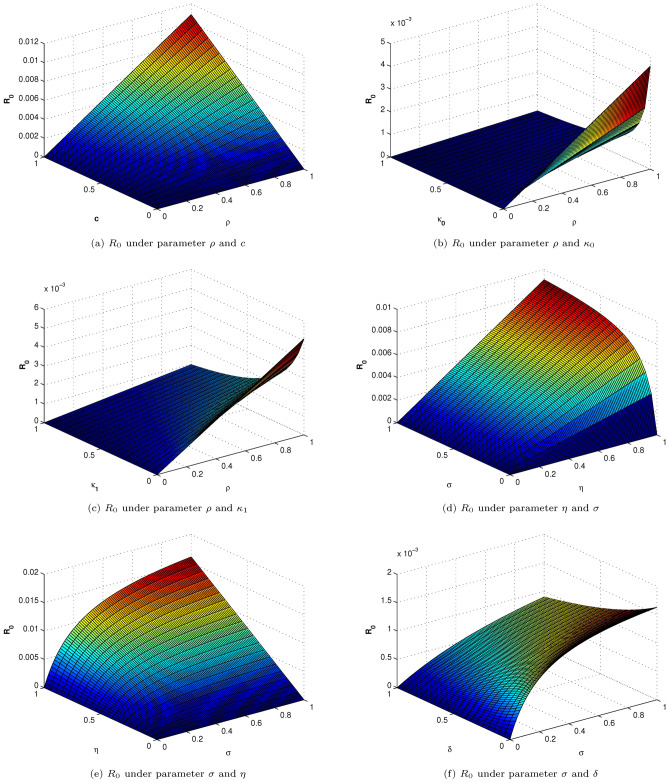
Which is less than one under the considered parameters, and it will rise if we rise up the rate of $\eta$, c and $\rho$.

Sensitivity Analysis

Sensitivity analysis is used to assess how different elements, when combined with uncertain data, affect a model’s stability. Also, the research can pinpoint the crucial variables. If we take into account the partial derivative of the threshold for the pertinent parameters, we can investigate the sensitivity of $R_0$.

Reproductive number is:

$$\begin{array}{cc}\hfill R_0=& \frac{c\rho \sigma \eta }{({\kappa }_0+\delta )+({\kappa }_0+{\kappa }_1+{\lambda }_2)+({\kappa }_0+{\lambda }_2+{\lambda }_1)+({\kappa }_0+\lambda +\sigma )},\hfill \\ \hfill \frac{\partial R_0}{\partial {\kappa }_0}=& \frac{1}{{({\kappa }_0+\delta )}^2{({\kappa }_0+{\kappa }_1+{\lambda }_2)}^2{({\kappa }_0+{\lambda }_2+{\lambda }_1)}^2{({\kappa }_0+\lambda +\sigma )}^2}\hfill \\ \hfill & \times [-(({\kappa }_0+\delta )({\kappa }_0+{\kappa }_1+{\lambda }_2)({\kappa }_0+{\lambda }_2+{\lambda }_1))-({\kappa }_0+\delta )({\kappa }_0+{\kappa }_1+{\lambda }_2)({\kappa }_0+\lambda +\sigma )\hfill \\ \hfill & -({\kappa }_0+\delta )({\kappa }_0+{\lambda }_2+{\lambda }_1)({\kappa }_0+\lambda +\sigma )-({\kappa }_0+{\kappa }_1+{\lambda }_2)({\kappa }_0+{\lambda }_2+{\lambda }_1)({\kappa }_0+\lambda +\sigma )]\eta <0,\hfill \\ \hfill \frac{\partial R_0}{\partial c}=& \frac{\rho \sigma \eta }{({\kappa }_0+\delta )({\kappa }_0+{\kappa }_1+{\lambda }_2)({\kappa }_0+{\lambda }_2+{\lambda }_1)({\kappa }_0+\lambda +\sigma )}>0,\hfill \\ \hfill \frac{\partial R_0}{\partial \rho }=& \frac{\rho \sigma \eta }{({\kappa }_0+\delta )({\kappa }_0+{\kappa }_1+{\lambda }_2)({\kappa }_0+{\lambda }_2+{\lambda }_1)({\kappa }_0+\lambda +\sigma )}>0\hfill \\ \hfill \frac{\partial R_0}{\partial \sigma }=& -\frac{c\rho ({\kappa }_0+\lambda )\eta }{({\kappa }_0+\delta )({\kappa }_0+{\kappa }_1+{\lambda }_2)({\kappa }_0+{\lambda }_2+{\lambda }_1){({\kappa }_0+\lambda +\sigma )}^2}>0,\hfill \\ \hfill \frac{\partial R_0}{\partial \eta }=& \frac{c\rho \sigma \eta }{({\kappa }_0+\delta )({\kappa }_0+{\kappa }_1+{\lambda }_2)({\kappa }_0+{\lambda }_2+{\lambda }_1)({\kappa }_0+\lambda +\sigma )}>0,\hfill \\ \hfill \frac{\partial R_0}{\partial \delta }=& -\frac{c\rho \sigma \eta }{{({\kappa }_0+\delta )}^2({\kappa }_0+{\kappa }_1+{\lambda }_2)({\kappa }_0+{\lambda }_2+{\lambda }_1)({\kappa }_0+\lambda +\sigma )}<0,\hfill \\ \hfill \frac{\partial R_0}{\partial {\kappa }_1}=& -\frac{c\rho \sigma \eta }{({\kappa }_0+\delta ){({\kappa }_0+{\kappa }_1+{\lambda }_2)}^2({\kappa }_0+{\lambda }_2+{\lambda }_1)({\kappa }_0+\lambda +\sigma )}<0,\hfill \\ \hfill \frac{\partial R_0}{\partial {\lambda }_2}=& -\frac{c\rho (2{\kappa }_0+{\kappa }_1+2{\lambda }_2+{\lambda }_1)\sigma \eta }{({\kappa }_0+\delta ){({\kappa }_0+{\kappa }_1+{\lambda }_2)}^2{({\kappa }_0+{\lambda }_2+{\lambda }_1)}^2({\kappa }_0+\lambda +\sigma )}<0,\hfill \\ \hfill \frac{\partial R_0}{\partial {\lambda }_1}=& -\frac{c\rho \sigma \eta }{({\kappa }_0+\delta )({\kappa }_0+{\kappa }_1+{\lambda }_2){({\kappa }_0+{\lambda }_2+{\lambda }_1)}^2({\kappa }_0+\lambda +\sigma )}<0,\hfill \\ \hfill \frac{\partial R_0}{\partial \lambda }=& -\frac{c\rho \sigma \eta }{({\kappa }_0+\delta )({\kappa }_0+{\kappa }_1+{\lambda }_2)({\kappa }_0+{\lambda }_2+{\lambda }_1){({\kappa }_0+\lambda +\sigma )}^2}<0.\hfill \end{array}$$ 29

It becomes clear that $R_0$ is incredibly sensitive as we alter the parameters. The parameters $\delta$, ${\kappa }_1$, $\lambda$, ${\lambda }_1$ and ${\lambda }_2$ are shrinking in this work whereas the variables c, $\rho$, $\sigma$ and $\eta$ are expanding. Figure 2 illustrates this reproductive number behavior under different parameters.

Fig. 2.

Reproductive number behavior under different parameters.

In order to confirm the bounded behavior of the newly developed Hepatitis B virus model, combinations of each compartment with the influence of the other compartments are examined. Here, it has extremely complicated effects on the populace; the hepatitis connection system is continuous and time-dependent. Upon determining the rate of change under various parameters, it is apparent that the value of $R_0$ is quite sensitive. Therefore, medication should follow prevention for effective infection control. As shown in Fig. 2, the indices previously mentioned assist in identifying the crucial factors that influence the infection’s potential to spread.

All of the aforementioned sub-figures demonstrate how the value of $R_0$ behaves in a very responsive manner. The behavior with respect to $\rho$ with $k_0$ and $k_1$, and the behavior of $\rho$ with c, $\eta$ with $\sigma$, and $\sigma$ with $\eta$ are similar with minor effects. It is also observed that $R_0$ is most sensitive under the rate of change of different parameters, as the rate of change of these parameters $\eta$ and $\sigma$ provides a high risk of disease spread. This needs to be maintained within a specific range; otherwise, chronic stage infection will rise and cause liver cirrhosis. However, all of the sub-figures show that each parameter’s rate of change is limited, which is crucial for stable conditions.

Locally and globally analysis of the model

Local stability analysis for equilibrium

As per equilibria, local stability is confirmed by the subsequent theorem.

Theorem 2

When $R_0$ is less than 1, the disease-free equilibrium point of the suggested fractional-order Hepatitis B Virus (HBV) model shows local asymptotic stability.

Proof

Assume that the suggested system is stable at $E_0$. The Jacobian matrix, which can be shortened to J, is as follows:

$$\begin{array}{c}\hfill J=\left[\begin{array}{ccccc}-\rho I_2-({\kappa }_0+\delta )& 0& 0& \rho S& 0\\ \rho I_2& -({\kappa }_0+\sigma +\lambda )& 0& \rho S& 0\\ 0& \sigma & -({\kappa }_0+\eta +{\lambda }_1)& 0& 0\\ 0& 0& \eta & -({\kappa }_0+{\kappa }_1+{\lambda }_2)& 0\\ \delta & \lambda & {\lambda }_1& {\lambda }_2& -{\kappa }_0\\ \end{array}\right]\end{array}$$

At $E_0$

$$\begin{array}{c}\hfill J_o=\left[\begin{array}{ccccc}-({\kappa }_0+\delta )& 0& 0& -\frac{\rho c}{{\kappa }_0+\delta }& 0\\ 0& -({\kappa }_0+\sigma +\lambda )& 0& \frac{\rho c}{{\kappa }_0+\delta }& 0\\ 0& \sigma & -({\kappa }_0+{\kappa }_1+{\lambda }_2)& 0& 0\\ 0& 0& \eta & -({\kappa }_0+{\kappa }_1+{\lambda }_2)& 0\\ \delta & \lambda & {\lambda }_1& {\lambda }_2& -{\kappa }_0\\ \end{array}\right]\end{array}$$

So, the characteristics equation is

$$\begin{array}{cc}\hfill \mid J_0-\mathrm{\Lambda }I\mid =& 0\hfill \\ \hfill \mid J_0-\mathrm{\Lambda }I\mid =& \left|\begin{array}{ccccc}-({\kappa }_0+\delta )-\mathrm{\Lambda }& 0& 0& -\frac{\rho c}{{\kappa }_0+\delta }& 0\\ 0& -({\kappa }_0+\sigma +\lambda )-\mathrm{\Lambda }& 0& \frac{\rho c}{{\kappa }_0+\delta }& 0\\ 0& \sigma & -({\kappa }_0+{\kappa }_1+{\lambda }_2)-\mathrm{\Lambda }& 0& 0\\ 0& 0& \eta & -({\kappa }_0+{\kappa }_1+{\lambda }_2)-\mathrm{\Lambda }& 0\\ \delta & \lambda & {\lambda }_1& {\lambda }_2& -{\kappa }_0-\mathrm{\Lambda }\\ \end{array}\right|=0\hfill \end{array}$$ 30

The eigenvalues $\mathrm{\Lambda }$ have been obtained from the above determinant. The calculated eigenvalues are as follows:

$$\begin{array}{cc}\hfill \mathrm{\Lambda }=& -0.05,\hfill \\ \hfill \mathrm{\Lambda }=& -0.03,\hfill \\ \hfill \mathrm{\Lambda }=& -0.215506+0.0137158i,\hfill \\ \hfill \mathrm{\Lambda }=& -0.00398878-1.04083\times {10}^{-17}i.\hfill \end{array}$$

In systems modeled by differential equations, negative real parts of eigenvalues suggests that perturbations or disturbances will decay over time, leading to stable behavior. The above results show that the real parts of all the eigenvalues are negative, indicating that the system is locally asymptotically stable for $R_0<1$. $\square$

Global Stability Analysis

Applying Lyapunov’s method and Lasalle’s invariance principle, the global stability analysis is shown to determine the prerequisites for epidemic extermination.

First derivative of Lyapunov

Theorem 3

As $R_0>1$, then endemic equilibrium points of the $SE{I}_1{I}_{2}R$ model is globally asynchronously stable

Proof

In order to proove this the Lyapunov function is going to be written as.

$$\begin{array}{cc}\hfill L(S_{}^{\ast },(E_{}^{\ast },I_1^{\ast },I_2^{\ast },R\ast )=& \left(S,,-,S_{}^{\ast },-,,S_{}^{\ast },log,\frac{S}{S_{}^{\ast }}\right)+(E-E_{}^{\ast }-E_{}^{\ast }log\frac{E}{E_{}^{\ast }})+\left(I_1,-,,I_1^{\ast },-,I_1^{\ast },log,\frac{I_1}{I_1^{\ast }}\right)\hfill \\ \hfill & +\left(I_2,-,I_2^{\ast },,-,I_2^{\ast },log,\frac{I_2}{I_2^{\ast }}\right)+\left(R,-,R_{}^{\ast },-,,R_{}^{\ast },log,\frac{R}{R_{}^{\ast }}\right).\hfill \end{array}$$

Taking derivative we have;

$$\begin{array}{cc}\hfill _0^{\mathit{FFM}}{D}_t^{\varphi ,\phi }L=& \left(\frac{S-S_{}^{\ast }}{S}\right)_0^{\mathit{FFM}}{D}_t^{\varphi ,\phi }S(t)+\left(\frac{E-E_{}^{\ast }}{E}\right)_0^{\mathit{FFM}}{D}_t^{\varphi ,\phi }E(t)+\left(\frac{I_1-I_1^{\ast }}{I_1}\right)_0^{\mathit{FFM}}{D}_t^{\varphi ,\phi }{I}_1(t)\hfill \\ \hfill & +\left(\frac{I_2-I_2^{\ast }}{I_2}\right)_0^{\mathit{FFM}}{D}_t^{\varphi ,\phi }{I}_2(t)+\left(\frac{R-R_{}^{\ast }}{R}\right)_0^{\mathit{FFM}}{D}_t^{\varphi ,\phi }R(t).\hfill \end{array}$$

We have

$$\begin{array}{cc}\hfill _0^{\mathit{FFM}}{D}_t^{\varphi ,\phi }L=& \left(\frac{S-S_{}^{\ast }}{S}\right)(c-\rho S{I}_2-({\kappa }_0+\delta )S)+\left(\frac{E-E_{}^{\ast }}{E}\right)(\rho S(t)I_2(t)-({\kappa }_0+\sigma +\gamma )E(t))\hfill \\ \hfill & +\left(\frac{I_1-I_1^{\ast }}{I_1}\right)(\sigma E-({\kappa }_0+\eta +{\lambda }_1)I_1)+\left(\frac{I_2-I_2^{\ast }}{I_2}\right)(\eta I_1-({\kappa }_0+{\kappa }_1+{\gamma }_2)I_2)\hfill \\ \hfill & +\left(\frac{R-R_{}^{\ast }}{R}\right)({\lambda }_1{I}_1+{\gamma }_2{I}_2+\delta S-{\kappa }_{0}R+\gamma E).\hfill \end{array}$$

By putting $S=S-S_{}^{\ast }$,$E=E-E_{}^{\ast }$,$I_1=I_1-I_1^{\ast }$, $I_2=I_2-I_2^{\ast }$, $R=R-R_{}^{\ast }$ leads to:

$$\begin{array}{cc}\hfill _0^{\mathit{FFM}}{D}_t^{\varphi ,\phi }L=& \left(\frac{S-S_{}^{\ast }}{S}\right)(c-\rho (S-S_{}^{\ast })(I_2-I_2^{\ast })-({\kappa }_0+\delta )(S-S_{}^{\ast }))\hfill \\ \hfill & +(\frac{E-E_{}^{\ast }}{E})(\rho (S-S_{}^{\ast })((I_2-I_2^{\ast }))-({\kappa }_0+\sigma +\lambda )(E-E_{}^{\ast }))\hfill \\ \hfill & +\left(\frac{I_1-I_1^{\ast }}{I_1}\right)(\sigma (E-E_{}^{\ast }))-({\kappa }_0+\eta +{\lambda }_1)(I_1-I_1^{\ast })+\left(\frac{I_2-I_2^{\ast }}{I_2}\right)(\eta (I_1-I_1^{\ast })-({\kappa }_0+{\kappa }_1+{\lambda }_2(I_2-I_2^{\ast }))\hfill \\ \hfill & +(\frac{R-R_{}^{\ast }}{R})({\lambda }_1(I_1-I_1^{\ast })+{\lambda }_2(I_2-I_2^{\ast }))+\delta (S-S_{}^{\ast })-{\kappa }_0(R-R_{}^{\ast })+\sigma (E-E_{}^{\ast })).\hfill \\ \hfill _0^{\mathit{FFM}}{D}_t^{\varphi ,\phi }L=& c-c\frac{S_{}^{\ast }}{S}-\rho I_2\frac{(S-S_{}^{\ast })_{}^2}{S}+\rho I_2^{\ast }\frac{(S-S_{}^{\ast })_{}^2}{S}-({\kappa }_0+\delta )\frac{(S-S_{}^{\ast })_{}^2}{S}\hfill \\ \hfill & +\rho I_{2}S-\rho I_2^{\ast }S-\rho I_{2}S_{}^{\ast }+\rho I_2^{\ast }S_{}^{\ast }-I_{2}S\rho \frac{E_{}^{\ast }}{E}+\rho SI_2^{\ast }\frac{E_{}^{\ast }}{E}\hfill \\ \hfill & +\rho S_{}^{\ast }{I}_2\frac{E_{}^{\ast }}{E}-S_{}^{\ast }\rho I_2^{\ast }\frac{E_{}^{\ast }}{E}-\rho I_1^{\ast }S_{}^{\ast }\frac{E_{}^{\ast }}{E}+\sigma E-\sigma E_{}^{\ast }-\sigma E\frac{I_1^{\ast }}{I_1}+\sigma E_{}^{\ast }\frac{I_1^{\ast }}{I_1}-({\kappa }_0+\eta +{\lambda }_1)\frac{(I_1-I_1^{\ast })_{}^2}{I_1}\hfill \\ \hfill & +\eta I_1-\eta I_1\frac{I_2^{\ast }}{I_2}-\eta I_1^{\ast }+\eta I_1^{\ast }\frac{I_2^{\ast }}{I_2}-({\kappa }_0+{\kappa }_1+{\lambda }_2)\frac{(I_2-I_2^{\ast })_{}^2}{I_2}+{\lambda }_1{I}_1-{\lambda }_{1}I_1^{\ast }-{\lambda }_1{I}_1\frac{R_{}^{\ast }}{R}+{\lambda }_{1}I_1^{\ast }\frac{R_{}^{\ast }}{R}+{\lambda }_2{I}_2\hfill \\ \hfill & -{\lambda }_{2}I_2^{\ast }-{\lambda }_2{I}_2\frac{R_{}^{\ast }}{R}+{\lambda }_{2}I_2^{\ast }\frac{R_{}^{\ast }}{R}+\delta S-\delta S_{}^{\ast }-\delta S\frac{R_{}^{\ast }}{R}+\delta S_{}^{\ast }\frac{R_{}^{\ast }}{R}\hfill \\ \hfill & -{\kappa }_0\frac{(R-R_{}^{\ast })_{}^2}{R}+\sigma E-\sigma E_{}^{\ast }-\sigma E\frac{R_{}^{\ast }}{R}+\sigma E_{}^{\ast }\frac{R_{}^{\ast }}{R}.\hfill \end{array}$$ 31

We can write

$$\begin{array}{c}\hfill _0^{\mathit{FFM}}{D}_t^{\varphi ,\phi }L=M-G.\end{array}$$ 32

Where

$$\begin{array}{cc}\hfill M=& c+\rho I_2^{\ast }\frac{(S-S_{}^{\ast })_{}^2}{S}+\rho I_{2}S+\rho I_2^{\ast }S_{}^{\ast }+\rho SI_2^{\ast }\frac{E_{}^{\ast }}{E}+\rho S_{}^{\ast }{I}_2\frac{E_{}^{\ast }}{E}+\sigma E+\sigma E_{}^{\ast }\frac{I_1^{\ast }}{I_1}\hfill \\ \hfill & +\eta I_1+\eta I_1^{\ast }\frac{I_2^{\ast }}{I_2}+{\lambda }_1{I}_1-{\lambda }_{1}I_1^{\ast }+{\lambda }_{1}I_1^{\ast }\frac{R_{}^{\ast }}{R}+{\lambda }_{2}I_2^{\ast }\frac{R_{}^{\ast }}{R}+\delta S+\delta S_{}^{\ast }\frac{R_{}^{\ast }}{R}+\sigma E+\sigma E_{}^{\ast }\frac{R_{}^{\ast }}{R}.\hfill \end{array}$$

And

$$\begin{array}{cc}\hfill G=& c\frac{S_{}^{\ast }}{S}+\rho I_2\frac{(S-S_{}^{\ast })_{}^2}{S}+({\kappa }_0+\delta )\frac{(S-S_{}^{\ast })_{}^2}{S}+\rho I_2^{\ast }S+\rho I_{2}S_{}^{\ast }+I_{2}S\rho \frac{E_{}^{\ast }}{E}\hfill \\ \hfill & +S_{}^{\ast }\rho I_2^{\ast }\frac{E_{}^{\ast }}{E}+\rho I_1^{\ast }S_{}^{\ast }\frac{E_{}^{\ast }}{E}+\sigma E_{}^{\ast }+\sigma E\frac{I_1^{\ast }}{I_1}+({\kappa }_0+\eta +{\lambda }_1)\frac{(I_1-I_1^{\ast })_{}^2}{I_1}\hfill \\ \hfill & +\eta I_1\frac{I_2^{\ast }}{I_2}+\eta I_1^{\ast }+({\kappa }_0+{\kappa }_1+{\lambda }_2)\frac{(I_2+I_2^{\ast })_{}^2}{I_2}+{\lambda }_{1}I_1^{\ast }+{\lambda }_1{I}_1\frac{R_{}^{\ast }}{R}\hfill \\ \hfill & +{\lambda }_{2}I_2^{\ast }+{\lambda }_2{I}_2\frac{R_{}^{\ast }}{R}+\delta S_{}^{\ast }+\delta S\frac{R_{}^{\ast }}{R}+{\kappa }_0\frac{(R-R_{}^{\ast })_{}^2}{R}+\sigma E_{}^{\ast }+\sigma E\frac{R_{}^{\ast }}{R}.\hfill \end{array}$$ 33

We conclude that if $M<G$ this yields $\frac{\mathit{dL}}{\mathit{dt}}<0$ as long as;

$$\begin{array}{cc}\hfill S=& S_{}^{\ast },E=E_{}^{\ast },I_1=I_1^{\ast },I_2=I_2^{\ast },R=R_{}^{\ast }.\hfill \\ \hfill 0=& M-G\Rightarrow \frac{\mathit{dL}}{\mathit{dt}}=0.\hfill \end{array}$$ 34

From the above calculation, we obtain that

$$\begin{array}{c}\hfill (S_{}^{\ast },E_{}^{\ast },I_1^{\ast },I_2^{\ast },R_{}^{\ast })\in \mathrm{\Gamma }:\frac{\mathit{dL}}{\mathit{dt}}=0.\end{array}$$ 35

Here is the point $E_{}^{\ast }$, the endemic equilibrium of the newly developed model. Using LaSalle’s invariance principle, $E_{}^{\ast }$ is globally asymptotically stable in $\mathrm{\Gamma }$ if $G<M$. $\square$

Existence and uniqueness analysis

In the context of a Banach space, fixed point mappings offer a comprehensive approach to studying the existence of a unique solution. A fixed point mapping theorem indicates that at least one solution exists for the suggested system described by Equ. (2) within the interval $[0,\mathcal{T}]$⁴⁵. Consider the system defined by Eq. (2) as:

$$\begin{array}{c}\hfill \left\{\begin{array}{cc}& _0^{\mathit{FFM}}{D}_t^{\varphi ,\phi }S(t)=c-\rho S(t)I_2(t)-({\kappa }_0+\delta )S(t)=\tilde{S}(t,S(t)),\hfill \\ \hfill & _0^{\mathit{FFM}}{D}_t^{\varphi ,\phi }E(t)=\rho S(t)I_2(t)-({\kappa }_0+\sigma +\lambda )E(t)=\tilde{E}(t,E(t)),\hfill \\ \hfill & _0^{\mathit{FFM}}{D}_t^{\varphi ,\phi }{I}_1(t)=\sigma E(t)-({\kappa }_0+\eta +{\lambda }_1)I_1(t)=\widetilde{I_1}(t,I_1(t)),\hfill \\ \hfill & _0^{\mathit{FFM}}{D}_t^{\varphi ,\phi }{I}_2(t)=\eta I_1(t)-({\kappa }_0+{\kappa }_1+{\lambda }_2)I_2(t))=\widetilde{I_2}(t,I_2(t)),\hfill \\ \hfill & _0^{\mathit{FFM}}{D}_t^{\varphi ,\phi }R(t)={\lambda }_1{I}_1(t)+{\lambda }_2{I}_2(t)+\delta S(t)-{\kappa }_{0}R(t)+\lambda E(t)=\tilde{R}(t,R(t)).\hfill \end{array}\right)\end{array}$$ 36

The modification of the system (36) can be represented as follows:

$$\begin{array}{c}\hfill \left\{\begin{array}{cc}& _0^{\mathit{FFM}}{D}_t^{\varphi ,\phi }S(t)=S^0(t)+\frac{\phi (1-\varphi )t^{\phi -1}}{AB(\varphi )}\tilde{S}(t,S(t))+\frac{\varphi \phi }{AB(\varphi )\mathrm{\Phi }(\varphi )}{\int }_0^t{(t-\xi )}^{\varphi -1}{\xi }^{\phi -1}\tilde{S}(\xi ,S(\xi ))d\xi =A_1+A_2,\hfill \\ \hfill & _0^{\mathit{FFM}}{D}_t^{\varphi ,\phi }E(t)=E^0(t)+\frac{\phi (1-\varphi )t^{\phi -1}}{AB(\varphi )}\tilde{E}(t,E(t))+\frac{\varphi \phi }{AB(\varphi )\mathrm{\Phi }(\varphi )}{\int }_0^t{(t-\xi )}^{\varphi -1}{\xi }^{\phi -1}\tilde{E}(\xi ,E(\xi ))d\xi =B_1+B_2,\hfill \\ \hfill & _0^{\mathit{FFM}}{D}_t^{\varphi ,\phi }{I}_1(t)=I_1^0(t)+\frac{\phi (1-\varphi )t^{\phi -1}}{AB(\varphi )}\widetilde{I_1}(t,I_1(t))+\frac{\varphi \phi }{AB(\varphi )\mathrm{\Phi }(\varphi )}{\int }_0^t{(t-\xi )}^{\varphi -1}{\xi }^{\phi -1}\widetilde{I_1}(\xi ,I_1(\xi ))d\xi =C_1+C_2,\hfill \\ \hfill & _0^{\mathit{FFM}}{D}_t^{\varphi ,\phi }{I}_2(t)=I_2^0(t)+\frac{\phi (1-\varphi )t^{\phi -1}}{AB(\varphi )}\widetilde{I_2}(t,I_2(t))+\frac{\varphi \phi }{AB(\varphi )\mathrm{\Phi }(\varphi )}{\int }_0^t{(t-\xi )}^{\varphi -1}{\xi }^{\phi -1}\widetilde{I_2}(\xi ,I_2(\xi ))d\xi =D_1+D_2,\hfill \\ \hfill & _0^{\mathit{FFM}}{D}_t^{\varphi ,\phi }R(t)=R^0(t)+\frac{\phi (1-\varphi )t^{\phi -1}}{AB(\varphi )}\tilde{R}(t,R(t))+\frac{\varphi \phi }{AB(\varphi )\mathrm{\Phi }(\varphi )}{\int }_0^t{(t-\xi )}^{\varphi -1}{\xi }^{\phi -1}\tilde{R}(\xi ,R(\xi ))d\xi =E_1+E_2,\hfill \end{array}\right)\end{array}$$ 37

Where

$$\begin{array}{c}\hfill \left\{\begin{array}{c}{A}_1=S^0(t)+\frac{\phi (1-\varphi )t^{\phi -1}}{AB(\varphi )}\tilde{S}(t,S(t)),A_2=\frac{\varphi \phi }{AB(\varphi )\mathrm{\Phi }(\varphi )}{\int }_0^t{(t-\xi )}^{\varphi -1}{\xi }^{\phi -1}\tilde{S}(\xi ,S(\xi ))d\xi ,\hfill \\ B_1=E^0(t)+\frac{\phi (1-\varphi )t^{\phi -1}}{AB(\varphi )}\tilde{E}(t,E(t)),B_2=\frac{\varphi \phi }{AB(\varphi )\mathrm{\Phi }(\varphi )}{\int }_0^t{(t-\xi )}^{\varphi -1}{\xi }^{\phi -1}\tilde{E}(\xi ,E(\xi ))d\xi ,\hfill \\ C_1=I_1^0(t)+\frac{\phi (1-\varphi )t^{\phi -1}}{AB(\varphi )}\widetilde{I_1}(t,I_1(t)),C_2=\frac{\varphi \phi }{AB(\varphi )\mathrm{\Phi }(\varphi )}{\int }_0^t{(t-\xi )}^{\varphi -1}{\xi }^{\phi -1}\widetilde{I_1}(\xi ,I_1(\xi ))d\xi ,\hfill \\ D_1=I_2^0(t)+\frac{\phi (1-\varphi )t^{\phi -1}}{AB(\varphi )}\widetilde{I_2}(t,I_2(t)),D_2\frac{\varphi \phi }{AB(\varphi )\mathrm{\Phi }(\varphi )}{\int }_0^t{(t-\xi )}^{\varphi -1}{\xi }^{\phi -1}\widetilde{I_2}(\xi ,I_2(\xi ))d\xi ,\hfill \\ E_1=R^0(t)+\frac{\phi (1-\varphi )t^{\phi -1}}{AB(\varphi )}\tilde{R}(t,R(t)),E_2=\frac{\varphi \phi }{AB(\varphi )\mathrm{\Phi }(\varphi )}{\int }_0^t{(t-\xi )}^{\varphi -1}{\xi }^{\phi -1}\tilde{R}(\xi ,R(\xi ))d\xi .\hfill \end{array}\right)\end{array}$$ 38

We establish the fundamental element of the regulating Eq. (36), where $P(A_1,B_1,C_1,D_1,E_1)$ are contraction maps and $U(A_2,B_2,C_2,D_2,E_2)$ as continuous compact integral parts using Krasnoselski’s fixed point theorem.

Theorem 4

The non-linear map $P(A_1,B_1,C_1,D_1,E_1)$: $[0,\mathbb{T}]\times \mathbb{R}\times \mathbb{R}\to {\mathbb{R}}^5$ given in (36) illustrates Lipschitz contractive condition for constants and $P(M_A,M_B,M_C,M_D,M_E>0).$

Proof

Assuming the operator $P(A_1,B_1,C_1,D_1,E_1)$: $[0,\mathbb{T}]\times \mathbb{R}\times \mathbb{R}\to {\mathbb{R}}^5$ is defined in a complete normed space.

$$\begin{array}{c}\hfill \Vert (S,E,I_1,I_2,R)\Vert =\underset{t\in [0,\mathbb{T}]}{max}\Vert S(t),E(t),I_1(t),I_2(t),R(t)\Vert ,S,E,I_1,I_2,Rt\in [0,\mathbb{T}].\end{array}$$ 39

(i): First of all, $P(A_1,B_1,C_1,D_1,E_1)$ is a contraction map. For S(t) and $\tilde{S}(t)$,

$$\begin{array}{cc}\hfill \Vert A(S,E,I_1,I_2,R)(t)-A(\tilde{S},E,I_1,I_2,R)(t)\Vert =& \Vert c-\rho S{I}_2-({\kappa }_0+\delta )S-(c-\rho \tilde{S}{I}_2-({\kappa }_0+\delta )\tilde{S})\Vert \hfill \\ \hfill =& \Vert -\rho I_2(S-\tilde{S})-({\kappa }_0+\delta )(S-\tilde{S})\Vert \hfill \\ \hfill \Vert A(S,E,I_1,I_2,R)(t)-A(\tilde{S},E,I_1,I_2,R)(t)\Vert \le & \Vert \rho I_2+({\kappa }_0+\delta )\Vert \Vert (S-\tilde{S})\Vert \hfill \\ \hfill \le & M_A\Vert (S-\tilde{S})\Vert ,\hfill \end{array}$$ 40

Where $M_A=\Vert \rho I_2+({\kappa }_0+\delta )\Vert$.

In a similar way, we can have

$$\begin{array}{cc}\hfill \Vert B(S,E,I_1,I_2,R)(t)-B(S,\tilde{E},I_1,I_2,R)(t)\Vert \le & M_B\Vert (E-\tilde{E})\Vert ,\hfill \end{array}$$ 41

$$\begin{array}{cc}\hfill \Vert C(S,E,I_1,I_2,R)(t)-C(S,E,\widetilde{I_1},I_2,R)(t)\Vert \le & M_C\Vert (I_1-\widetilde{I_1})\Vert ,\hfill \end{array}$$ 42

$$\begin{array}{cc}\hfill \Vert D(S,E,I_1,I_2,R)(t)-D(S,E,I_1,\widetilde{I_2},R)(t)\Vert \le & M_D\Vert (I_2-\widetilde{I_2})\Vert ,\hfill \end{array}$$ 43

$$\begin{array}{cc}\hfill \Vert E(S,E,I_1,I_2,R)(t)-E(S,E,I_1,I_2,\tilde{R})(t)\Vert \le & M_E\Vert (R-\tilde{R})\Vert ,\hfill \end{array}$$ 44

Where $M_B=\Vert ({\kappa }_0+\sigma +\lambda )\Vert ,M_C=\Vert ({\kappa }_0+\eta +{\lambda }_1)\Vert ,M_D=\Vert ({\kappa }_0+{\kappa }_1+{\lambda }_2)\Vert ,M_E=\Vert ({\kappa }_0)\Vert .$

This suggests that in the operator’s case $P(S,E,I_1,I_2,R)$ having:

$$\begin{array}{cc}\hfill \Vert P(S,E,I_1,I_2,R)(t)-P(\overline{S},\overline{E},{\overline{I}}_1,{\overline{I}}_2,\overline{R})(t)\Vert =& \frac{\phi (1-\varphi )t^{\phi -1}}{AB(\varphi )}\underset{t\in [0,\mathbb{T}]}{max}\mid (S,E,I_1,I_2,R)(t)-(\overline{S},\overline{E},{\overline{I}}_1,{\overline{I}}_2,\overline{R})(t)\mid \hfill \\ \hfill \le & \frac{\phi (1-\varphi )t^{\phi -1}}{AB(\varphi )}\underset{t\in [0,\mathbb{T}]}{max}\Vert (S,E,I_1,I_2,R)(t)-(\overline{S},\overline{E},{\overline{I}}_1,{\overline{I}}_2,\overline{R})(t)\Vert \hfill \\ \hfill \le & \frac{\phi (1-\varphi )t^{\phi -1}}{AB(\varphi )}\underset{t\in [0,\mathbb{T}]}{max}M,\hfill \end{array}$$ 45

Where $M=max[M_A,M_B,M_C,M_{D,M_E}]<1$ is a Lipschitz constant. $\Rightarrow$ $P(S,E,I_1,I_2,R)$.

(ii): Secondly, we subsequently demonstrate that $U(A_2,B_2{C}_2,D_2,E_2)$ is consistently compact.

The non-zero positive constants provided in Eq. (36) for ${\chi }_A,{\chi }_B,{\chi }_C,{\chi }_D,{\chi }_E,{\mathrm{\Xi }}_A,{\mathrm{\Xi }}_B,{\mathrm{\Xi }}_C,{\mathrm{\Xi }}_D,{\mathrm{\Xi }}_E$ ensure the absolute modulus of all positively bounded continuous operators A, B, C, D, and E. The satisfaction of the boundedness inequalities that follow demonstrates the extent of compactness of the operator $U(A_2,B_2{C}_2,D_2,E_2)$.

$$\begin{array}{c}\hfill \left\{\begin{array}{c}\mid A(t,S)\mid \le {\chi }_A\Vert S\Vert +{\mathrm{\Xi }}_A,\hfill \\ \mid B(t,E)\mid \le {\chi }_B\Vert E\Vert +{\mathrm{\Xi }}_B,\hfill \\ \mid B(t,I_1)\mid \le {\chi }_C\Vert I_1\Vert +{\mathrm{\Xi }}_C,\hfill \\ \mid D(t,I_2)\mid \le {\chi }_D\Vert I_2\Vert +{\mathrm{\Xi }}_D,\hfill \\ \mid E(t,R)\mid \le {\chi }_E\Vert R\Vert +{\mathrm{\Xi }}_E.\hfill \end{array}\right)\end{array}$$ 46

Assuming $\mathbb{W}$ is a closed subset of $\mathbb{Z}$ as:

$$\begin{array}{c}\hfill \mathbb{W}=[(A,B,C,D,E)\in \mathbb{Z}/\Vert A,B,C,D,E\Vert \le \phi ,\phi >0].\end{array}$$ 47

For $(A,B,C,D,E)\in \mathbb{W}$, we find:

$$\begin{array}{cc}\hfill \Vert A_2(t,S)\Vert =& \underset{t\in [0,\mathbb{T}]}{max}\mid \frac{\varphi \phi }{AB(\varphi )\mathrm{\Psi }(\varphi )}{\int }_0^t{(t-\xi )}^{\varphi -1}{\xi }^{\phi -1}A(\xi ,S(\xi ))d\xi \mid \hfill \\ \hfill \le & \frac{{\tau }^{\varphi \phi }}{AB(\varphi )\mathrm{\Psi }(\varphi )}{\int }_0^{\tau }{(t-\xi )}^{\varphi -1}{\xi }^{\phi -1}\mid A(\xi ,S(\xi ))\mid d\xi \hfill \\ \hfill \le & \frac{{\tau }^{\varphi \phi }}{AB(\varphi )\mathrm{\Psi }(\varphi )}{\chi }_A\phi +{\mathrm{\Xi }}_A.\hfill \end{array}$$ 48

Similarly, we have

$$\begin{array}{c}\hfill \left\{\begin{array}{c}\Vert B_2(t,E)\Vert \le \frac{{\tau }^{\varphi \phi }}{AB(\varphi )\mathrm{\Psi }(\varphi )}{\chi }_B\phi +{\mathrm{\Xi }}_B,\hfill \\ \Vert C_2(t,I_1)\Vert \le \frac{{\tau }^{\varphi \phi }}{AB(\varphi )\mathrm{\Psi }(\varphi )}{\chi }_C\phi +{\mathrm{\Xi }}_C,\hfill \\ \Vert D_2(t,I_2)\Vert \le \frac{{\tau }^{\varphi \phi }}{AB(\varphi )\mathrm{\Psi }(\varphi )}{\chi }_D\phi +{\mathrm{\Xi }}_D,\hfill \\ \Vert E_2(t,R)\Vert \le \frac{{\tau }^{\varphi \phi }}{AB(\varphi )\mathrm{\Psi }(\varphi )}{\chi }_E\phi +{\mathrm{\Xi }}_E.\hfill \end{array}\right)\end{array}$$ 49

Further, the maximum norm of $\Vert \mathcal{H}(A_2,B_2{C}_2,D_2,E_2)\Vert$ is obtained as

$$\begin{array}{c}\hfill \Vert \mathcal{H}(A_2,B_2{C}_2,D_2,E_2)\Vert \le \left([{\chi }_A,{\chi }_B,{\chi }_C,{\chi }_D,{\chi }_E],\phi ,+,{\mathrm{\Xi }}_A,,,{\mathrm{\Xi }}_B,,,{\mathrm{\Xi }}_C,,,{\mathrm{\Xi }}_D,,,{\mathrm{\Xi }}_E\right)=\zeta ,\end{array}$$ 50

Where $\zeta$ is always positive. Hence,

$$\begin{array}{c}\hfill \Vert \mathcal{H}(A_2,B_2{C}_2,D_2,E_2)\Vert \le \zeta \Rightarrow \mathcal{H},\end{array}$$ 51

is a uniformly bounded operator.

Now, we prove that $\mathcal{H}$ is continuous at equal rate for $t_x<t_y\in [0,\mathbb{T}]$, as follows

$$\begin{array}{cc}\hfill \mid A_2(t_2,S)-A_2(t_1,S)\mid =& \frac{\varphi \phi }{AB(\varphi )\mathrm{\Psi }(\varphi )}\left|{\int }_0^y,{(t-\xi )}^{\varphi -1},{\xi }^{\phi -1},A,(\xi ,S(\xi )),d,\xi ,-,{\int }_0^x,{(t-\xi )}^{\varphi -1},{\xi }^{\phi -1},A,(\xi ,S(\xi )),d,\xi \right|\hfill \\ \hfill \le & \frac{\varphi \phi }{AB(\varphi )\mathrm{\Psi }(\varphi )}\left[{\int }_0^y,{(t-\xi )}^{\varphi -1},{\xi }^{\phi -1},-,{\int }_0^x,{(t-\xi )}^{\varphi -1},{\xi }^{\phi -1}\right]\left({\chi }_A,+,{\mathrm{\Xi }}_A\right)\hfill \\ \hfill \le & \frac{{\chi }_A+{\mathrm{\Xi }}_A\phi }{AB(\varphi )\mathrm{\Psi }(\varphi )}\left[t_2^{\varphi ,\phi },-,t_1^{\varphi ,\phi }\right].\hfill \end{array}$$ 52

Similarly,

$$\begin{array}{c}\hfill \left\{\begin{array}{c}\mid B_2(t_2,E)-B_2(t_1,E)\mid \le \frac{{\chi }_B+{\mathrm{\Xi }}_B\phi }{AB(\varphi )\mathrm{\Psi }(\varphi )}\left[t_2^{\varphi ,\phi },-,t_1^{\varphi ,\phi }\right],\hfill \\ \mid C_2(t_2,I_1)-C_2(t_1,I_1)\mid \le \frac{{\chi }_C+{\mathrm{\Xi }}_C\phi }{AB(\varphi )\mathrm{\Psi }(\varphi )}\left[t_2^{\varphi ,\phi },-,t_1^{\varphi ,\phi }\right],\hfill \\ \mid D_2(t_2,I_2)-D_2(t_1,I_2)\mid \le \frac{{\chi }_D+{\mathrm{\Xi }}_D\phi }{AB(\varphi )\mathrm{\Psi }(\varphi )}\left[t_2^{\varphi ,\phi },-,t_1^{\varphi ,\phi }\right],\hfill \\ \mid E_2(t_2,R)-E_2(t_1,R)\mid \le \frac{{\chi }_R+{\mathrm{\Xi }}_R\phi }{AB(\varphi )\mathrm{\Psi }(\varphi )}\left[t_2^{\varphi ,\phi },-,t_1^{\varphi ,\phi }\right].\hfill \end{array}\right)\end{array}$$ 53

Since $t_2\to t_1$ is autonomous from $(S,E,I_1,I_1,R)$. This implies that

$$\begin{array}{c}\hfill \Vert \mathcal{H}(A_2,B_2{C}_2,D_2,E_2)(t_2)-\mathcal{H}(A_2,B_2{C}_2,D_2,E_2)(t_1)\Vert ,\end{array}$$ 54

$\Rightarrow$ $\mathcal{H}(A_2,B_2{C}_2,D_2,E_2)$ is a pure constant operator.

$\Rightarrow$ $\mathcal{H}(A_2,B_2{C}_2,D_2,E_2)$ is, according to Arzela’s theorem, reasonably compacted.

The Krasnoselski theorem follows as a consequence of the contraction and continuity of the operators P and U, which ensure the existence of a single, unique solution. $\square$

Theorem 5

The system given in (2) has a unique solution if

$$\begin{array}{c}\hfill \frac{{\tau }^{\varphi ,\phi }}{AB(\varphi )\mathrm{\Psi }(\varphi )}M\le 1.\end{array}$$ 55

$\text{M}=max\{M_A,M_B,M_C,M_D,M_E\}$

Proof

Establish an operator $J=(J_1,J_2,J_3,J_4,J_5:\mathbb{Z}\to \mathbb{Z})$ by utilizing (37) as:

$$\begin{array}{c}\hfill \left\{\begin{array}{c}{J}_1(S,E,I_1,I_2,R)=S^0(t)+\frac{\phi (1-\varphi )t^{\phi -1}}{AB(\varphi )}A(t,S(t))+\frac{\varphi \phi }{AB(\varphi )\mathrm{\Phi }(\varphi )}{\int }_0^t{(t-\xi )}^{\varphi -1}{\xi }^{\phi -1}\tilde{S}(\xi ,S(\xi ))d\xi ,\hfill \\ J_2(S,E,I_1,I_2,R)=E^0(t)+\frac{\phi (1-\varphi )t^{\phi -1}}{AB(\varphi )}B(t,E(t))+\frac{\varphi \phi }{AB(\varphi )\mathrm{\Phi }(\varphi )}{\int }_0^t{(t-\xi )}^{\varphi -1}{\xi }^{\phi -1}\tilde{E}(\xi ,E(\xi ))d\xi ,\hfill \\ J_3(S,E,I_1,I_2,R)=I_1^0(t)+\frac{\phi (1-\varphi )t^{\phi -1}}{AB(\varphi )}C(t,I_1(t))+\frac{\varphi \phi }{AB(\varphi )\mathrm{\Phi }(\varphi )}{\int }_0^t{(t-\xi )}^{\varphi -1}{\xi }^{\phi -1}\widetilde{I_1}(\xi ,I_1(\xi ))d\xi ,\hfill \\ J_4(S,E,I_1,I_2,R)=I_2^0(t)+\frac{\phi (1-\varphi )t^{\phi -1}}{AB(\varphi )}D(t,I_2(t))+\frac{\varphi \phi }{AB(\varphi )\mathrm{\Phi }(\varphi )}{\int }_0^t{(t-\xi )}^{\varphi -1}{\xi }^{\phi -1}\widetilde{I_2}(\xi ,I_2(\xi ))d\xi ,\hfill \\ J_5(S,E,I_1,I_2,R)=R^0(t)+\frac{\phi (1-\varphi )t^{\phi -1}}{AB(\varphi )}E(t,R(t))+\frac{\varphi \phi }{AB(\varphi )\mathrm{\Phi }(\varphi )}{\int }_0^t{(t-\xi )}^{\varphi -1}{\xi }^{\phi -1}\tilde{R}(\xi ,R(\xi ))d\xi .\hfill \end{array}\right)\end{array}$$ 56

For $(S,E,I_1,I_2,R),(\overline{S},\overline{E},{\overline{I}}_1,{\overline{I}}_2,\overline{R})\in \mathbb{Z},$ and utilizing (38), we have:

$$\begin{array}{cc}\hfill \Vert J_1(S,E,I_1,I_2,R)-J_1(\overline{S},\overline{E},{\overline{I}}_1,{\overline{I}}_2,\overline{R})\Vert =& \frac{\phi (1-\varphi )t^{\phi -1}}{AB(\varphi )}\Vert (A(t,S(t))-A(t,\overline{S}(t)))\Vert \hfill \\ \hfill & +\frac{\varphi \phi }{AB(\varphi )\mathrm{\Phi }(\varphi )}{\int }_0^t\Vert A(\xi ,S(\xi ))-A(\xi ,\overline{S}(\xi ))\Vert {(t-\xi )}^{\varphi -1}{\xi }^{\phi -1}A(\xi ,S(\xi ))d\xi \hfill \\ \hfill \le & \frac{\phi (1-\varphi )t^{\phi -1}}{AB(\varphi )}{M}_A\Vert S-\overline{S}\Vert +\frac{{\tau }^{\varphi \phi }}{AB(\varphi )\mathrm{\Phi }(\varphi )}{M}_A\Vert S-\overline{S}\Vert \hfill \\ \hfill \le & \left[\frac{\phi (1-\varphi )t^{\phi -1}}{AB(\varphi )},+,\frac{{\tau }^{\varphi \phi }}{AB(\varphi )\mathrm{\Phi }(\varphi )}\right]M_A\Vert S-\overline{S}\Vert ,\hfill \end{array}$$ 57

Where $\Vert S-\overline{S}\Vert \to 0$ when $S\to \overline{S}$. Hence

$$\begin{array}{c}\hfill \Vert J_1(S,E,I_1,I_2,R)-J_1(\overline{S},\overline{E},{\overline{I}}_1,{\overline{I}}_2,\overline{R})\Vert \le \left[\frac{\phi (1-\varphi )t^{\phi -1}}{AB(\varphi )},+,\frac{{\tau }^{\varphi \phi }}{AB(\varphi )\mathrm{\Phi }(\varphi )}\right]M_A\le 1,\end{array}$$ 58

With

$$\begin{array}{c}\hfill \Vert J_1(S,E,I_1,I_2,R)-J_1(\overline{S},\overline{E},{\overline{I}}_1,{\overline{I}}_2,\overline{R})\Vert \left[1,-,\left(\frac{\phi (1-\varphi )t^{\phi -1}}{AB(\varphi )},+,\frac{{\tau }^{\varphi \phi }}{AB(\varphi )\mathrm{\Phi }(\varphi )},M_A\right)\right]\le 0.\end{array}$$ 59

Similarly, we find

$$\begin{array}{c}\hfill \left\{\begin{array}{c}\Vert J_2(S,E,I_1,I_2,R)-J_2(\overline{S},\overline{E},{\overline{I}}_1,{\overline{I}}_2,\overline{R})\Vert \left[1,-,\left(\frac{\phi (1-\varphi )t^{\phi -1}}{AB(\varphi )},+,\frac{{\tau }^{\varphi \phi }}{AB(\varphi )\mathrm{\Phi }(\varphi )},M_B\right)\right]\le 0,\hfill \\ \Vert J_3(S,E,I_1,I_2,R)-J_3(\overline{S},\overline{E},{\overline{I}}_1,{\overline{I}}_2,\overline{R})\Vert \left[1,-,\left(\frac{\phi (1-\varphi )t^{\phi -1}}{AB(\varphi )},+,\frac{{\tau }^{\varphi \phi }}{AB(\varphi )\mathrm{\Phi }(\varphi )},M_C\right)\right]\le 0,\hfill \\ \Vert J_4(S,E,I_1,I,R)-J_4(\overline{S},\overline{E},{\overline{I}}_1,{\overline{I}}_2,\overline{R})\Vert \left[1,-,\left(\frac{\phi (1-\varphi )t^{\phi -1}}{AB(\varphi )},+,\frac{{\tau }^{\varphi \phi }}{AB(\varphi )\mathrm{\Phi }(\varphi )},M_D\right)\right]\le 0,\hfill \\ \Vert J_4(S,E,I_1,I_3,R)-J_4(\overline{S},\overline{E},{\overline{I}}_1,{\overline{I}}_2,\overline{R})\Vert \left[1,-,\left(\frac{\phi (1-\varphi )t^{\phi -1}}{AB(\varphi )},+,\frac{{\tau }^{\varphi \phi }}{AB(\varphi )\mathrm{\Phi }(\varphi )},M_E\right)\right]\le 0.\hfill \end{array}\right)\end{array}$$ 60

Therefore,

$$\begin{array}{c}\hfill \Vert J(S,E,I_1,I_2,R)-J(\overline{S},\overline{E},{\overline{I}}_1,{\overline{I}}_2,\overline{R})\Vert \le \left[\frac{\phi (1-\varphi )t^{\phi -1}}{AB(\varphi )},+,\frac{{\tau }^{\varphi \phi }}{AB(\varphi )\mathrm{\Phi }(\varphi )}\right]M\Vert (S,E,I_1,I_2,R)-(\overline{S},\overline{E},{\overline{I}}_1,{\overline{I}}_2,\overline{R})\Vert .\end{array}$$ 61

The map J shows the characteristics of Schauders and Krasnoselskis theorems and and showed that our model is unique and has positive solutions. $\square$

Numerical scheme

To numerically resolve the model (2), this section comprises a numerical scheme based on a Newton polynomial. Following the suggested paradigm, unique differential and integral operators will be employed. The conventional differential operator will be substituted with the Mittag-Leffler kernel operator. Furthermore, a variant with an adjustable order will be utilized.

$$\begin{array}{c}\hfill \left\{\begin{array}{cc}& _0^{\mathit{FFM}}{D}_t^{\varphi ,\phi }S(t)=c-\rho S(t)I_2(t)-({\kappa }_0+\delta )S(t),\hfill \\ \hfill & _0^{\mathit{FFM}}{D}_t^{\varphi ,\phi }E(t)=\rho S(t)I_2(t)-({\kappa }_0+\sigma +\lambda )E(t),\hfill \\ \hfill & _0^{\mathit{FFM}}{D}_t^{\varphi ,\phi }{I}_1(t)=\sigma E(t)-({\kappa }_0+\eta +{\lambda }_1)I_1(t),\hfill \\ \hfill & _0^{\mathit{FFM}}{D}_t^{\varphi ,\phi }{I}_2(t)=\eta I_1(t)-({\kappa }_0+{\kappa }_1+{\lambda }_2)I_2(t),\hfill \\ \hfill & _0^{\mathit{FFM}}{D}_t^{\varphi ,\phi }R(t)={\lambda }_1{I}_1(t)+{\lambda }_2{I}_2(t)+\delta S(t)-{\kappa }_{0}R(t)+\lambda E(t).\hfill \end{array}\right)\end{array}$$ 62

To make things easier, we express the following equation as given bellow:

$$\begin{array}{cc}\hfill _0^{\mathit{FFM}}{D}_t^{\varphi ,\phi }S(t)=& S_1(t,S,E,I_1,I_2,R),\hfill \\ \hfill _0^{\mathit{FFM}}{D}_t^{\varphi ,\phi }E(t)=& E_1(t,S,E,I_1,I_2,R),\hfill \\ \hfill _0^{\mathit{FFM}}{D}_t^{\varphi ,\phi }{I}_1(t)=& I_{11}(t,S,E,I_1,I_2,R),\hfill \\ \hfill _0^{\mathit{FFM}}{D}_t^{\varphi ,\phi }{I}_2(t)=& I_{21}(t,S,E,I_1,I_2,R),\hfill \\ \hfill _0^{\mathit{FFM}}{D}_t^{\varphi ,\phi }R(t)=& R_1(t,S,E,I_1,I_2,R).\hfill \end{array}$$ 63

Where

$$\begin{array}{cc}\hfill S_1(t,S,E,I_1,I_2,R)=& c-\rho S(t)I_2(t)-({\kappa }_0+\delta )S(t),\hfill \\ \hfill E_1(t,S,E,I_1,I_2,R)=& \rho S(t)I_2(t)-({\kappa }_0+\sigma +\lambda )E(t),\hfill \\ \hfill I_{11}(t,S,E,I_1,I_2,R)=& \sigma E(t)-({\kappa }_0+\eta +{\lambda }_1)I_1(t),\hfill \\ \hfill I_{21}(t,S,E,I_1,I_2,R)=& \eta I_1(t)-({\kappa }_0+{\kappa }_1+{\lambda }_2)I_2(t),\hfill \\ \hfill R_1(t,S,E,I_1,I_2,R)=& {\lambda }_1{I}_1(t)+{\lambda }_2{I}_2(t)+\delta S(t)-{\kappa }_{0}R(t)+\lambda E(t).\hfill \end{array}$$

We got the ongoing result following the application from Mittag-Leffler kernel to the fractal-fractional integral,

$$\begin{array}{cc}\hfill S(t_{\mu }+1)=& \frac{1-\varphi }{AB(\phi )}{t}_{\mu }^{1-\phi }{Y}_1(t_{\mu },S(t_{\mu }),E(t_{\mu }),I_1(t_{\mu }),I_2(t_{\mu }),R(t_{\mu }))\hfill \\ \hfill & +\frac{\varphi }{AB(\varphi )\lambda (\varphi )}\sum _{v=2}^{\mu }{\int }_v^{v+1}{Y}_1(t,S,E,I_1,I_2,R){\tau }^{1-\phi }{(t_{\mu +1}-\tau )}^{\varphi -1}d\tau ,\hfill \end{array}$$ 64

$$\begin{array}{cc}\hfill E(t_{\mu }+1)=& \frac{1-\varphi }{AB(\phi )}{t}_{\mu }^{1-\phi }{Y}_2(t_{\mu },S(t_{\mu }),E(t_{\mu }),I_1(t_{\mu }),I_2(t_{\mu }),R(t_{\mu }))\hfill \\ \hfill & +\frac{\varphi }{AB(\varphi )\lambda (\varphi )}\sum _{v=2}^{\mu }{\int }_v^{v+1}{Y}_2(t,S,E,I_1,I_2,R){\tau }^{1-\phi }{(t_{\mu +1}-\tau )}^{\varphi -1}d\tau ,\hfill \end{array}$$ 65

$$\begin{array}{cc}\hfill I_1(t_{\mu }+1)=& \frac{1-\varphi }{AB(\phi )}{t}_{\mu }^{1-\phi }{Y}_3(t_{\mu },S(t_{\mu }),E(t_{\mu }),I_1(t_{\mu }),I_2(t_{\mu }),R(t_{\mu }))\hfill \\ \hfill & +\frac{\varphi }{AB(\varphi )\lambda (\varphi )}\sum _{v=2}^{\mu }{\int }_v^{v+1}{Y}_3(t,S,E,I_1,I_2,R){\tau }^{1-\phi }{(t_{\mu +1}-\tau )}^{\varphi -1}d\tau ,\hfill \end{array}$$ 66

$$\begin{array}{cc}\hfill I_2(t_{\mu }+1)=& \frac{1-\varphi }{AB(\phi )}{t}_{\mu }^{1-\phi }{Y}_4(t_{\mu },S(t_{\mu }),E(t_{\mu }),I_1(t_{\mu }),I_2(t_{\mu }),R(t_{\mu }))\hfill \\ \hfill & +\frac{\varphi }{AB(\varphi )\lambda (\varphi )}\sum _{v=2}^{\mu }{\int }_v^{v+1}{Y}_4(t,S,E,I_1,I_2,R){\tau }^{1-\phi }{(t_{\mu +1}-\tau )}^{\varphi -1}d\tau ,\hfill \end{array}$$ 67

$$\begin{array}{cc}\hfill R(t_{\mu }+1)=& \frac{1-\varphi }{AB(\phi )}{t}_{\mu }^{1-\phi }{Y}_5(t_{\mu },S(t_{\mu }),E(t_{\mu }),I_1(t_{\mu }),I_2(t_{\mu }),R(t_{\mu }))\hfill \\ \hfill & +\frac{\varphi }{AB(\varphi )\lambda (\varphi )}\sum _{v=2}^{\mu }{\int }_v^{v+1}{Y}_5(t,S,E,I_1,I_2,R){\tau }^{1-\phi }{(t_{\mu +1}-\tau )}^{\varphi -1}d\tau .\hfill \end{array}$$ 68

By utilizing the Newton polynomial as follows:

$$\begin{array}{cc}\hfill G(t,S,E,I_1,I_2,R)\simeq & G(t_{\mu -2},S_{\mu -2},E_{\mu -2},I_{1(\mu -2)},I_{2(\mu -2)},R_{\mu -2})\hfill \\ \hfill & +\frac{1}{\mathrm{\Delta }t}[G(t_{\mu -1},S_{\mu -1},E_{\mu -1},I_{1(\mu -1)},I_{2(\mu -1)},R_{\mu -1})\hfill \\ \hfill & -G(t_{\mu -2},S_{\mu -2},E_{\mu -2},I_{1(\mu -2)},I_{2(\mu -2)},R_{\mu -2})](\tau -t_{\mu -2})\hfill \\ \hfill & +\frac{1}{2\mathrm{\Delta }{t}^2}[G(t_{\mu },S_{\mu },E_{\mu },I_{1(\mu )},I_{2(\mu )},R_{\mu })\hfill \\ \hfill & -2G(t_{\mu -1},S_{\mu -1},E_{\mu -1},I_{1(\mu -1)},I_{2(\mu -1)},R_{\mu -1})\hfill \\ \hfill & -G(t_{\mu -2},S_{\mu -2},E_{\mu -2},I_{1(\mu -2)},I_{2(\mu -2)},R_{\mu -2})].\hfill \\ \hfill & \times (\tau -t_{\mu -2})(\tau -t_{\mu -1})\hfill \end{array}$$

Here are the numerical solutions for $P(\phi )$ when the Newton polynomial is substituted into Equations (64656667)-(68).

$$\begin{array}{cc}\hfill S^{(\mu +1)}=& \frac{1-\varphi }{AB(\varphi )}{t}_{\mu }^{1-\phi }{S}_1(t_{\mu },S(t_{\mu }),I_1(t_{\mu }),I_2(t_{\mu }),R(t_{\mu }))+\frac{\varphi }{AB(\varphi )\lambda (\varphi )}\hfill \\ \hfill & \times {\mathrm{\Sigma }}_{v=2}^{\mu }{S}_1(t_{v-2},S^{v-2},I_1^{v-2},I_2^{v-2},R^{v-2})t_{v-2}^{1-\phi }\times {\int }_v^{v+1}{(t_{\mu +1}-\tau )}^{\varphi -1}d\tau \hfill \\ \hfill & +\frac{\varphi }{AB(\varphi )\lambda (\varphi )}{\mathrm{\Sigma }}_{v=2}^{\mu }\frac{1}{△t}[t_{v-1}^{1-\phi }{S}_1(t_{v-1},S^{v-1},I_1^{v-1},I_2^{v-1},R^{v-1})\hfill \\ \hfill & -t_{v-2}^{1-\phi }{S}_1(t_{v-2},S^{v-2},I_1^{v-2},I_2^{v-2}),R^{v-2}]\times {\int }_v^{v+1}(\tau -t_{v-2}){(t_{\mu +1}-\tau )}^{\varphi -1}d\tau \hfill \\ \hfill & +\frac{\varphi }{AB(\varphi )\lambda (\varphi )}{\mathrm{\Sigma }}_{v=2}^{\mu }\frac{1}{2△t^2}{t}_v^{1-\kappa }{S}_1(t_v,S^v,I_1^v,I_2^v,R^v)\hfill \\ \hfill & -2t_{v-1}^{1-\phi }{S}_1(t_{v-1},S^{v-1},I_1^{v-1},I_2^{v-1},R^{v-1})+t_{v-2}^{1-\phi }{S}_1(t_{v-2},S^{v-2},I_1^{v-2},I_2^{v-2},S^{v-2})\hfill \\ \hfill & \times {\int }_v^{v+1}(\tau -t_{v-2})(\tau -t_{v-1}){(t_{\mu +1}-\tau )}^{\varphi -1}d\tau .\hfill \end{array}$$

We can perform the following computations.

$$\begin{array}{cc}\hfill {\int }_v^{v+1}{(t_{\phi +1}-\tau )}^{\varphi -1}d\tau =& \frac{{(\mathrm{\Delta }t)}^{\varphi }}{\varphi }[{(\mu -v+1)}^{\varphi }-{(\mu -v)}^{\varphi }],\hfill \\ \hfill {\int }_v^{v+1}(\tau -t_{v-2}){(t_{\mu +1}-\tau )}^{\varphi -1}d\tau =& \frac{{(\mathrm{\Delta }t)}^{\varphi +1}}{\varphi (\varphi +1)},\hfill \\ \hfill {\int }_v^{v+1}(\tau -t_{v-2})(\tau -t_{v-1}){(t_{\mu +1}-\tau )}^{\varphi -1}d\tau =& \frac{{(\mathrm{\Delta }t)}^{\varphi +2}}{\tau (\varphi +1)(\varphi +2)}\times [{(\mu -v+1)}^{\mu }\times \{2{(\mu -v)}^2\hfill \\ \hfill & +(3\xi +10)(\phi -v)+2{\xi }^2{+9\xi +12\}-(\phi -v)}^{\xi }\hfill \\ \hfill & \times \{2{(\mu -v)}^2+(5\varphi +10)(\mu -v)+6{\varphi }^2+18\varphi +12\}].\hfill \\ \hfill S^{(\mu +1)}=& \frac{1-\varphi }{AB(\phi )}{t}_{\mu }^{1-\phi }{P}_1(t_{\mu },S(t_{\mu }),I_1(t_{\mu }),I_2(t_{\mu }),R(t_{\mu }))\hfill \\ \hfill & +\frac{\varphi {(\mathrm{\Delta }t)}^{\varphi }}{AB(\varphi )\lambda (\varphi +1)}{\mathrm{\Sigma }}_{v=2}^{\mu }{t}_{v-2}^{1-\phi }{P}_1(t_{v-2},S^{v-2},I_1^{v-2},I_2^{v-2})\hfill \\ \hfill & \times [{(\mu -v+1)}^{\varphi }-{(\mu -v)}^{\varphi }]\hfill \\ \hfill & +\frac{\varphi {(\mathrm{\Delta }t)}^{\varphi }}{AB(\varphi )\lambda (\varphi +2)}{\mathrm{\Sigma }}_{v=2}^{\mu }[t_{v-1}^{1-\phi }{S}_1(t_{v-1},S^{v-1},I_1^{v-1},I_2^{v-1})\hfill \\ \hfill & -t_{v-1}^{1-\phi }{S}_1(t_{v-2},S^{v-2},I_1^{v-2},I_2^{v-2}{R}^{v-2})]\hfill \\ \hfill & \times [{(\mu -\delta +1)}^{\varphi }(\mu -v+3+2\varphi )-{(\mu -v)}^{\varphi }(\mu -v+3+3\varphi )]\hfill \\ \hfill & +\frac{\varphi {(\mathrm{\Delta }t)}^{\varphi }}{2AB(\varphi )\lambda (\varphi +3)}{\mathrm{\Sigma }}_{v=2}^{\mu }[t_v^{1-\phi }{S}_1(t_v,S^v,I_1^v,I_2^v)\hfill \\ \hfill & -2t_{v-1}^{1-\phi }{S}_1(t_{v-1},S^{v-1},I_1^{v-1},I_2^{v-1},S^{v-1})\hfill \\ \hfill & +t_{v-2}^{1-\phi }{S}_1(t_{v-2},S^{v-2},I_1^{v-2},I_2^{v-2})]\hfill \\ \hfill & \times [{(\mu -v+1)}^{\varphi }\{2{(\mu -v)}^2+(3\varphi +10)(\mu -v)+2{\varphi }^2+9\varphi +12\}\hfill \\ \hfill & -{(\mu -v)}^{\varphi }\{2{(\mu -v)}^2+(5\varphi +10)(\mu -v)+6{\varphi }^2+18{\varphi }^2+12\}].\hfill \end{array}$$

Similarly we may derive results for $E^{(\mu +1)}$, $I_1^{(\mu +1)}$, $I_2^{(\mu +1)}$ and $R^{(\mu +1)}$.

Simulation explanation

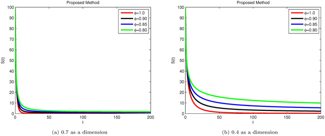
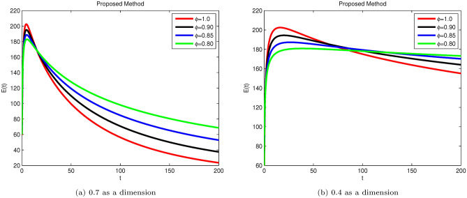
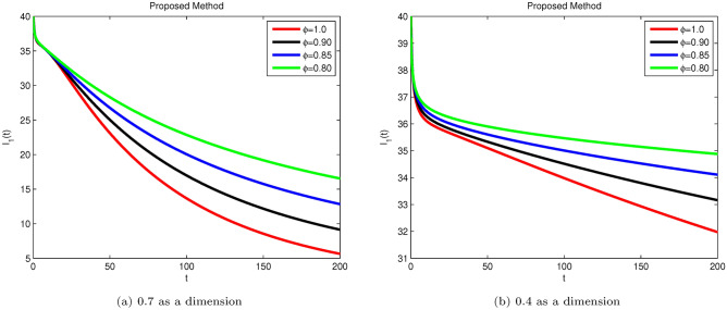
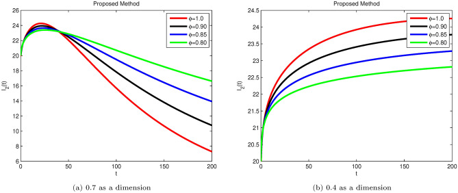
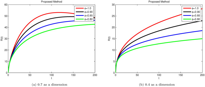
Here, we applied a sophisticated method to derive conceptual findings and evaluate their applicability. The following examples illustrate the validity of the theoretical results. The proposed $SE{I}_1{I}_{2}R$ system is explained using real situations through simulations. Figs. 3, 4, 5, 6, and 7 display the solutions for S(t), E(t), $I_1(t)$, $I_2(t)$, and R(t) for different fractional values across various dimensions. Numerical simulations for the Hepatitis B Virus model were conducted using MATLAB. The parameters used in the proposed system are as follows: $\rho =0.05$, $c=0.4$, $\eta =0.04$, ${\kappa }_0=0.03$, ${\kappa }_1=0.05$, ${\lambda }_1=0.06$, ${\lambda }_2=0.06$, $\delta =0.02$, $\lambda =0.03$, $\sigma =0.004$, with initial conditions: $S(0)=100$, $E(0)=60$, $I_1(0)=40$, $I_2(0)=20$, and $R(0)=0$.

Fig. 3.

Simulation of Hepatitis B sub-compartment S(t) with different fractional order value at dimensions 0.7 and 0.4.

Fig. 4.

Simulation of Hepatitis B sub-compartment E(t) with different fractional order value at dimensions 0.7 and 0.4.

Fig. 5.

Simulation of Hepatitis B sub-compartment $I_1(t)$ with different fractional order value at dimensions 0.7 and 0.4.

Fig. 6.

Simulation of Hepatitis B sub-compartment $I_2(t)$ with different fractional order value at dimensions 0.7 and 0.4.

Fig. 7.

Simulation of Hepatitis B sub-compartment R(t) with different fractional order value at dimensions 0.7 and 0.4.

Susceptible S(t), acutely infected $I_1(t)$, chronically infected $I_2(t)$, and recovered R(t) all decrease and approach a stable state over time, as seen in Figs. 3, 5, 6, and 7. The dynamics for E(t), representing asymptomatic cases identified early, rise as dimensions and fractional values decrease, stabilizing after some time, which can be seen in Fig. 4. Similar behaviors are observed whether using a dimension of 0.7 or 0.4, with minor effects; however, more appropriate results are achieved by reducing dimensions, as shown in Fig. 6a,b. These figures illustrate that acute infections start to reduce with a decrease in dimension while increasing with a dimension of 0.7. A comparison of fractional order with integer order results is presented in Fig. 3a, 4a, 5a, 6a, 7a and 3b, 4b, 5b, 6b, 7b, showing the graphical representation of HBV’s impact in acute and chronic stages using the suggested numerical method. Additionally, it is noted that as fractional values decrease, the solutions for each compartment become more reliable and accurate. Furthermore, it is observed that recovery increases with reduced fractional values and dimensions, as shown in Fig. 7a,b, under acute and chronic stages. Reducing dimension in HBV is to reduce the spread attack from different dimensions treated in the form like fractals. We need to minimize the effect from the different dimensions. This tells clearly that when dimensions are reduced, chronic stage infections are reduced as we observed in Fig. 6a,b part respectively. The order of the fractional derivative is utilized to investigate the continuous monitoring of the spread of HBV because the derivative tells us the rate of change of each sub-compartment of the HBV model. All derivative terms are included during formulations, and the fractional-order operator is used to investigate the continuous rate of change, which shows continuous monitoring of each sub-compartment. In contrast, the integer order provides investigation at a single point or within a single region. We provide detailed comparisons by taking fractional values 0.9, 0.85, and 0.80, and an integer order value of 1.0 to demonstrate how fractional operators capture the behavior of each sub-compartment for HBV more effectively and better capture the memory effects than the integer order. Similarly, we can observe the impact of asymptomatic measures, noting that acute infection $I_1$ and chronic infection $I_2$ reduce over time. Chronic infection, in particular, decreases sharply due to early detection measures and treatment. The parameters $\eta$ and $\gamma$ are most sensitive; if their rates increase, HBV spread increases. Conversely, if we decrease these parameters’ rates, HBV infections decrease, and ultimately, the system will become disease-free due to these control measures. If we raise the $\eta$ and $\rho$ rates from 0.05, HBV infection rises, causing liver cirrhosis due to an increase in the chronic stage. Therefore, it is crucial to maintain these rates through control measures. It is deduced that HBV can be controlled by combining early detection and treatment measures to manage liver infection in both acute and chronic stages.

Conclusion

We employ the sophisticated tool FFO for a fractional-order model of the viral illness hepatitis B to examine reliable data. This model is developed by incorporating both asymptomatic and treatment measures to control liver cirrhosis cases caused by HBV. For individuals with low immunity, we recommend strategies to prevent the spread of liver cirrhosis through early detection by introducing asymptomatic measures and chemotherapy treatment, which will help to make the environment disease-free soon. Examining the worldwide effects of chronic Hepatitis B virus (HBV) disease necessitates early risk factor detection and mitigation techniques. The constructed continuous dynamical system is analyzed qualitatively and statistically to evaluate its actual impact during chemotherapy to confirm its stability. It is necessary to understand how the model responds under constraints, which are established by both local and global stability analysis, to comprehend the dynamics of the epidemic. Additionally, we validate the presence of restricted and distinct solutions for the fractional-order HBV model, which are important characteristics to validate in newly created models. Furthermore, we determine the HBV’s bounded and positive solutions and examine the results of global initiatives to stop the virus’s spread and manage liver cirrhosis within the bounded domain. Prevention techniques and treatment approaches have demonstrated synergistic benefits that reduce the incidence of HBV infections and are beneficial in lowering the chronic stage of infection that results in liver cirrhosis. By using various fractional values, the FFO achieves trustworthy, practical results and continually monitors the progress under a continuous rate of change, including dimensions and control of the virus by combined measures. Numerical simulations using MATLAB are utilized to uncover the real behavior of the Hepatitis B virus in the population after exposure and chemotherapy within a regulated range of parameter $\eta$ and $\rho$ in order to prevent liver cirrhosis infection. Moreover, projections derived from verified outcomes could be employed in subsequent research to facilitate comprehension of the behavior and environmental dissemination of HBV, together with the early identification protocols.

Author contributions

Authors’ contributions Conceptualization; AA, MA, AHA. Writing - original draft preparation; AA, MA. Methodology; MAE-R, EH, HAN. Software and Visualization; AHA. Formal analysis and investigation; MAE-R, EH, HAN. Writing - review and editing: AHA, HAN. Resources; AA, MAE-R. Supervision: AA, AHA.

Data availability

The datasets used and/or analysed during the current study available from the corresponding author on reasonable request.

Ethical Approval

Not applicable.

Competing interests

The authors declare no conflict of interest.

References

- 1.WHO. Hepatitis B Fact Sheet No. 204 (The World Health Organisation, 2013). http://www.who.int/mediacentre/factsheets/fs204/en/.
- 2.Zada, I. et al. Mathematical analysis of hepatitis B epidemic model with optimal control. Adv. Differ. Equ.2021, 1–29 (2021). [Google Scholar]
- 3.World Health Organization. Unsafe Injection Practices Having Serious Large-Scale Consequences. Press Release WHO/14 (2000).
- 4.Mariano, A. et al. Role of beauty treatment in the spread of parenterally transmitted hepatitis viruses in Italy. J. Med. Virol.74(2), 216–220 (2004). [DOI] [PubMed] [Google Scholar]
- 5.Favero, M. S. & Bolyard, E. A. Microbiologic considerations: Disinfection and sterilization strategies and the potential for airborne transmission of bloodborne pathogens. Surg. Clin. N. Am.75(6), 1071–1089 (1995). [DOI] [PubMed] [Google Scholar]
- 6.Oda, Y. Women working at hairdressing: A case study of a rapidly increasing business among women in urban Ghana. Afr. Study Monogr.29, 83–94 (2005). [Google Scholar]
- 7.Khaliq, A. A. & Smego, R. A. J. Barber shaving and blood-borne disease transmission in developing countries: Issues in medicine: SAMJ forum. S. Afr. Med. J.95(2), 94–96 (2005). [PubMed] [Google Scholar]
- 8.World Health Organization. www.who.int/mediacentre/factsheets/fs204/en.
- 9.Candotti, D., Opare-Sem, O., Rezvan, H., Sarkodie, F. & Allain, J. P. Molecular and serological characterization of hepatitis B virus in deferred Ghanaian blood donors with and without elevated alanine aminotransferase. J. Viral Hepatitis13(11), 715–724 (2006). [DOI] [PubMed] [Google Scholar]
- 10.Kane, M. Global programme for control of hepatitis B infection. Vaccine13, S47–S49 (1995). [DOI] [PubMed] [Google Scholar]
- 11.Edmunds, W. J., Medley, G. F., Nokes, D. J., Hall, A. J. & Whittle, H. C. The influence of age on the development of the hepatitis B carrier state. Proc. R. Soc. Lond. Ser. B253(1337), 197–201 (1993). [DOI] [PubMed] [Google Scholar]
- 12.Medley, G. F., Lindop, N. A., Edmunds, W. J. & Nokes, D. J. Hepatitis-B virus endemicity: Heterogeneity, catastrophic dynamics and control. Nat. Med.7(5), 619–624 (2001). [DOI] [PubMed] [Google Scholar]
- 13.Ganem, D. & Prince, A. M. Hepatitis B virus infection natural history and clinical consequences. N. Engl. J. Med.350(11), 1118–1129 (2004). [DOI] [PubMed] [Google Scholar]
- 14.Brauer, F., Shuai, Z. & Van Den Driessche, P. Dynamics of an age-of-infection cholera model. Math. Biosci. Eng.10(6), 1335–1349 (2013). [DOI] [PubMed] [Google Scholar]
- 15.Huang, G., Liu, X. & Takeuchi, Y. Lyapunov functions and global stability for age-structured HIV infection model. SIAM J. Appl. Math.72(1), 25–38 (2012). [Google Scholar]
- 16.Rong, L., Feng, Z. & Perelson, A. S. Mathematical analysis of age-structured HIV-1 dynamics with combination antiretroviral therapy. SIAM J. Appl. Math.67(3), 731–756 (2007). [Google Scholar]
- 17.Franceschetti, A. & Pugliese, A. Threshold behaviour of a SIR epidemic model with age structure and immigration. J. Math. Biol.57(1), 1–27 (2008). [DOI] [PubMed] [Google Scholar]
- 18.O’Leary, C. et al. A mathematical model to study the effect of hepatitis B virus vaccine and antivirus treatment among the Canadian Inuit population. Eur. J. Clin. Microbiol. Infect. Dis.29, 63–72 (2010). [DOI] [PubMed] [Google Scholar]
- 19.Mann, J. & Roberts, M. Modelling the epidemiology of hepatitis B in New Zealand. J. Theor. Biol.269(1), 266–272 (2011). [DOI] [PubMed] [Google Scholar]
- 20.Thornley, S., Bullen, C. & Roberts, M. Hepatitis B in a high prevalence New Zealand population: A mathematical model applied to infection control policy. J. Theor. Biol.254(3), 599–603 (2008). [DOI] [PubMed] [Google Scholar]
- 21.Zou, L., Zhang, W. & Ruan, S. Modeling the transmission dynamics and control of hepatitis B virus in China. J. Theor. Biol.262(2), 330–338 (2010). [DOI] [PubMed] [Google Scholar]
- 22.Baleanu, D., Jajarmi, A., Mohammadi, H. & Rezapour, S. A new study on the mathematical modelling of human liver with Caputo-Fabrizio fractional derivative. Chaos Solitons Fractals134, 109705 (2020). [Google Scholar]
- 23.Defterli, O., Baleanu, D., Jajarmi, A., Sajjadi, S. S., Alshaikh, N., & Asad, J. H. Fractional Treatment: An Accelerated Mass-spring System (2022).
- 24.Khan, A. et al. Fractional dynamics and stability analysis of COVID-19 pandemic model under the harmonic mean type incidence rate. Comput. Methods Biomech. Biomed. Eng.25(6), 619–640 (2022). [DOI] [PubMed] [Google Scholar]
- 25.Raezah, A. A., Zarin, R. & Raizah, Z. Numerical approach for solving a fractional-order norovirus epidemic model with vaccination and asymptomatic carriers. Symmetry15(6), 1208 (2023). [Google Scholar]
- 26.Khan, A. et al. Modeling and sensitivity analysis of HBV epidemic model with convex incidence rate. Results Phys.22, 103836 (2021). [Google Scholar]
- 27.Khan, A., Zarin, R., Ahmed, I., Yusuf, A. & Humphries, U. W. Numerical and theoretical analysis of Rabies model under the harmonic mean type incidence rate. Results Phys.29, 104652 (2021). [Google Scholar]
- 28.Zarin, R., Khan, A., Akgul, A. & Akgul, E. K. Fractional modeling of COVID-19 pandemic model with real data from Pakistan under the ABC operator. AIMS Math.7(9), 15939–15964 (2022). [Google Scholar]
- 29.Gu, Y. et al. Mathematical analysis of a new nonlinear dengue epidemic model via deterministic and fractional approach. Alex. Eng. J.67, 1–21 (2023). [Google Scholar]
- 30.Alqhtani, M., Saad, K. M., Zarin, R., Khan, A. & Hamanah, W. M. Qualitative behavior of a highly non-linear Cutaneous Leishmania epidemic model under convex incidence rate with real data. Math. Biosci. Eng.21(2), 2084–2120 (2024). [DOI] [PubMed] [Google Scholar]
- 31.Yunus, A. O., & Olayiwola, M. O. The analysis of a novel COVID-19 model with the fractional-order incorporating the impact of the vaccination campaign in Nigeria via the Laplace-Adomian Decomposition Method. J. Niger. Soc. Phys. Sci. 1830 (2024).
- 32.Yunus, A. O., & Omoloye, M. A. Mathematical Analysis of Efficacy of Condom as a Contraceptive on the Transmission of Chlamydia Disease 22–37 (2022).
- 33.Olayiwola, M. O. & Yunus, A. O. Non-integer time fractional-order mathematical model of the COVID-19 pandemic impacts on the societal and economic aspects of Nigeria. Int. J. Appl. Comput. Math.10(2), 90 (2024). [Google Scholar]
- 34.Yunus, A. O., Olayiwola, M. O., Adedokun, K. A., Adedeji, J. A. & Alaje, I. A. Mathematical analysis of fractional-order Caputos derivative of coronavirus disease model via Laplace Adomian decomposition method. Beni-Suef Univ. J. Basic Appl. Sci.11(1), 144 (2022). [DOI] [PMC free article] [PubMed] [Google Scholar]
- 35.Yunus, A. O., Olayiwola, M. O., Omoloye, M. A. & Oladapo, A. O. A fractional order model of lassa disease using the Laplace-adomian decomposition method. Healthc. Anal.3, 100167 (2023). [Google Scholar]
- 36.Olayiwola, M. O., Alaje, A. I., Olarewaju, A. Y. & Adedokun, K. A. A Caputo fractional order epidemic model for evaluating the effectiveness of high-risk quarantine and vaccination strategies on the spread of COVID-19. Healthc. Anal.3, 100179 (2023). [DOI] [PMC free article] [PubMed] [Google Scholar]
- 37.Jajarmi, A. & Baleanu, D. A new fractional analysis on the interaction of HIV with CD4+ T-cells. Chaos Solitons Fractals113, 221–229 (2018). [Google Scholar]
- 38.Akgul, A., Li, C. & Pehlivan, I. Amplitude control analysis of a four-wing chaotic attractor, its electronic circuit designs and microcontroller-based random number generator. J. Circuits Syst. Comput.26(12), 1750190 (2017). [Google Scholar]
- 39.Lin, W. Global existence theory and chaos control of fractional differential equations. J. Math. Anal. Appl.332(1), 709–726 (2007). [Google Scholar]
- 40.Lemos-Paiao, A. P., Silva, C. J., & Torres, D. F. (2018). A cholera mathematical model with vaccination and the biggest outbreak of world’s history. arXiv preprint arXiv:1810.05823.
- 41.Baleanu, D., Ghassabzade, F. A., Nieto, J. J. & Jajarmi, A. On a new and generalized fractional model for a real cholera outbreak. Alex. Eng. J.61(11), 9175–9186 (2022). [Google Scholar]
- 42.Atangana, A. Mathematical model of survival of fractional calculus, critics and their impact: How singular is our world. Adv. Differ. Equ.2021(1), 403 (2021). [Google Scholar]
- 43.Lemos-Paiao, A. P., Maurer, H., Silva, C. J. & Torres, D. F. A SIQRB delayed model for cholera and optimal control treatment. Math. Model. Nat. Phenom.17, 25 (2022). [Google Scholar]
- 44.Van den Driessche, P. & Watmough, J. Reproduction numbers and sub-threshold endemic equilibria for compartmental models of disease transmission. Math. Biosci.180(1–2), 29–48 (2002). [DOI] [PubMed] [Google Scholar]
- 45.Vijayalakshmi, G. M. Vaccination control measures of an epidemic model with long-term memristive effect. J. Comput. Appl. Math.419, 114738 (2023). [DOI] [PMC free article] [PubMed] [Google Scholar]
Associated Data
This section collects any data citations, data availability statements, or supplementary materials included in this article.
Data Availability Statement