Research on low carbon welding scheduling based on production process

Abstract

The welding workshop of metal structural parts is highly energy-consuming. To meet the national low-carbon green demand, this paper focus on the welding workshop scheduling problem in production process with considering the carbon footprints such as equipment energy consumption, welding material consumption and shielding gas consumption. Firstly, a bi-objective low-carbon welding scheduling mathematical model is established with minimizing makespan and carbon emission. Then, an improved Grey Wolf Optimizer (IGWO) with three strategies is designed to solve this multi-objective problem. The grey wolf multi-wandering strategy (first) is proposed to enhance the population diversity. The grey wolf coordinated hunting strategy (second) based on dynamic weights is introduced to improve the convergence of IGWO. A local optimization strategy(third) is designed to improve the post-optimal search performance by adjusting the machine assignment based on the critical path. A welding workshop green scheduling case is designed to verify the model and algorithm proposed in this paper. The minimum completion time and carbon emissions obtained by the IGWO algorithm are 842.14 and 3.85E + 05, respectively. This result is better than that obtained by NSGA-II and GWO.The results show that the model effectively reduce the carbon emissions of the workshop, and the algorithm can effectively solve the model.

Supplementary Information

The online version contains supplementary material available at 10.1038/s41598-024-79555-0.

Introduction

In recent years, countries around the world have faced problems such as energy constraints and serious ecological degradation. The manufacturing industry consumes more than half of the country’s energy. As 80.7% of energy comes from coal and crude oil¹, the large amount of thermal power supply will certainly lead to the emission of CO₂ and other greenhouse gases into the environment². All these can lead to form an obvious greenhouse effect. At present, China’s manufacturing industry is the main driving force for the rapid development of the national economy. According to relevant statistics, the manufacturing industry consumes massive amounts of energy, and contributes to 36% of global CO₂ emissions³. As the main energy-consuming domain in China, the carbon emissions produced by the manufacturing industries are extremely huge. Therefore, it is quite significant for these industries to reduce the carbon emission. The welding plant is one of the main energy-consuming, so it is imperative to implement low-carbon and energy-saving scheduling optimization. Welding is widely used in industry such as astronautics, aviation, construction, shipbuilding, architecture, sluice locks and machinery manufacturing, etc. The potential on reducing carbon emission is huge. Reasonable arrangement of job sequence and the machine quantity can reduce the unnecessary energy consumption. It is of great practical significance for environmental protection and resource conservation.

The Welding Scheduling Problem (WSP) is widely studied with a strong engineering background and broad applications. The low-carbon WSP (LCWSP) is an extended flow shop scheduling problem (FSSP). At present, the researches on FSSP have abundant achievements. May et al.⁴ investigated the effects of production scheduling policies aimed towards improving productive and environmental performances in a job shop system. Yenisey and Yagmahan⁵ summarized and analyzed 86 literatures on multi-objective FSSP which identified opportunity areas of future research. The difference between WSP and FSSP is that it breaks the one-to-one correspondence of machine and job. The key feature is that a single job can be processed by multiple welding machines. Karaoglan A D⁶. provided an industrial application for the WSP under variable workstation constraints. Li X et al.⁷ investigated the extended FSSP with controllable processing time and established a multi-objective mathematical model on minimizing manufacturing cycle time and energy consumption. Wang et al.⁸ conducted research on distributed WSP based on the objectives of manufacturing energy consumption and manufacturing cycle time, which included three subproblems: inter-factory job allocation, intra-factory job scheduling and determining the machine number of each job. Wang et al.⁹ formulated a mathematical model of the welding shop inverse scheduling problem with the dynamic events and proposed an improved grey wolf optimizer (IGWO) for this problem. Lu C et al.¹⁰ addressed a human-robot collaborative WSP with minimization objectives of makespan and total energy consumption.

Some scholars have focused on low-carbon scheduling problems of industry workshops. Such as, Safarzadeh et al.¹¹ developed a green scheduling problem of uniform parallel machine environments with minimizing both total cost and makespan. Afsar et al.¹² studied the job shop scheduling problem with minimizing energy consumption and project makespan. Yin et al.¹³ conducted low-carbon scheduling research on flexible flow shop scheduling problems based on the analysis of carbon emissions in different states of machine tool operation. Tao et al.¹⁴ built a mathematical model to minimize the makespan, the total workload of machines and carbon emissions of machines, which could optimize the process method of each machine characteristic, process sequence and machine allocation at the same time. Zhang et al.¹⁵ established a mathematical model that simultaneously considered total energy consumption and total completion time minimum as the optimization objectives. This research studied the low-carbon distributed assembly and disassembly scheduling problem. Foumani M et al.¹⁶ presented a set of mathematical models, provided analysis and insights to design a framework of green FSSP. Yin et al.¹⁷ proposed a new low-carbon scheduling mathematical model from the perspective of reducing energy consumption and environmental pollution, optimizing productivity, energy efficiency and noise reduction. Tang et al.¹⁸ took the maximum completion time and total carbon emissions as the goal, and studied the green scheduling problem of the assembly flexible operation workshop. Jin et al.¹⁹ studied the problems related to carbon emissions in the auxiliary links of traditional flexible workshops, and gave corresponding solutions. Zhu et al.²⁰ considered the scheduling problem of low-carbon mixed assembly workshop in conjunction with AGV, and realized multi-objective optimization including carbon emissions. Jia et al.²¹ studied and explored the scheduling problem of green flexible job workshop, and introduced the relevant content of energy cost for modeling and solving. Li and Chen et al.²² took the flexible job workshop as the object, comprehensively considered the energy consumption and the learning effect of workers, and studied the existing green scheduling problems.

In summary, the flexible low-carbon scheduling problem and distributed low-carbon FSSP have been studied, but there is not much research on the LCWSPs. Most of the research objectives of the WSPs are machine load, manufacturing cycle time, welding energy consumption, but no consideration carbon footprint. The welding shop can generate variety carbon emission due to its complex production environment. Considering the carbon footprint of the actual welding process plays an important role in the research of LCWSP.

So, this paper studies the LCWSP based on the carbon footprint of the production process. This problem is a more complex multi-objective decision problem which should consider carbon emissions in addition to the traditional economic indicators. For this multi-objective scheduling problem, the traditional empirical-based production rules are difficult to obtain a better solution. The GWO²³ is an intelligence algorithm. All grey wolves are classified into four kinds according to their fitness values. The best wolf (solution) of GWO is denoted as the alpha (). Similarly, the second and third-best wolves are called beta ()and delta () respectively. The remaining wolves are . The search process is mainly guided by wolves , and , while the wolves should obey these three wolves. Eliminate the weak ones and renew the population through ‘survival of the fittest’ rule. The advantages of the GWO are clear: low sensitivity of algorithm parameters, strong global optimization ability, and simple algorithm design. Additionally, GWO performs very well on solving the practical application problems. This algorithm has been widely applied in continuous and combinatorial optimization problems such as TSP²⁴, workshop scheduling²⁵, path planning²⁶, and feature selection²⁷. But it has not yet ventured into the field of LCWSP.

This paper intends to study the LCWSP based on the carbon footprint of the production process. A low-carbon mathematical model to minimize the makespan and carbon emission is established. Given the complexity of this problem, an improved grey wolf algorithm (IGWO) should be designed to solve it.

Low carbon optimisation problem description and formulation

This section describes the LCWSP and presents a mathematical model which derives from a real-life welding shop.

Basic description of the LCWSP

This paper addresses a LCWSP which can be described as follows: n jobs must be processed through m stages in the same sequence, each job has only one operation at each stage. Preemption and interruption are not allowed. Multiple machines can operate the same job at the same time. Each machine can process at most only one job at the same time. Each operation has a determined processing time when only one machine is used to process the corresponding job. The processing time of each stage is negatively correlated with the number of machines, while the number at each operation is limited. Therefore, the task of the LCWSP is to find the optimal part process sequence and the optimal number of machines to handle the job at each stage to minimize processing time and carbon emission.

The processing process involves multiple times. Before welding, the job should be transported, which is known as the transport time. After it is transported to the designated location, the job needs to be preheated before welding. The processing time will be determined by the number of machines assigned to the stage. A Gantt chart illustration of a 3*3 example is as Fig. 1. Figure 1a represents a Gantt chart using single-machine welding, and Fig. 1b represents a Gantt chart using multi-machine welding.

Fig. 1.

Gantt chart comparison between welding single machine and multiple machines.

Mathematical models of LCWSP

If space permits, as many welding machines as possible should be arranged for each part. But we also know that more welding machines can lead to an increase in idle time, which in turn leads to an increase in carbon emission. Therefore, this article intends to construct a mathematical model based on the following assumptions and variables.

1. Assumptions:

   All jobs have the same welding process. Once a job is started by a machine, it cannot be interrupted. The number of machines for processing cannot be changed. Machine failures and the time required for setting the machine power are not considered. There is no priority among different jobs. The machines start working at time zero, and all machines are idle at time zero. Transport time and preheating time should be considered at each stage.

2. Nations:

   : the makespan of the welding

   : a feasible sequence

   : job position of the sequence

   : index of job and stage respectively

   : the quantity of jobs and stages respectively

   : operation of job at stage

   : maximum number of welding equipment for the job at stage

   : carbon emission factor of electric energy, welding material, and shielding gas respectively

   : power of handling equipment, power of preheating equipment before welding of job at stage

   : lifting time, a preheating time before welding of job at stage

   : actual welding power and standby power of the welding equipment of the job at stage

   : normal welding time of job at stage

   : welding material consumption per unit time of a single welding machine

   : consumption of shielding gas per unit time of a single welding machine

   : power of auxiliary production equipment per unit time

3. Variables:

   : actual welding time of job at stage

   : completion time of job at stage

   : welding start time of job at stage

   Decision variables:

   : the number of machines occupied by job at the stage

   

4. Analysis of welding shop carbon footprint.

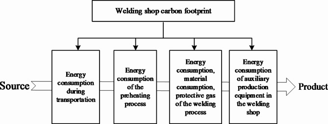
   The carbon footprint of the welding workshop is considered and analyzed from the perspective of welding process, concerning the dividing means of carbon emission accounting boundary and the corresponding calculation methods^28–31. All these papers are related to low-carbon manufacturing and scheduling problems. In this paper, the carbon footprint of the welding workshop will consider the energy consumption of transportation equipment, welding preheating equipment, welding equipment, welding material consumption, welding protective gas generation, and auxiliary production equipment (in Fig. 2).

   With the above notations and carbon footprint analysis, the mathematical model of the welding carbon emission can be formulated as follows:

   1

   2

   3

   4
   Wherein,

   5

   6

   7

   Equation (1) gives the carbon emissions of the transport process. Equation (2) expresses the carbon emissions of the preheating process before welding. Equation (3) denotes the carbon emissions generated by the auxiliary production equipment. Equation (4) means the carbon emissions from the welding process. Equation (5) defines the carbon emissions of the welding consumption. Equation (6) shows the energy consumption of welding equipment, including standby and working energy consumption. Equation (7) is the consumption of shielding gas.

5. The mathematical model of LCWSP can be formulated as follows:

   Objectives:

   8

   9
   Constraints:

   10

   11

   12

   13

   14

   Equations (8) and (9) denote the objective to minimize makespan and carbon emissions. Constraint (10) imposes that the number of available machines to process each operation should obey its respective range. Constraint (11) ensures that a job can be processed at most one stage at the same time. Constraints (12) and (13) can guarantee each job not be started until its preceding operations are completed and the job is available at the next stage. Constraint (14) specifies that the makespan is the machining completion time of the last job.

Fig. 2.

Carbon footprint of welding shop.

Improved Grey Wolf Optimizer

In this paper, an IGWO is proposed for the LCWSP with double-layer coding. A combination of random initialization and NEH method is implied to initialize the population. The wandering and running behaviors of grey wolves are redesigned based on the traditional GWO. A local optimization strategy is introduced to adjust the vector of assigned machines according to the critical path. Just as follows:

Decimal integer encoding and decoding scheme

The representative discrete combinatorial optimization problem is divided into two sub-problems: job sequence and machine quantity allocation. The coding is also composed of job sequence and machine quantity allocation. In this paper, the decimal integer encoding method is designed to express the job sequence and the number of machines assigned to each stage of the job.

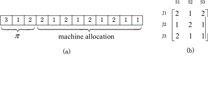
Different coding and decoding methods perform an impact on the efficiency of the algorithm. Considering the convergence speed and search space of the algorithm, this paper adopts the coding structure shown in Fig. 3. The total length of the encoding is the sum of the job number and the machine allocation vector.

Fig. 3.

Example of encoding.

The sequence of the job is the decimal sequence from left to right. As shown in Fig. 3a. The first part of the solution vector indicates that job 3, job 1 and job 2 are processed sequentially. The second part of the solution vector represents the number of welding machines allocated at each stage of each workpiece. Wherein, indicates that job 3 is allocated 2 welding machines at stage 1, the same is true for and so on. In addition, Fig. 3b represents the number of machines assigned to each workpiece at different stages.

Random and NEH initialization method

To improve the solution quality and evolution speed, the present study employs two methods, namely random and NEH initialization, to generate initial population. The entire initialization population represents the solution space of the LCWSP, and each solution means a feasible scheduling scheme.

Multi-wandering search strategy for the prey

Grey wolves wander to search for prey, can be understood as searching for the optimal solution in the solution space. The wolves keep approaching α wolf during the evolution process, which may be easy to fall into the local optimum due to that the α wolf is not necessarily at the global optimum. The original GWO has two coefficients to adjust the search direction to avoid getting into local optima. A multi-wandering search strategy is designed based on the characteristics of the discrete IGWO and the low-carbon scheduling problem, mainly used to expand the search range of Grey Wolf.

The grey wolf searches for prey through wandering behavior, which can be understood as searching for the optimal solution. The basic idea is to systematically change the structure and expand the search range during the search process to obtain an optimal solution. This search strategy performs better optimization ability.

To address the characteristics of the solution model in this paper, three random search mechanisms are designed, which will involve changing the sequence of jobs and the allocation of machines in a feasible scheduling plan according to certain rules. Specifically, the mechanisms are as follows.

1. Exchange the processing sequence of jobs and the allocation of machines in a feasible scheduling plan. Select two elements from the job sequence randomly and exchange them. The same operation on the machine allocation sequence is performed. As shown in Fig. 4a.

2. Chose a certain scheduling plan, randomly select two nonadjacent elements. Then, reverse the elements between the two elements. The same operation is performed on the machine allocation sequence to obtain a new wolf. As shown in Fig. 4b.

3. Move two adjacent jobs in one solution to other positions together. That is, randomly select two adjacent positions, select a job from the solution as the insertion node, keep the adjacency after the movement. Perform the same operation on the machine allocation sequence, as shown in Fig. 4c.

   After executing the wandering strategy, the objectives are compared with the grey wolf, the inferior grey wolves are eliminated, and a new population of grey wolves are formed.

Fig. 4.

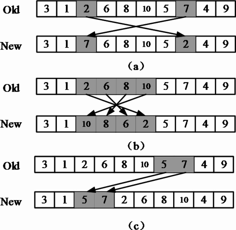
Grey wolf search strategy.

Coordinated hunting strategy

After wandering, the exploring wolf transforms into a fierce wolf, and the head wolf howls to summon the fierce wolf, directing them to approach the location of their prey and engage in hunting.

The coordinated hunting behavior is the process of wolves approaching the prey position under the guidance of the leading wolves. After the grey wolves wandered, the wolf pack is sorted into layers according to the Pareto relationship³² based on the objectives in this article. The leading wolf are selected as the leaders randomly while the other wolves become hunting wolves. In the original GWO, the explorers update their positions based on the positions of the head wolf, the impact of three wolves on other wolves is the same, and the important influence of the optimal wolf is not reflected. The random selection of the three wolves will affect the convergence speed of the algorithm. To improve the convergence of the algorithm, this article proposes a dynamic weight strategy that enhances the role of the best wolf and reduces the roles of the other two wolves during the iteration process. The weight expression can be represented as Eq. (15):

15

Where , and represent the fitness of the three wolves, respectively. As the algorithm iterates, the fitness values gradually decrease, and the weight values gradually change. Among the three leading wolves, the wolf has the highest probability to be chosen, followed by the wolf . The dynamic weight-hunting strategy designed in this article strengthens the role of the best wolf during the continuous search process, which can improve the convergence of the algorithm.

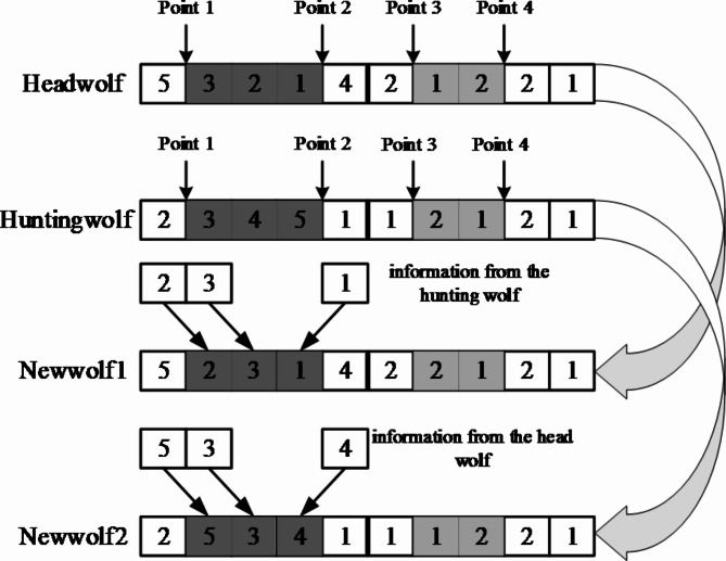
The specific process of grey wolf cooperative hunting is as follows: The hunting wolf chooses a lead wolf based on the dynamic weight strategy. It cooperates with the selected wolf to hunt the prey by exchanging information through multi-point interaction. The process is illustrated in Fig. 5.

Fig. 5.

The hunting behavior of grey wolves.

Assuming that the second, fourth, seventh, and eighth encoding positions are randomly selected as interaction points for information exchange. With the second and fourth positions, the hunting is conducted through information exchange. The interaction codes of lead wolf are {3, 2, 1}, which are replaced by the corresponding position order of hunt wolf (the job sequence in the hunt wolf). The interaction codes selected from hunt wolf are {3, 4, 5}, which should be replaced by the corresponding position order of lead wolf. The seventh and eighth codes represent the machine allocation encoding sequence, which will hunt through a crossover method.

Adjust the vector of assigned machines according to the critical path

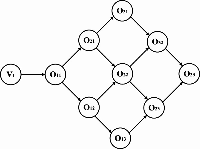
Based on the actual production of the welding shop, it can be known that the job can be welded by multiple machines, which can advance the completion time. However, it may cause an increase of carbon emissions. Therefore, finding the appropriate number of welding machines to balance the makespan and carbon emissions is crucial. In this paper, the Activity On Edge (AOE) network diagram structure is generated based on the sequence of jobs and the sequence of stages. As shown in Fig. 6, represents the source point, represents the completion, and the edge represents the time required to complete the process. Topological sorting is used to calculate the earliest and latest start time of the process. Find out the critical path, increase the number of machines assigned on it. Correspondingly, reduce the number of machines assigned on the non-critical path.

Fig. 6.

The AOE network diagram structure.

During the iteration, it is difficult to further reduce the objective value by adjusting the jobs sequence after the iteration number reaches a certain point. At this point, the machine assignment sequence can be adjusted by referring to the critical path. As the machines number of non-critical path is reduced, the processing time of this stage, the makespan, and the carbon footprint are all reduced.

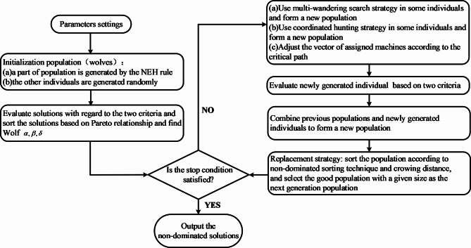
The procedure of IGWO

The procedure of the proposed IGWO is shown in Fig. 7.

Fig. 7.

Procedure of the proposed IGWO.

Experimental design and results discussion

This section is devoted to measure the performance of the proposed IGWO for the addressed problem. All algorithms are coded by the Matlab R2020A software. The experimental environment for this article is a computer with Intel(R) Core (TM) i9-13900 K, 3.00 GHz, 128GB RAM, with a Windows 10 64-bit system. To verify the performance of the proposed algorithm in this paper, different scale test examples are designed for the problem. The IGWO is simulated and compared with GWO and NSGA-II under different scale examples. The feasibility and superiority of the proposed algorithm are verified. Finally, the production data of an enterprise is used as a practical case to verify the algorithm. Except for special instructions, the stopping criterion with CPU time is set as seconds.

Performance metrics

To measure the Pareto Front obtained by these multi-objective evolutionary algorithms, three metrics including NR, GD, and IGD should be employed below.

1. Rate of Non-dominated Solutions (NR). This metric reflects the proportion to the reference solution set of the algorithm. The larger the NR value, the higher the proportion of the non-dominated solutions obtained by the algorithm, which indicates better performance and more scheduling options available.

2. Generational Distance (GD). The GD evaluates the nearest distance between the approximate optimal solution obtained by one algorithm and the Pareto Front solutions. The smaller value, the stronger convergence of the solutions.

3. Inverse Generational Distance (IGD). The IGD is a variant of the GD, which can simultaneously evaluate both convergence and diversity. This metric can measure the mean Euclidean Distance between reference solutions at the Pareto Front and the nearest algorithm solution.

Result comparison and discussion

To verify the effectiveness of the improved algorithm, simulation experiments are conducted by different sizes of arithmetic cases. Table 1 shows the distribution of test cases of the simulation experiments. Each case is solved 10 times by the GWO, NSGA-II and the IGWO of this paper, respectively. To evaluate and analyze the solution performance of each algorithm for LCWSP, the three indicators mentioned above are introduced to evaluate the performance of the algorithms. Through several experiments, taking into account the quality of the solution and the speed of the solution, the parameters of IGWO are set as follows:, ,, initialize external storage ∅, NSGA-II (with parameters set according to reference³³, the traditional GWO (with parameters set the same as the IGWO). Three algorithms respectively solve the mathematical model established in this article.

Table 1.

The distribution of test examples.

Variables	Value or distribution
Job number	10, 20, 30, 40, 50, 60
Stage number	3, 5, 10
Max number of available machines per stage	U[1, 4]
Welding time	U[8, 20]
Transport time	U[2, 5]
Preheat time	U[1, 3]

Table 2 shows the comparison of NR, GD, and IGD metric values. The NR index of IGWO proposed in this paper is stronger than NSGAII and GWO in most cases. Although there is not much different performance for small-scale problems, as the scale of the problem increases, the performance of the IGWO is significantly better than other algorithms. All these performances indicate that the solution obtained by IGWO is closer to the true Pareto Front.

Table 2.

Comparative analysis of algorithm operation results.

Example	IGWO			NSGA-II			GWO
	NR	GD	IGD	NR	GD	IGD	NR	GD	IGD
10*3	0.36	1.20E – 02	5.64E – 02	0.36	1.29E – 02	9.84E – 02	0.3	2.15E – 02	1.40E – 01
20*3	0.35	1.05E – 02	4.05E – 02	0.34	1.61E – 02	1.40E – 01	0.32	4.04E – 02	1.98E – 01
30*3	0.37	9.50E – 03	3.98E – 02	0.32	1.40E – 02	1.53E – 01	0.35	3.74E – 02	2.99E – 01
40*3	0.38	9.90E – 03	6.86E – 02	0.34	1.52E – 02	1.90E – 01	0.29	3.57E – 02	2.57E – 01
50*3	0.40	6.20E – 03	4.74E – 02	0.31	9.90E – 03	1.48E – 01	0.31	1.63E – 02	2.43E – 01
60*3	0.39	9.00E – 03	5.53E – 02	0.36	3.56E – 02	3.22E – 01	0.3	4.06E – 02	2.98E – 01
10*5	0.39	1.59E – 02	6.07E – 02	0.38	2.09E – 02	2.00E – 01	0.26	3.89E – 02	2.46E – 01
20*5	0.45	8.60E – 03	5.48E – 02	0.44	1.06E – 02	3.10E – 01	0.16	2.69E – 02	2.26E – 01
30*5	0.38	1.03E – 02	6.73E – 02	0.36	1.26E – 02	2.99E – 01	0.32	2.43E – 02	2.16E – 01
40*5	0.38	1.26E – 02	5.99E – 02	0.37	1.69E – 02	2.68E – 01	0.25	2.96E – 02	2.40E – 01
50*5	0.39	5.70E – 03	6.99E – 02	0.38	2.64E – 02	2.70E – 01	0.24	3.01E – 02	2.80E – 01
60*5	0.45	8.30E – 03	1.11E – 01	0.39	3.20E – 02	3.51E – 01	0.17	4.29E – 02	2.58E – 01
10*10	0.36	3.04E – 02	1.02E – 01	0.34	4.05E – 02	3.63E – 01	0.32	4.12E – 02	2.40E – 01
20*10	0.46	9.90E – 03	7.01E – 02	0.3	1.02E – 02	2.45E – 01	0.29	1.50E – 02	2.11E – 01
30*10	0.43	7.50E – 03	9.22E – 02	0.32	2.71E – 02	3.12E – 01	0.26	2.99E – 02	3.10E – 01
40*10	0.5	2.03E – 02	5.97E – 02	0.35	3.20E – 02	3.11E – 01	0.17	4.32E – 02	2.29E – 01
50*10	0.56	1.06E – 02	8.91E – 02	0.36	1.41E – 02	4.05E – 01	0.16	2.56E – 02	3.62E – 01
60*10	0.57	9.90E – 03	6.45E – 02	0.34	2.24E – 02	2.45E – 01	0.18	3.29E – 02	2.31E – 01

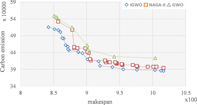
Comparing the GD values in Table 2, IGWO is smaller than NSGA-II and GWO in most cases, which shows that IGWO performs better convergence than the compared algorithms. For the IGD values, the performance of the solutions obtained by the IGWO is better than the other two compared algorithms, which proves that the multi-wandering search strategy proposed in this paper can expand the search scope. From the Pareto Front plots of the three algorithms described in Fig. 8, the front of IGWO is better than that of NSGA-II. The solution effect of IGWO is much better than that of GWO due to the design of the search for prey strategy, the dynamic weighted cooperative hunting strategy, and the critical path-based machine number adjustment strategy, which is consistent with the data in Table 2.

Fig. 8.

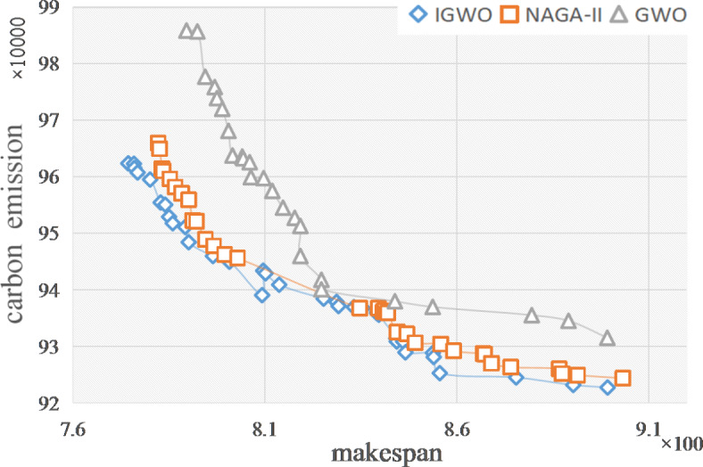
Pareto Front of three algorithms.

Target analysis and algorithm strategy comparison

To verify the superiority of the model, this paper takes a 10*5 welding example, and compares the carbon emissions obtained by considering only the makespan with the dual goals. The results are shown in Table 3.

Table 3.

Comparison of carbon emission results.

Number	Consider the makespan		Consider the carbon emissions and the makespan
	Makespan	Carbon emission	Makespan	Carbon emission
1	407.79	119507.4733	425.11	118492.3519
2	410.16	119493.3306	425.89	118475.6643
3	412.26	119396.6594	432.84	118346.8221
4	413.42	119366.4742	441.53	118266.9058
5	416.79	119349.7736	448.81	118088.7119
6	418.02	118960.2269	450.68	118022.1879
7	420.32	118862.7169	452.26	117625.1915
8	424.44	118812.8145	461.47	117504.0569

It can be found that the carbon emissions of a single objective model will be much higher than those of a multi-objective model. The dual-objective model established in this paper significantly reduces carbon emissions at the small expense of makespan.

To compare the optimization effect of the three strategies, the results obtained when only two of the strategies are used are shown in Table 4.

Table 4.

The significant comparison of the three strategies.

Number	No first strategy		No second strategy		No third strategy
1	860.89	4.98E + 05	991.26	3.99E + 05	984.11	4.01E + 05
2	884.62	4.79E + 05	921.63	4.32E + 05	886.84	4.85E + 05
3	954.39	4.22E + 05	848.24	5.11E + 05	1001.82	3.89E + 05
4	995.63	4.07E + 05	1005.36	3.92E + 05	964.41	4.22E + 05
5	845.39	5.09E + 05	891.71	4.66E + 05	857.58	5.00E + 05
6	926.72	4.56E + 05	856.49	5.09E + 05	846.22	5.09E + 05
7	1023.11	3.86E + 05	886.74	4.72E + 05	927.10	4.52E + 05
8	971.32	4.16E + 05	902.34	4.41E + 05	907.48	4.77E + 05

Significant values are in bold.

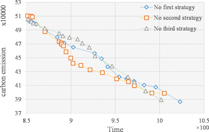
The comparison of the three strategies in Table 4 shows that the three strategies have a certain impact on the performance of the algorithm. From the data obtained, it can be seen that when the grey wolf multi-wandering strategy(first strategy) is not available, the maximum time to completion and carbon emissions tend to increase slightly. When the grey wolf coordinated hunting strategy(second strategy) is not adopted, it does not always lead to worse outcomes compared to the other two strategy. On the other hand, when a local optimization strategy(third strategy) is not introduced, the algorithm will deteriorate significantly in most cases. A comparison of the Pareto fronts of the three strategies is shown in Fig. 9.

Fig. 9.

Pareto Front comparison of three strategies.

Practical case application

To further verify the effectiveness of the IGWO and mathematical model proposed in this paper, the welding task of a certain mechanical and shipbuilding company was selected as the research object. The relevant data are simplified as Table 5. Each algorithm was randomly run 10 times and the excellent solutions were selected for comparison, with the optimal results highlighted in bold in Table 6. To analyze the differences more intuitively among the three algorithms, the Pareto Front distribution of the three algorithms was described in Fig. 10.

Table 5.

Scheduling tasks of welding workshop.

Job	Stage
	12/3/60	24/10/280	3/5/37	16/17/76	7/8/25	14/15/67	10/10/41	7/7/18
	13/5/65	23/16/200	10/15/16	25/18/90	10/12/29	14/11/60	14/15/67	25/20/61
	9/3/55	19/7/207	7/6/27	17/16/70	15/17/48	14/14/71	22/10/56	12/14/28
	10/4/57	26/5/259	9/15/57	27/10/68	10/17/41	14/4/47	10/18/30	22/14/44
	6/6/65	30/8/212	7/20/48	16/17/96	15/22/52	18/7/60	14/10/27	5/3/9
	5/9/78	12/9/180	20/16/51	20/5/53	20/24/34	16/16/74	13/10/70	5/7/13
	9/3/46	15/10/260	16/13/24	14/25/55	20/15/45	13/17/42	9/8/34	25/26/63

Table 6.

Results comparative analysis of three different algorithms.

Number	IGWO		NSGA-II		GWO
1	842.14	5.15E + 05	878.18	5.08E + 05	1004.02	4.23E + 05
2	851.37	5.09E + 05	1005.74	3.98E + 05	941.70	4.28E + 05
3	920.30	4.00E + 05	880.96	4.56E + 05	901.93	4.49E + 05
4	955.42	3.90E + 05	856.95	5.32E + 05	900.81	4.61E + 05
5	918.21	4.14E + 05	969.82	4.03E + 05	877.77	5.15E + 05
6	1016.39	3.85E + 05	903.07	4.39E + 05	855.32	5.43E + 05
7	1003.49	3.88E + 05	1016.39	3.94E + 05	850.72	5.49E + 05
8	871.79	4.50E + 05	905.12	4.21E + 05	853.49	5.46E + 05

Fig. 10.

Pareto Front comparison of three algorithms.

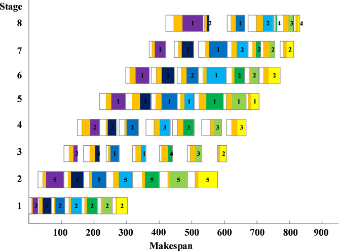
The comparison of the algorithms in Table 6; Fig. 11 shows that in terms of maximum completion time, the results obtained by the IGWO algorithm are reduced by 1.73% and 1.01% compared with the NSGA-II and the GWO, respectively. For carbon emissions, the results obtained by the IGWO algorithm are 2.28% and 8.98% lower than those obtained by the NSGA-II and the GWO, respectively. Therefore, the IGWO used in this paper can achieve better result than the other two algorithms, and can obtain the optimal values of the optimization objectives.

Fig. 11.

The Gantt chart of the real-life case.

The IGWO used in this paper adopts three strategies, which are improved in three aspects: initial population diversity, algorithm convergence, and local optimization in the later stage. The improved algorithm can best solve the LCWSP.

The numbers on the Gantt chart in Fig. 11 represent the numbers of machines assigned at each stage of the job. The maximum number of machines available in the second stage is too small, resulting in the makespan cannot be further optimized. The workshop can increase the number of welding machines available in the second stage and shorten the makespan.

Conclusions and future work

This paper considers the carbon footprint caused by equipment energy consumption, welding material consumption and protective gas consumption during the production process of welding workshops. The LCWSP mathematical model is established to minimize the makespan and carbon emission.

The IGWO is designed to solve the research problem in this paper. High-quality initial populations are formed through a combination of random generation and NEH strategies. To balance the effect of global and local search, three strategies were designed. The first is the multi-wandering search strategy, the second is grey wolf cooperative hunting strategy with dynamic weights. The third is to adjust the number of machine allocations on the critical path. The resulting excellent specimen is preserved through external memory.

Test cases are generated based on actual welding shop production. By using three different algorithms, it shows that the results obtained by IGWO are better than those of other two algorithms. In terms of maximum completion time, the results obtained by IGWO algorithm are reduced by 1.73% and 1.01%, respectively, compared with NSGA-II and GWO. For carbon emissions, the results obtained by the IGWO algorithm are 2.28% and 8.98% lower than those of NSGA-II and GWO, respectively. These comparison results show the advantages of the proposed algorithm in population initialization and optimization, and an example application verifies the effectiveness of the IGWO on solving the multi-objective LCWSP.

In addition, the relevant results in this paper can provide a reference for enterprise dispatchers, help enterprises formulate green production scheduling plans, and reduce carbon emissions in the production process. The limitation of this paper is that the relevant consideration of the sources of carbon emissions is not complete, such as the carbon emissions generated during the aging treatment after welding. In the future, the low-carbon scheduling problem of distributed welding workshops will be studied with considering more practical constraints, and to further improve the algorithm accordingly.

Electronic supplementary material

Below is the link to the electronic supplementary material.

Author contributions

F.G. contributes equally with the first author R.M.: Writing–review, editing, Supervision; ZY.W.: Software, Writing–original draft, Methodology, Writing–review, editing; W.Z.: Conceptualization, Writing–review, editing; D.L.: Editing, Methodology; ZJ.W.: Editing; S.D.: Editing; All authors reviewed the manuscript.

Funding

This work is financially supported by Natural Science Foundation of Hubei Province (No.2022CFC033), the National Natural Science Foundation of China (No.52205575), 2022 graduate course construction and cultivation project of China Three Gorges University (No. SDKC202203), and Yichang Natural Science Research Project(A23-2-006).

Data availability

The data files used in the manuscript have been uploaded to a supplementary file. Some of the data is the research data from the enterprise, and therefore it is not publicly available. However, it may be obtained from the corresponding author upon reasonable request.

Declarations

Competing interests

The authors declare no competing interests.

References

- 1.Zhang, R. & Chiong, R. Solving the energy-efficient job shop scheduling problem: a multi-objective genetic algorithm with enhanced local search for minimizing the total weighted tardiness and total energy consumption. J. Clean. Prod., 112, 3361–3375. 10.1016/j.jclepro.2015.09.097.
- 2.Lu, C. et al. A pareto-based hybrid iterated greedy algorithm for energy-efficient scheduling of distributed hybrid flowshop. Expert Syst. Appl.204, 117555. 10.1016/j.eswa.2022.117555 (2022). [Google Scholar]
- 3.Mansouri, S. A., Aktas, E. & Besikci, U. Green scheduling of a two-machine flowshop: Trade-off between makespan and energy consumption. Eur. J. Oper. Res.248 (3), 772–788 (2016). [Google Scholar]
- 4.May, G. et al. Multi-objective genetic algorithm for energy-efficient job shop scheduling. Int. J. Prod. Res.53 (23), 7071–7089. 10.1080/00207543.2015.1005 (2015). [Google Scholar]
- 5.Yenisey, M. M. & Yagmahan, B. Multi-objective permutation flow shop scheduling problem: Literature review, classification, and current trends. Omega, 45, 119–135. (2013). 10.1016/j.omega. 07.004 (2014).
- 6.Karaoglan, A. D. Optimization of welding job-shop scheduling problem under variable workstation constraint: an industrial application with Arena simulation based genetic algorithm. Pamukkale Üniversitesi Mühendislik Bilimleri Dergisi. 28 (1), 139–147 (2022). [Google Scholar]
- 7.Li, X. et al. An effective multiobjective algorithm for energy-efficient scheduling in a real-life welding shop. IEEE transactions on industrial informatics, 14(12), 5400–5409. (2018). 10.1109/TII.2018. 2843441.
- 8.Wang, G. et al. An effective multi-objective whale swarm algorithm for energy-efficient scheduling of distributed welding flow shop. Ann. Oper. Res.310 (1), 223–255. 10.1007/s10479-021-03952-1 (2022). [Google Scholar]
- 9.Wang, C. et al. An improved grey wolf optimizer for welding shop inverse scheduling. Comput. Ind. Eng.163, 107809. 10.1016/j.cie.2021.107809 (2022). [Google Scholar]
- 10.Lu, C. et al. Human-Robot Collaborative Scheduling in Energy-efficient Welding Shop. IEEE Trans. Industr. Inf.10.1109/TII.2023.3271749 (2023). [Google Scholar]
- 11.Safarzadeh, H. & Niaki, S. T. A. Bi-objective green scheduling in uniform parallel machine environments. J. Clean. Prod.217, 559–572. 10.1016/j.jclepro.2019.01.166 (2019). [Google Scholar]
- 12.Afsar, S. et al. Multi-objective enhanced memetic algorithm for green job shop scheduling with uncertain times. Swarm Evol. Comput.68, 101016. 10.1016/j.swevo.2021.101016 (2022). [Google Scholar]
- 13.Yin, R. et al. Flexible Flow Shop Scheduling and Energy Saving Optimization Strategy under Low Carbon Target//Journal of Physics: Conference Series. IOP Publishing, 012095. (1939). 10.1088/1742-6596/1939/1/012095 (2021).
- 14.Ning, T. et al. Research on flexible job shop scheduling with low-carbon technology based on quantum bacterial foraging optimization. Int. J. Low-Carbon Technol.16 (3), 761–769. 10.1093/ijlct/ctab005 (2021). [Google Scholar]
- 15.Zhang, Z. et al. Multidimensional estimation of distribution algorithm for low carbon scheduling of distributed assembly permutation flow-shop. Control Decis.37 (05), 1367–1377. 10.13195/j.kzyjc.2020.1475 (2022). [Google Scholar]
- 16.Foumani, M. & Smith-Miles, K. The impact of various carbon reduction policies on green flowshop scheduling. Appl. Energy. 249, 300–315. 10.1016/j.apenergy.04.155 (2019). [Google Scholar]
- 17.Yin, L. et al. A novel mathematical model and multi-objective method for the low-carbon flexible job shop scheduling problem. Sustainable Computing: Inf. Syst.13, 15–30. https://doi.org/suscom.2016.11.002 (2017). [Google Scholar]
- 18.Tang, H. et al. Improved artificial bee colony algorithm based on Q-learning to solve the green scheduling problem of distributed assembly flexible operation workshop.Industrial Engineering and Management,1–22. (1939). http://kns.cnki.net/kcms/detail/31.1738.T.20240701.006.html. (2024).
- 19.Jin, Z. et al. Combined with NSGA-II.‘s flexible workshop low-carbon Scheduling. Mod. Manuf. Eng.05, 6–14. 10.16731/j.cnki.1671-3133.2023.05.002 (2023). [Google Scholar]
- 20.Zhu, G., Jia, W. & Li, D. Research on the scheduling of low-carbon mixed assembly line workshop combined with AGV and machine.Journal of Beijing University of Aeronautics and Astronautics,1–15. (2024). 10.13700/j.bh.1001-5965.2023.0021
- 21.Jia, S. et al. The Green Flexible Job-Shop Scheduling Problem Considering Cost, Carbon Emissions, and Customer Satisfaction under Time-of-Use Electricity Pricing.Sustainability,16(6). (2024).
- 22.Zhi, L. & Yingjian, C. Minimizing the makespan and carbon emissions in the green flexible job shop scheduling problem with learning effects. Sci. Rep.13 (1), 6369–6369 (2023). [DOI] [PMC free article] [PubMed] [Google Scholar]
- 23.Mirjalili, S., Mirjalili, S. M. & Lewis, A. Grey wolf optimizer. Adv. Eng. Softw.69, 46–61. 10.1016/j.advengsoft.2013 (2014). 12.007. [Google Scholar]
- 24.Panwar, K. & Deep, K. Discrete Grey Wolf Optimizer for symmetric travelling salesman problem. Appl. Soft Comput.105, 107298. 10.1016/j.asoc.2021.107298 (2021). [Google Scholar]
- 25.Meng, R. et al. Research on Complex Hybrid Flow-Shop Scheduling Problem solved by Improved Grey Wolf Optimizer. Acta Electronica Sinica. 49 (08), 1515–1523. 10.12263/DZXB.20191319 (2021). [Google Scholar]
- 26.Jarray Raja, A. D., Mujahed, R. & Hegazy Bouallègue Soufiene. Parallel Cooperative Coevolutionary Grey Wolf Optimizer for Path Planning Problem of Unmanned Aerial Vehicles. Sensors, 22(5). (2022). 10.3390/s22051826 [DOI] [PMC free article] [PubMed]
- 27.Shen, C. & Zhang, K. Two-stage improved Grey Wolf optimization algorithm for feature selection on high-dimensional classification. Complex. Intell. Syst. 1–21. 10.1007/s40747-021-00452-4 (2022).
- 28.Pandey, D., Agrawal, M. & Pandey, J. S. Carbon footprint: current methods of estimation. Environ. Monit. Assess.178, 135–160. 10.1007/s10661-010-1678-y (2011). [DOI] [PubMed] [Google Scholar]
- 29.Zhang, C. & Ji, W. Digital twin-driven carbon emission prediction and low-carbon control of intelligent manufacturing job-shop. Procedia CIRP, 83, 624–629. (2019). 10.1016/j.procir. 04.095 (2019).
- 30.Liao, W. & Wang, T. A novel collaborative optimization model for job Shop production–delivery considering time window and carbon emission. Sustainability, 11(10), 2781. (2019). 10.3390/su11102781
- 31.Li, N., Wang, X. & Bai, Y. An improved genetic algorithm for low carbon dynamic scheduling in a discrete manufacturing workshop.//Journal of Physics: Conference Series. IOP Publishing, 1820(1), 012111. (2021). 10.1088/1742-6596/1820/1/012111
- 32.Lu, C. et al. A pareto-based collaborative multi-objective optimization algorithm for energy-efficient scheduling of distributed permutation flow-shop with limited buffers. Robot. Comput. Integr. Manuf.74, 102277. 10.1016/j.rcim.2021.102277 (2022). [Google Scholar]
- 33.Deb, K. et al. A fast and elitist multi objective genetic algorithm: NSGA-II. IEEE Trans. Evol. Comput.6 (2), 182–197. 10.1109/4235.996017 (2002). [Google Scholar]
Associated Data
This section collects any data citations, data availability statements, or supplementary materials included in this article.
Supplementary Materials
Data Availability Statement