

Abstract

Accurately assessing and managing risks associated with inorganic pollutants in groundwater is imperative. Historic water quality databases are often sparse due to rationale or financial budgets for sample collection and analysis, posing challenges in evaluating exposure or water treatment effectiveness. We utilized and compared two advanced multiple data imputation techniques, AMELIA and MICE algorithms, to fill gaps in sparse groundwater quality data sets. AMELIA outperformed MICE in handling missing values, as MICE tended to overestimate certain values, resulting in more outliers. Field data sets revealed that 75% to 80% of samples exhibited no co-occurring regulated pollutants surpassing MCL values, whereas imputed values showed only 15% to 55% of the samples posed no health risks. Imputed data unveiled a significant increase, ranging from 2 to 5 times, in the number of sampling locations predicted to potentially exceed health-based limits and identified samples where 2 to 6 co-occurring chemicals may occur and surpass health-based levels. Linking imputed data to sampling locations can pinpoint potential hotspots of elevated chemical levels and guide optimal resource allocation for additional field sampling and chemical analysis. With this approach, further analysis of complete data sets allows state agencies authorized to conduct groundwater monitoring, often with limited financial resources, to prioritize sampling locations and chemicals to be tested. Given existing data and time constraints, it is crucial to identify the most strategic use of the available resources to address data gaps effectively. This work establishes a framework to enhance the beneficial impact of funding groundwater data collection by reducing uncertainty in prioritizing future sampling locations and chemical analyses.
Keywords: drinking water, pollutants, chemicals, contaminants, statistics
Short abstract
Managing risks from inorganic pollutants in drinking water is crucial. Our study improved data completeness using machine learning techniques, thereby enhancing risk assessment and treatment optimization.
1. Introduction
Ingesting metals weathered from natural geological formations, fertilizer residuals, or other pollutants through drinking water is known to increase both carcinogenic and noncarcinogenic risks and is a global issue.1−4 For example, inorganic arsenic (As), fluoride (F), hexavalent chromium (Cr(VI)), nitrate ion (NO3–), selenium (Se), uranium (U), and vanadium (V) commonly occur in groundwater, which supplies drinking water to more than 100 million people in the United States (U.S.) through municipal water supplies and private wells.3,5−7 Smaller municipal groundwater systems often violate regulatory standards because of these pollutants.5,8 Human health risks are typically evaluated on a pollutant-by-pollutant basis. However, emerging scientific findings indicate that when pollutants co-occur, there may be additive or even antagonistic hazards.9−12 Despite this, reports on pollutant co-occurrence are rare compared to studies focusing on individual pollutants. Furthermore, co-occurrence of two hazardous pollutants (e.g., arsenic and fluoride, manganese and antimony) may require uniquely different treatment processes (e.g., ion exchange, iron precipitation, activated alumina adsorption). Understanding pollutant co-occurrence is crucial for two primary reasons: gaining a deeper comprehension of exposure risks and making informed decisions regarding the selection of water treatment technologies to mitigate human exposure to pollutants in drinking water.
A significant obstacle to comprehensive analyses of pollutant co-occurrence has been the scarcity and incompleteness (i.e., sparseness) of data sets from historical sampling campaigns. Various factors contribute to the sparseness of water quality data, including the cost of analyzing additional analytes, the primary objectives of sampling events, fluctuations in analytical detection limits, prioritization of regulated chemicals over nonregulated ones, and the lack of recognition regarding the health impacts of certain pollutants at the time of sampling. Given the existing issues in data sets and limited resources for assembling complete data sets, it is crucial to strategically use these resources to address data gaps effectively. Establishing a framework to prioritize sampling efforts based on specific chemicals and locations where data are most needed is essential. Utilizing a machine learning approach shows promise in overcoming data limitations. For example, a recent study identified 27 U.S. drinking water investigations conducted between 2012 and 2022 that employed machine learning algorithms to forecast drinking water quality.13 This study revealed that key predictors are consistent across various contaminants. However, challenges arise due to the absence of a standardized approach for imputation and preprocessing, and variations in data availability across geographic regions. While many studies demonstrate effective model performance in predicting whether drinking water quality surpasses specific thresholds (i.e., binary prediction), they often struggle to accurately forecast absolute contamination levels (i.e., continuous prediction). Continuous prediction is often necessary for time series cross-sectional data. Machine learning-based multiple imputation methods (e.g., AMELIA, MICE, etc.) have shown promising performance in other disciplines.14
One approach to filling gaps in sparse data sets involves data imputation methods using statistical and/or machine learning (ML) approaches.15 Data imputation methods can be applied to analyze sparse data sets, predict missing values, and increase viable data sets for further data mining. These methods have been applied to better understand the occurrence of arsenic in well water, water quality in mining regions, and water network databases.16−20 While many methodologies exist,16 in this study, we focused on filling data gaps using two advanced data imputation techniques: AMELIA21 with expectation-maximization with bootstrapping and Multiple Imputation by Chained Equations (MICE).22 AMELIA uses a multivariable data distribution, while MICE imputes using a one-by-one basis.23 Each method has pros and cons in helping to understand the significance of the predicted data.19,23,24 These two methods were used independently, and their performance was accessed to identify possible usage scenarios and to address potential concerns with overimputation. Both methods rely on multiple imputations and are designed to minimize bias related to missing data by generating several (multiple) complete data sets and integrating the outcomes.19,23 This approach explicitly considers the uncertainty surrounding missing values, resulting in more robust and less biased estimates compared to single imputation methods. This may be especially important for public health data like drinking water quality data, where choosing an appropriate data source and filtering out irrelevant search results is labor-intensive.25,26
The aim of this paper is to assess and analyze actual and potential co-occurrence of inorganic pollutant mixtures and competing ions influencing treatment selection in groundwater by subsidizing the sparse and incomplete historical data with predictions from the ML-based data imputation techniques. The intended use of the results is to assist state agencies responsible for monitoring, assessing, and regulating groundwater by reducing the uncertainty in prioritizing specific locations. This will help allocate limited financial resources more effectively for future groundwater sampling and chemical analysis. We concentrated on two geographically distinct states in the United States, Arizona and North Carolina, each characterized by unique geologies and climates that could influence groundwater quality. Specifically, we focused on co-occurrence (Table 1) of six regulated metals (arsenic, antimony, cadmium, copper, lead, chromium), two unregulated metals of emerging health concern (manganese and vanadium), three anions of health concern (fluoride, nitrate, nitrite), and eight water quality parameters (silica, bicarbonate, phosphate, iron, total dissolved solids, total hardness, and pH) that affect water treatment processes performance. The comprehensive predicted data set enabled a better understanding of the pollutant co-occurrence in groundwater, the associated impacts on human exposure, and the treatment processes capable of effectively removing pollutants.
Table 1. Inorganic Chemical Categories Considered in the Studya.
| category | chemical | USEPA regulated level | other health-based level |
|---|---|---|---|
| Metals of health concern (n = 8) | Antimony (Sb) | MCL = 0.006 mg/L | MCLG = 0.006 mg/L |
| Arsenic (As) | MCL = 0.010 mg/L | MCLG = 0 | |
| Cadmium (Cd) | MCL = 0.005 mg/L | MCLG = 0.005 mg/L | |
| Copper (Cu) | Action level* = 1.3 mg/L | MCLG = 1.3 mg/LSMCLa,b = 1.0 mg/L | |
| Chromium (Cr) | MCL = 0.1 mg/L | MCLG = 0.1 mg/L; Some State health-based limit for Cr(VI) = 0.01 mg/L | |
| Lead (Pb) | Action level* = 0.015 mg/L | MCLG = 0 | |
| Manganese (Mn) | – | States regulate at 0.007 mg/LSMCLa,b = 0.05 mg/L | |
| Vanadium (V) | – | States regulate at 0.050 mg/L | |
| Anions of health concern (n = 3) | Fluoride (F–) | MCL = 4.0 mg/L | MCLG = 4.0 mg/LSMCLd = 2.0 mg/L |
| Nitrate (NO3–) | MCL = 10 mgNO3-N/L | MCLG = 10 mgNO3-N/L | |
| Nitrite (NO2–) | MCL = 1 mgNO2-N/L | MCLG = 1 mgNO2-N/L | |
| Chemicals & parameters influencing water treatment (n = 9) | Bicarbonate (HCO3–) | Not of known health risks | – |
| Chloride (Cl–) | SMCLa = 250 mg/L | ||
| Iron (Fe) | SMCLa,b = 0.3 mg/L | ||
| pH | SMCL = 6.5 to 8.5 | ||
| Phosphate (PO43–) | – | ||
| Silica (SiO2) | – | ||
| Sulfate (SO42–) | SMCLa = 250 mg/L | ||
| Total dissolved solids (TDS) | SMCLa,c = 500 mg/L | ||
| Total Hardness | – |
Regulatory enforceable Maximum Contaminant Levels (MCL), non-regulated maximum contaminant level goal (MCLG) for carcinogens, or non-health based Secondary Maximum Contaminant Levels (SMCLs for tastea, stainingb, scale formationc, or tooth discolorationd) are provided for those considered by the US Environmental Protection Agency (USEPA). The third category includes inorganic chemicals that potentially impact the performance of water treatment processes.
2. Data Sources and Methodologies
2.1. Data Collection and Preprocessing
Given that most violations of USEPA regulations occur in groundwater systems and considering that most private home water sources rely on well water, this study specifically centered on improving assessment of co-occurring inorganic chemicals in groundwaters. The co-occurrence of pollutant mixtures and competing ions in groundwater was examined using data from two states with contrasting hydrogeological characteristics: Arizona (AZ) and North Carolina (NC). Arizona, characterized by its arid climate and landlocked geography, receives less than 25 cm of annual rainfall and has diverse geological formations that include limestone, sandstone, and shale layers as well as recent volcanic deposits, which differentially impact groundwater quality. In contrast, North Carolina, with over 100 cm of annual precipitation, stretches from the Atlantic Ocean inland and includes schist, phyllite, marble, metavolcanic rock, quartzite, and gneiss.
Groundwater data for both states were obtained from the National Water Quality Monitoring Council’s Water Quality Portal (WQP),4,27 which aggregates field-sampled water data from multiple databases, including the USGS National Water Information System (NWIS), USEPA Storage and Retrieval (STORET), USGS Bio-Data, and the U.S. Department of Agriculture (STEWARDS). The data sets cover a time frame from 1875 to 2021 and includes over 20 million data points for up to 248 water quality parameters. Our data curation process ensured consistency in concentration units and eliminated irrelevant parameters, highly correlated water quality metrics, and categorical data sets. Further information on data curation can be found in the Supporting Information. Following curation, the data set included 54 water quality parameters for North Carolina and 72 for Arizona (Figures S1–S5).
The data set completeness for each water quality parameter was not consistent. For example, in North Carolina, more than 80% of samples included pH, yet fewer than 10% contained information on antimony. To address these inconsistencies and identify gaps in the data set, we employed data fingerprints that were generated for every water quality parameter based on two key criteria: sampling date and location. Each fingerprint comprises all the groundwater parameters available in the data set for that specific time and place. When multiple measurements for a particular water quality parameter existed for the same time and location, we calculated the median of those values to represent that parameter in the fingerprint.
2.2. Data Imputation Model Development
The most common approach to handling missing values in a data set is listwise deletion, which involves removing any rows that contain any missing column. This method is widely accepted primarily due to its convenience. However, it restricts the potential for comprehensive analysis of the data set because many rows may be removed in the process. For example, using the listwise deletion method to simultaneously analyze more than 10 co-occurring water quality parameters would remove over 95% of the available data in this study. Additionally, if the missing data points are not missing completely at random (MCAR), this method can introduce biases into statistical estimates of means, correlations, and regression coefficients.28
Data imputation algorithms operate under the assumption that the available data are sufficient to statistically correct for the impact of the missing data, providing a more nuanced and robust way to handle incomplete data sets.29 Selecting a practical imputation algorithm depends on the computational capabilities and the suitability of the underlying regression algorithm for the data set being examined. In this study, we employed two imputation methods—AMELIA21 and MICE22—to generate multiple imputed data sets. These methods were chosen based on accuracy, performance on large data sets, robustness, and the ability to perform imputation using both Bayesian and frequentist methods. The data imputation process was organized into three distinct stages: preprocessing, imputation, and validation.
During the preprocessing stage, we eliminated parameters/columns with fewer than 100 fingerprints because an insufficient number of data points would compromise the performance of any machine learning model. After preprocessing, multiple imputations using the two different methods were performed, generating 10 complete data sets each. In line with approaches from previous literature on multiple imputation methods, we performed multiple (N = 10) iterations, a practice known to be effective in handling high levels of missingness. During the imputation process, we set minimum and maximum values for each column to serve as boundary values. This ensures that the imputation algorithm will not produce values outside the observed range, preventing unrealistic results like negative concentration or high positive values for parameters. Below, we outline the specific setup and steps for each imputation algorithm.
The AMELIA II package (version 1.8.0) implemented in R 4.1.021 was one method used to perform data imputation for groundwater data sets. Because AMELIA is a Bayesian imputation method, multicollinearity due to a strong correlation between two parameters could cause the algorithm to fail. To avoid this drawback, only one parameter from each pair that exhibits a strong linear correlation (Pearson R > 0.92) was selected for subsequent imputation. To calculate the Pearson R we used the most complete data set for each specific pair of parameters. We chose pairwise deletion to minimize data loss instead of listwise deletion, which would have required removing the entire row. The parameter with the greater number of available values was selected for imputation, and the missing values for the disregarded parameter were predicted in the post imputation step using a Kernel Ridge Regression algorithm based on the imputed values of the selected parameter. The expectation-maximization (EM) chain length was set with a minimum value of 100 and a maximum value equal to 3 times the number of fingerprints in the data set. Most chains converged before reaching this upper limit. The AMELIA algorithm performed multiple single imputations and generated 10 imputed data sets that were separately analyzed in the subsequent steps. For a graphical representation of the data imputation results, we identified key elements and parameters and combined them into a single “big” data set for further analysis.
The other method used to impute missing values in our groundwater quality data set was the “IterativeImputer” module in the Scikit-learn package (version 0.24) for Python 3.7.3,30 which is based on the MICE method. A simple mean imputation was performed as a starting step and was followed by iterative imputations using Bayesian Ridge Regression. Parameters were imputed sequentially, beginning with those having the fewest missing values and progressing to those with the most. Like AMELIA, this algorithm generated 10 imputed data sets. These data sets were then merged into a single comprehensive file, which included the identified parameters and elements of interest.
The validity of multiple imputed data sets can be assessed by measuring the uncertainty of the imputed values. One effective method for this evaluation is the two sample Kolmogorov–Smirnov (KS) test,31 a nonparametric test of equality that checks whether two univariate sample sets have a common underlying distribution. The test calculates a statistic known as the KS-distance, which quantifies the cumulative probability of the distance between the distributions of the two sample sets. This test statistic follows the properties of the KS distribution, allowing quantification of both the uncertainty and statistical significance. In the context of multiple imputation, the KS-distance for a specific parameter in one generated data set can be compared against the values of the same parameter in another generated data set. This comparison provides a quantitative measure of the uncertainty associated with the imputed values for that parameter. To ensure a comprehensive evaluation, we conducted analyses using both methods to assess their comparative performance and effectiveness in addressing missing data. This dual-method approach provides valuable insights into the strengths and limitations of each algorithm and enhances the reliability of the imputation results.
3. Results and Discussion
3.1. Field Data Availability and Variability
The total number of field observations for most groundwater metal and nonmetal parameters in North Carolina ranges from 193 for vanadium to 2,171 for iron. In the Arizona data set, there were more observations, ranging from 1,955 for phosphorus to 12,017 for fluoride (Table S1). Figure 1 illustrates the completeness, or lack thereof, of the water quality data for NC and AZ. Percentage completeness is the quantitative frequency with which each specific water quality parameter exists in the database. Despite thousands of measurements for individual constituents in the groundwater of these two states, Figure 1 reveals sparse data across the full parameter spectrum of water chemistry parameters. NC had a higher average completeness (50%) compared to AZ (28%). This lack of data density was the impetus for our study, which aims to evaluate methodologies that can predict the missing segments of the data set.
Figure 1.
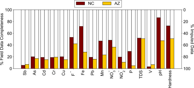
Data completeness percentage for groundwater parameters from the field data set for NC (maroon bars) and AZ (yellow bars). White bars (secondary y-axis) show the percentage of imputed data. Table S1 summarizes the specific values.
3.2. Data Imputation and Validation
3.2.1. Imputation Statistics
In addition to the limited completeness of our data sets (Figure 1), there was also variability in the combination (i.e., co-occurrence) of parameters measured. Consequently, data imputation techniques could take advantage of the existing co-occurring data sets with little concern for sampling bias. Figure 1 summarizes the imputation percentage for each of the water quality parameters; Table S1 summarizes the exact numbers of data points. For AZ, there were 13,363 field sampling locations with 91,765 total chemical measurements, rising to 401,760 chemical values after data imputation. For NC, there were 2,948 field sampling locations with 20,924 total chemical measurements, rising to 52,845 values after data imputation. Antimony required the most imputation, with 94% of its values imputed in the NC data set and 93% in the AZ data set. Conversely, pH had the lowest imputation percentage in NC (13%), while fluoride had the lowest imputation percentage in AZ (58%). The sparser data set for AZ resulted in a higher proportion of its values being imputed.
3.2.2. Distribution Comparison with Field Data Set
To evaluate the plausibility of the imputed data, we employed a combination of graphical and numerical assessments. Figure 2 compares the values for each water quality parameter between the original field (incomplete) data set with the corresponding values imputed by AMELIA; Figure S6 shows the companion plot for MICE. In Figure 2 we see that the median values from the field data and those imputed were comparable, both often falling within the same order of magnitude. For example, with arsenic, the field data and imputed values were equivalent (9.0 ppb) in AZ and very similar in NC (4.5 versus 3.2 ppb, respectively). Despite discrepancies in nitrate, 26 mgNO3-N/L in the field data versus 16 mgNO3–N/L in the imputed values for AZ, and 6.7 mgNO3-N/L versus 7.4 mgNO3-N/L for NC, imputed values remain significant because they are below the USEPA’s MCL of 10 mgNO3-N/L, demonstrating the imputed data’s accuracy and environmental relevance. Furthermore, to evaluate the imputation performance of AMELIA for “extremely sparse” sample sizes (i.e., data sets with >90% missing data for Sb or V, as shown in Figure 1), we included diagnostic test32 results in the Supporting Information (Figures S9 and S10).
Figure 2.
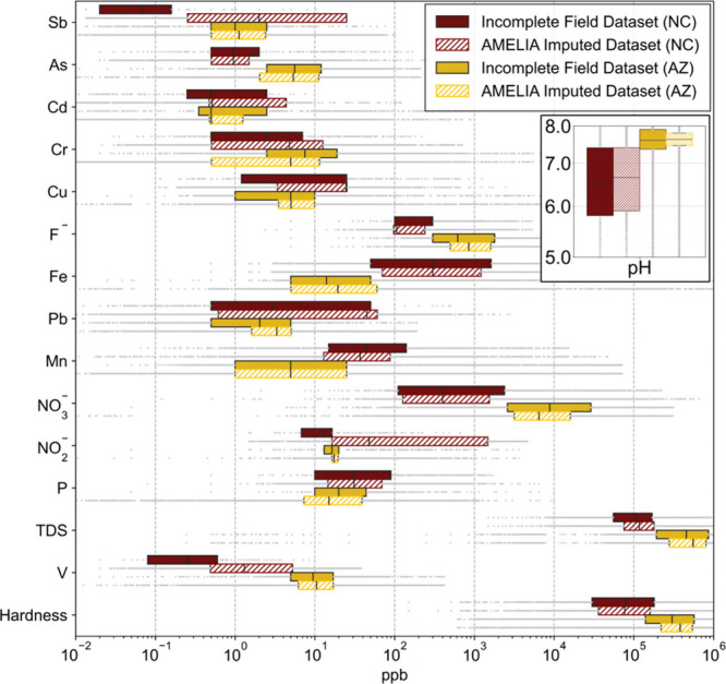
Distribution and variability between incomplete field data and AMELIA imputed data set. Solid bars represent data from measurements of field samples, while hashed-filled bars represent imputed data sets. The bar and whisker plot shows median values with a vertical line within the bar; ends of the bar represent 25th and 75th percentiles, and gray data points are outside those percentiles. Companion plots for MICE are provided as Figure S4.
To assess and compare the imputation results of AMELIA and MICE (Figures 2 and S4), the error was computed by subtracting the median of the historic data from the median of the imputed data for each parameter in each state (Table S2). Overall, when applied to our historic groundwater database, AMELIA demonstrated lower average and maximum errors than MICE. We used the Kolmogorov–Smirnov (KS) test to evaluate whether the distribution of 10 iterations of imputed data sets varies significantly. Here, the two-sample KS-distance method was used to check if the 10 iterations in the imputation process were producing significantly different variances in the imputed data set. We calculated the KS test statistics using the paired combination of 10 imputed data sets, resulting in a total of 10C2 = 45 pairwise KS-distance values for each groundwater parameter.33Figure 3 shows the mean and standard deviation of KS statistics for both states and imputation methods.
Figure 3.

Mean and confidence intervals of Kolmogorov–Smirnov distances of 16 parameters (Table S1) from the NC and AZ data sets after performing 10 imputations using the AMELIA (left) and MICE (right) methods.
Notably, both the AMELIA and MICE models faced difficulties when imputing vanadium in North Carolina due to multicollinearity and a high percentage of missingness. However, the AMELIA-imputed data sets consistently showed lower KS distances for all 16 parameters, regardless of the original field data being absent in Arizona. The differences in confidence levels between AMELIA and MICE were attributed to algorithmic variations and the level of missing data. AMELIA uses a multivariable data distribution,21 whereas MICE imputes using a one-by-one basis.20 A smaller KS-distance value signifies that the underlying distribution of a parameter in all 10 data sets is consistent, indicating low uncertainty in the imputed data. Additionally, the confidence intervals indicated some variation between the imputed 10 data sets. In the AZ data set, AMELIA showed a slightly lower average KS distance for the imputed parameters compared to MICE. These values remained within a 10% significance level. The lower KS distances observed with AMELIA could suggest overconfidence in its imputations. However, they could also indicate that AMELIA has an enhanced capacity to more accurately capture the distribution of missing data in specific data sets with a high volume of training data points. Additionally, parameters with a greater number of missing values tend to exhibit a higher mean KS-distance and larger confidence intervals (Figure 3), indicating that the algorithm has a higher uncertainty in cases with fewer available data points. While the lower KS-distances observed with MICE might suggest an overconfidence in its imputations, they could alternatively indicate MICE’s enhanced capacity to more accurately capture the distribution of missing data in our specific data set.
The imputed parameters obtained from both AMELIA and MICE showed accuracy within the 5% to 10% significance level for the computed KS distance. Notably, the lower KS distances observed with AMELIA may indicate potential overconfidence in the imputed data sets, possibly influenced by the high volume of data points in Arizona. Overall, the multiple imputed data sets by AMELIA suggested reasonable confidence in the generated data sets, while MICE showed slight overestimations based on the boxplot distribution.
3.3. Co-occurrence and Geospatial Occurrence of Groundwater Pollutants of Health Concern
Imputed data aid in understanding the probable distribution of chemicals in water (Figure 2) plus their co-occurrence and potential geospatial hot-spots. Sparse data for various health-related chemicals in each field sample necessitated data imputation to uncover potential co-occurrences, offering valuable insights for targeted field sampling to validate and mitigate associated risks. Figure 4 shows the percentage of sampling sites exceeding the health-based concentration of concern for individual chemicals, based both on sparse field data and after data imputation. The field data set indicated that 75% to 80% of field sampling locations had no co-occurrence with pollutants that exceeded their respective MCLs. Antimony, arsenic, cadmium, chromium, copper, and lead were the most common metals exceeding health-based levels in both field and imputed data sets. However, interpretation of AMELIA and MICE imputed values suggests that only 15% to 55% of sampling locations may have no health risks (i.e., zero samples above health-based limits). Imputed data suggested more frequent co-occurrence of regulated pollutants. Specifically, in all cases, imputed data reveal 2 to 5 times greater number of sampling locations with a predicted potential to surpass health-based limits, ranging from 1 to 6 co-occurring chemicals above health-based levels, as represented on the x-axis scale in Figure 4.
Figure 4.

Number of co-occurring chemicals and their percentage of groundwater sample locations that exceed the health based limits for the pollutants listed in Table 1.
Figure 4 illustrates the frequency of co-occurrence using field data alone compared to the improvements in risk identification through data imputation. The field data summarized in Figure 4 revealed that approximately three-quarters of the samples exhibited no chemicals above the threshold of potential health concern. Moreover, the likelihood of observing multiple (n ≥ 2) co-occurring chemicals above potential health concern levels was higher in Arizona than in North Carolina. Individual parameter correlation matrices were developed (Figures S7 and S8). While a few chemicals showed modest correlations (r > 0.5), the lack of exact 1:1 chemical correlation supported the need for the fingerprinting machine learning for both AMELIA and MICE. Overall, using data imputation techniques on sparse field data (Figure 1) provided a more comprehensive understanding of potential health risks associated with groundwater (Figure 4). This enhanced understanding is crucial, particularly when considering emerging approaches that consider antagonistic health effects from mixtures of pollutants.12
Imputed data maintained geospatial locational information. Maps for Arizona and North Carolina in Figures S9 and S10 depict field and imputed data for various inorganic chemicals. Each map highlights areas of the states where missing field data exist. For example, Figure S9a and S10a show where the 10% of field samples (from Figure 1) that have measured antimony concentrations are geospatially located along with locations of the additional 90% of the sites with imputed antimony values. Approximately 25% of the imputed data were above the MCL of 0.006 mg/L for antimony, and Figures S9a and S10a geospatially locate these hotspots. Antimony does not seem to co-occur with arsenic, but instead with Cd, Cu, or Pb (Figure S7). Overall, imputed occurrence data could provide insights and aid in strategically allocating potentially limited financial resources to collect and measure pollutant concentrations in additional field samples in regions with sparse data availability within the states.
Data imputation should be considered only as the first step in identifying occurrence hotspots. For example, over 90% of the antimony occurrence data needed to be imputed (Figure 1). Figure 2 shows that the imputed antimony data were an order of magnitude greater than the field data in NC, although field and imputed antimony concentrations had similar median and 25th to 75th percentile distributions in AZ, but much higher outliers beyond these distributions. Several factors may contribute to the overprediction in NC, most notably a much smaller number of samples in NC (339) versus AZ (2,918). To quantitatively assess the deviation or biases present in certain parameters within the comprehensive water quality matrix, the Mean Absolute Error (MAE) was calculated (Table S2). Data imputation in such cases should be viewed as useful identification of potential hotspots of elevated pollutant concentrations. Subsequently, as a second step, a state, city, or other agency can use data imputation to strategically prioritize locations and allocate financial resources for future sampling and analyses. As a final step, data from the informed field sampling campaigns can then be used to repeat the imputation process, reducing uncertainty in the distribution of imputed pollutant concentrations. Similar iterative approaches to prioritize sampling and refine data imputation would be worthwhile for other parameters with high levels of data imputation and/or when occurrence distributions differ significantly between field and imputed concentrations (e.g., Mn, NO3–, V).
Data imputation techniques provide valuable insights into water quality issues, but limitations must be acknowledged. The AMELIA and MICE methods can be challenged in predicting extreme values or infrequent events in sparse data sets. AMELIA’s assumption of a Gaussian distribution may overlook complex patterns in real-world data, leading to the loss of crucial information. The Kolmogorov–Smirnov (KS) distance used only addresses variances among imputed data set pairs, without calculating bias that would require real-world data for comprehensive assessment. Our approach of setting nondetects as half of the detection limit values, despite implemented training data constraints, may have introduced high extreme values. Furthermore, the evaluation of model performance based on interquartile range visualization and standard error calculation may not be a sufficiently robust predictor without validation against real-world data. Using the Kolmogorov–Smirnov (KS) distance addresses variances but not bias, and setting nondetects to half the detection limit may introduce high extreme values. Model performance evaluations based on interquartile ranges and standard errors lack robustness without real-world validation.
3.4. Water Treatment Implications
Water chemistry plays a significant role in determining and assessing the appropriate technologies for treating water pollutants that are of health concerns. Some nonregulated water chemistry parameters, even those with minimal health risks (Table 1), can profoundly impact the technical and economic aspects of treating health-related pollutants. To illustrate this impact, we provide a few examples related to the treatment of arsenic, nitrate, or hardness.
The co-occurrence of arsenic with iron in water significantly influences the treatment process selection from technologies such as packed-bed adsorption, oxidation-filtration, or coagulation-filtration. Each quadrant in Figure 5 represents a different treatment process. Iron concentrations are relevant because to remove arsenic in coagulation-filtration processes requires sufficient iron be present to exceed its solubility and facilitate precipitation of iron hydroxide floc that adsorbs arsenate.34 As annotated in Figure 5a, Quadrant I samples do not require arsenic treatment to meet the current drinking water regulation (i.e., arsenic concentration is below 10 μg/L MCL). Quadrant II samples have high arsenic concentrations and low iron concentrations, so using ambient iron in the water to produce floc (usually after oxidation with chlorine) would be insufficient to reduce treated water arsenic below the MCL. Therefore, packed bed adsorption or ion exchange would be the targeted treatment process.35,36 Quadrant III samples have co-occurring arsenic with elevated iron sufficient to remove arsenic to below the MCL. Quadrant IV samples have some iron but would require additional iron coagulant to form sufficient floc surfaces to remove arsenic from treated water.
Figure 5.

Treatability of groundwater samples with adsorption and chemical precipitation. (a) All field data points plotted in four treatment category quadrants (I, II, III, IV), (b) AMELIA imputed data points that have silica >20 ppm, (c) AMELIA imputed points that do not fall under any of the following criteria (silica >20 ppm and phosphate > arsenic, vanadium > arsenic, vanadium plus phosphate > arsenic), (d) AMELIA imputed data points having phosphate > arsenic, (e) AMELIA imputed data points where vanadium > arsenic, (f) AMELIA imputed data points that have vanadium plus phosphate > arsenic concentrations.
We focus our discussion on arsenic occurrence data for AZ (yellow symbols in Figure 5) because NC had far fewer samples with arsenic above the MCL (maroon symbols). Table 2 summarizes the percentage distribution and total number of samples within each “treatment” related quadrant. Figure 5a considers only the sparse field sampling data, whereas Figure 5b–f include data after AMELIA imputation. Whereas 74% of the field samples were below the arsenic MCL (quadrant I), the imputed data set revealed more potential samples likely to exceed 10 μg/L (i.e., only 57% below the MCL). Most of the newly identified samples fell into quadrant II, which indicated fairly low iron levels and would consequently require adsorbent-based arsenic treatment systems.
Table 2. Water Treatability Statistics Are Associated with Figure 5a.
| arsenic treatment quadrant associated with co-occurrence
of iron (from Figure 5) |
||||||
|---|---|---|---|---|---|---|
| co-occurrence scenario | data source | I | II | III | IV | total # samples |
| All Data | Field AZ | 74% | 24% | 1% | 1% | 5,405 |
| Imputed AZ | 57% | 38% | 3% | 1% | 26,784 | |
| Field NC | 86% | 3% | 10% | 0% | 1,167 | |
| Imputed NC | 95% | 1% | 4% | 0% | 3,523 | |
| Si > 20 ppm | Imputed AZ | 55% | 40% | 4% | 1% | 24,713 |
| Imputed NC | 89% | 2% | 8% | 0% | 1,291 | |
| P > As | Imputed AZ | 61% | 35% | 4% | 1% | 24,816 |
| Imputed NC | 95% | 1% | 4% | 0% | 3,495 | |
| V > As | Imputed AZ | 66% | 30% | 3% | 1% | 20,899 |
| Imputed NC | 95% | 1% | 4% | 0% | 2,012 | |
| P > As | Imputed AZ | 68% | 28% | 3% | 0% | 20,070 |
| and V > As | Imputed NC | 95% | 1% | 4% | 0% | 2,009 |
Values under each column show the number of groundwater samples in each water treatment method. Only field and AMELIA imputed data are shown below.
Silica adsorbs to iron-based adsorbents commonly used for arsenic treatment, and 40% of the imputed data co-occurs with silica above 20 ppm (Figure 5b)—levels that would result in significant fouling and shorten the expected operational life of iron packed bed adsorbent treatment processes. The similar chemical structure of vanadate and phosphate compared with arsenate results in competition for adsorption sites on metal (hydr)oxide adsorbents or flocs, thus decreasing the effectiveness of these arsenic treatment technologies. Competition for co-occurring oxoanions was considered to occur when their molar concentrations exceeded the molar concentration of arsenic. Figure 5c shows that very few samples had low co-occurrence of competing species. Imputed data revealed that phosphate (Figure 5d) and vanadate (Figure 5e) co-occurred with arsenic in 30% to 35% of the samples in quadrant II (Table 2), where adsorbent-based packed bed arsenic treatment technologies would likely be used. Figure 5f illustrates samples where the co-occurring molar concentrations of phosphate plus vanadate exceeded the arsenic concentration present in the water and would again exert competition for adsorbent binding sites. While most of the samples contained arsenic below the current MCL of 10 μg/L, it is noteworthy that this MCL was based on analytical detection capabilities in the year 2001 and is associated with a much lower excess cancer health-based limit of 1:10,000 rather than the typical 1:1,000,000 applied for most carcinogens. Trends illustrated in Figure 5b–f illustrate the potential for co-occurrence of nonregulated inorganic chemicals (silica, phosphate, vanadate) to have significant adverse impacts on arsenic removal should a lower MCL be promulgated or for homeowners installing point of use (POU) arsenic treatment systems.
Ion exchange water treatment is commonly applied to remove nitrate from water. However, other anions present in water (SO42–, Cl–, and HCO3–) increase treatment costs because they compete for resin exchange sites as nitrate ions (NO3–). Evaluating this competition requires comparing equivalent charge (mequiv/L) rather than mass (mgNO3-N/L) or molar concentrations. Figure 6 shows the sparse field and imputed data for nitrate co-occurrence with competing anions—shown as the sum of their equivalent concentrations. AZ has many more samples than NC where nitrate exceeded the MCL of 10 mgNO3-N/L, as well as having at least an order of magnitude higher level (mequiv/L) of competing anions. Contrasting Figure 6a versus b for Arizona clearly revealed the benefits of using data imputation to fill-in sparse co-occurrence data for competing anions. The imputed data (Figure 6b) showed much higher cumulative concentrations of co-occurring competing anions than the field data (Figure 6a). The concentrations of co-occurring anions are >10 times higher than nitrate and thus would significantly increase the frequency of ion exchange regeneration—which would consume more regenerant salts and increase brine disposal costs. It is noteworthy that emerging health effects studies show that lowering the nitrate MCL from 10 to 5 mgNO3-N/L may be appropriate to reduce unwanted cancer risks.5,37,38 Imputed data not only improved assessment for potential impacts of lowering nitrate regulatory limits but also, by considering the co-occurrence of competing anions, informs potential treatment costs associated with regulatory changes.
Figure 6.
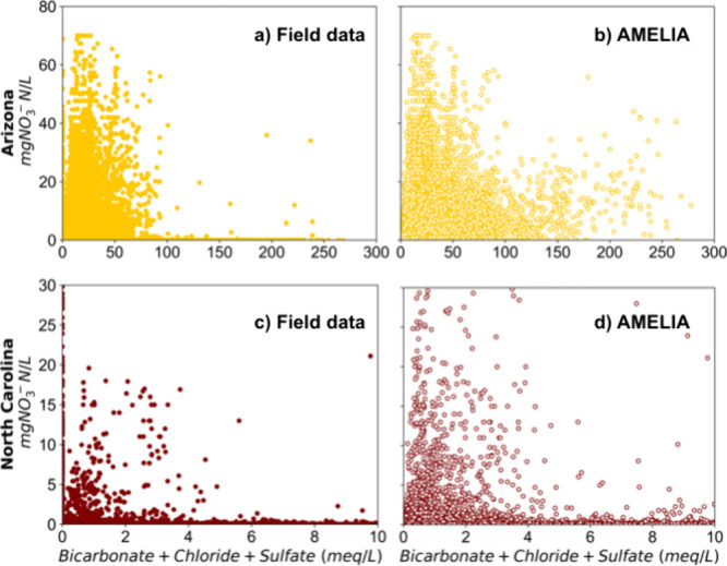
Co-occurrence of nitrate and competing inorganic ions associated with ion exchange treatment. The nitrate MCL is 10 mgNO3-N/L. Nitrate concentrations (mgNO3-N/L) can be converted to milli-equivalents per liter (meq/L) by dividing by 14 mequiv/mgNO3-N. Treatability corresponds to bicarbonate + sulfate + chloride concentration based on the field and imputed data set.
Hardness is one of the major reasons homeowners install POU water treatment devices because the presence of calcium and magnesium, which comprise hardness, causes aesthetic issues (taste, detergent/soap foaming) and scale-formation that impacts the lifespan of heating and plumbing devices. Hardness is a component of total dissolved solids (TDS), which is also noticeable to consumers in drinking water (Table 1). Roughly half of the field samples reported hardness or TDS (Figure 1). Imputed data for TDS and hardness have median concentrations comparable to those of field samples (Figure 2). Tables S4 and S5 summarize these ranges using terminology that consumers often understand (e.g., hard versus soft water). Identifying locations with higher hardness and TDS may allow communities and regulators to better understand public perceptions regarding their drinking water, how or if the public may be installing POU systems to address these aesthetic issues, and the potential where more centralized treatment could have significant benefits for communities.
4. Environmental Implications
Groundwater quality data for the United States were downloaded from the Water Quality Data Portal and preprocessed to analyze the co-occurrence of important inorganic pollutants of health concern and chemicals that impact the removal of the pollutants by different treatment processes. These data sets were often collected for differing reasons, over decades, and did not always measure all the sample chemical parameters. These sampling discrepancies resulted in sparse data sets where identifying co-occurrence of chemicals was hampered by incomplete data sets. Here, the approach of using multiple imputation techniques is proposed to inform this prioritization process rather than replace the need for real-world data. We were able to show how data imputation using two different techniques (AMELIA and MICE) made the data sets more complete (Figure 1). Imputed data had median concentrations comparable to those of the field data (Figure 2) for most chemicals. While differences existed between the two machine learning techniques (Figure 3), both enabled interpretation of critical insights after the sparse incomplete fields in the data set were addressed.
Imputed data provided a better understanding of the potential number of water sources that potentially had one or more regulated pollutants present above the regulatory levels (Figure 4). The field data set indicated that 75% to 80% of field sampling locations had no co-occurrence with pollutants that exceeded their respective MCLs. However, interpretation of AMELIA and MICE imputed values suggests that only 15% to 55% of sampling locations may have no health risks (i.e., zero samples above health-based limits). Imputed data suggested more frequent co-occurrence of regulated pollutants.
Transitioning to less-sparse data sets presents significant opportunities to mitigate people’s exposure to chemicals of concern in drinking water sources. First, by applying data imputation to specific sampling locations, the imputed data become geospatially available, enabling the identification of regions where drinking water may pose higher risks (Figures S9 and S10). This approach allows for the targeted deployment of limited field sampling resources to collect and analyze new samples from these potentially “high-risk” locations.
Second, new hazard and exposure analyses or advancements in chemical detection sensitivity occasionally warrant justification for reducing MCLs. For instance, the arsenic MCL was lowered from 50 to 10 μg/L in 2001. Emerging evidence suggests that reducing the nitrate MCL from 10 to <5 mgNO3-N/L could mitigate adverse health outcomes. Machine learning can aid regulatory determinations by assessing the likely impact of such changes because imputed data provide concentration data, not solely compliance or lack thereof with existing MCLs.
Third, treatment process selection and costs are crucial aspects of any new drinking water regulatory determination. Machine learning mitigates the sparsity of nonregulated chemical concentrations, which often co-occur with pollutants exceeding MCLs, thus offering a broader data set to estimate treatment methods and associated costs for compliance with drinking water regulations. Moreover, including nonregulatory chemical concentrations provides a basis for offering grant funding to help municipalities construct water treatment infrastructure. Less sparse data sets, particularly in rural communities that rely on private wells, can help identify regions where POU in-home treatment devices could significantly reduce exposure risks to chemical pollutants.
The proposed four-step iterative approach has the potential to reduce uncertainty and provide a framework for prioritizing sampling locations and chemical parameters for state agencies with limited financial resources, making it nearly impossible to sample all groundwater, all of the time, for all chemicals. First, performing machine learning on existing water quality data helps identify potential “hot spots” for prioritizing future sampling campaigns to collect additional groundwater chemistry data. State agencies will also consider other factors in prioritizing future sampling efforts, such as populations potentially exposed to chemicals in groundwater, local industrial activities, and regulatory requirements. Second, collecting new groundwater chemistry data enhances the completeness of data sets. Third, updated data sets can be used to validate machine learning predictions. Fourth, providing less sparse data sets helps improve data imputation. This approach holds significant promise in advancing efforts targeted at the in situ remediation of both geogenic and anthropogenic groundwater contamination.
By utilizing data imputation to identify the entire water matrix associated with the co-occurrence of elevated pollutant levels, the imputed water chemistry can potentially “fingerprint” common geological sources (e.g., arsenic from shale formations) or common land uses (e.g., nitrate co-occurrence with high TDS may indicate evaporated water used for agricultural irrigation). Similarly, the co-occurrence of lower pH and high copper can indicate acid-mine drainage impacting groundwater in regions like Arizona. Data imputation is especially valuable in data-sparse sampling scenarios, such as when samples are collected from household wells or under-resourced communities. In fact, a key motivation for this work was to identify poor water quality used as drinking water in colonias along the US-Mexico border, where many of these unincorporated communities are not part of public drinking water systems, and limited water quality data sets exist to identify where water was withdrawn or hauled.39−42 This review explores only a few of the occurrence and treatment insights gained through the evaluation of imputed data, and future work will delve into additional environmental impacts.
There were notable disparities in the number of chemical analyses conducted and the completeness of databases and concentrations of inorganic chemicals between the two states examined (AZ and NC). Despite these data input limitations, we successfully applied the same workflow and data imputation approaches to mitigate the sparse nature of the data sets. In the future, based on the success observed in these two states, we plan to extend this machine learning approach to all states. We aim to leverage the findings to gain a deeper understanding of the co-occurrence of inorganic chemicals in groundwaters used as municipal public drinking water or private-home water supplies.
Beyond the benefits stated above for state regulatory agencies, future research could prioritize field validation in areas with high data gaps and potential hotspots. Enhancing imputation algorithms to handle extreme values and integrating additional data sources, such as geological or land use information, could improve accuracy. Expanding these methods across diverse regions would help to assess generalizability and identify region-specific challenges. Emphasizing high-missing-parameter sampling and interdisciplinary collaboration will be essential for refining models and enhancing their reliability, ultimately informing better environmental management and policy decisions.
Acknowledgments
This work was supported by the Science and Technologies for Phosphorus Sustainability (STEPS) Center, a National Science Foundation Science and Technology Center (CBET-2019435), and The National Institute of Environmental Health Sciences through the Metals and metal mixtures: Cognitive aging, remediation, and exposure sources (MEMCARE) center (#P42ES030990). We acknowledge discussions with state regulatory agencies in Arizona regarding, in the face of limited financial resources for monitoring, the importance of reducing the uncertainty and prioritizing locations for groundwater sampling and analysis. Laurel Passantino provided technical editing.
Supporting Information Available
The Supporting Information is available free of charge at https://pubs.acs.org/doi/10.1021/acs.est.4c05203.
Additional experimental details, materials, and methods, including list of water quality parameters, data limitation, and curation process, descriptive statistics, correlation test details, geospatial maps of incomplete and imputed data (PDF)
Author Contributions
# A.U.M., M.I., and A.V.G. contributed equally to this paper.
The authors declare no competing financial interest.
Supplementary Material
References
- Belitz K.; Fram M. S.; Lindsey B. D.; Stackelberg P. E.; Bexfield L. M.; Johnson T. D.; Jurgens B. C.; Kingsbury J. A.; McMahon P. B.; Dubrovsky N. M. Quality of Groundwater Used for Public Supply in the Continental United States: A Comprehensive Assessment. ACS ES&T Water 2022, 2 (12), 2645–2656. 10.1021/acsestwater.2c00390. [DOI] [Google Scholar]
- Lapworth D. J.; Boving T. B.; Kreamer D. K.; Kebede S.; Smedley P. L. Groundwater quality: Global threats, opportunities and realising the potential of groundwater. Science of The Total Environment 2022, 811, 152471. 10.1016/j.scitotenv.2021.152471. [DOI] [PubMed] [Google Scholar]
- Misstear B.; Vargas C. R.; Lapworth D.; Ouedraogo I.; Podgorski J. A global perspective on assessing groundwater quality. Hydrogeology Journal 2023, 31 (1), 11–14. 10.1007/s10040-022-02461-0. [DOI] [Google Scholar]
- Thorslund J.; van Vliet M. T. H. A global dataset of surface water and groundwater salinity measurements from 1980–2019. Scientific Data 2020, 7 (1), 231. 10.1038/s41597-020-0562-z. [DOI] [PMC free article] [PubMed] [Google Scholar]
- Ward M. H.; Jones R. R.; Brender J. D.; de Kok T. M.; Weyer P. J.; Nolan B. T.; Villanueva C. M.; van Breda S. G. Drinking Water Nitrate and Human Health: An Updated Review. International Journal of Environmental Research and Public Health 2018, 15 (7), 1557. 10.3390/ijerph15071557. [DOI] [PMC free article] [PubMed] [Google Scholar]
- Coyte R. M.; Vengosh A. Factors Controlling the Risks of Co-occurrence of the Redox-Sensitive Elements of Arsenic, Chromium, Vanadium, and Uranium in Groundwater from the Eastern United States. Environ. Sci. Technol. 2020, 54 (7), 4367–4375. 10.1021/acs.est.9b06471. [DOI] [PubMed] [Google Scholar]
- Kumar M.; Goswami R.; Patel A. K.; Srivastava M.; Das N. Scenario, perspectives and mechanism of arsenic and fluoride Co-occurrence in the groundwater: A review. Chemosphere 2020, 249, 126126. 10.1016/j.chemosphere.2020.126126. [DOI] [PubMed] [Google Scholar]
- Allaire M.; Wu H.; Lall U. National trends in drinking water quality violations. Proc. Natl. Acad. Sci. U.S.A. 2018, 115 (9), 2078. 10.1073/pnas.1719805115. [DOI] [PMC free article] [PubMed] [Google Scholar]
- Smith A. H.; Steinmaus C. M. Health Effects of Arsenic and Chromium in Drinking Water: Recent Human Findings. Annual Review of Public Health 2009, 30, 107–122. 10.1146/annurev.publhealth.031308.100143. [DOI] [PMC free article] [PubMed] [Google Scholar]
- Gifford M.; Chester M.; Hristovski K.; Westerhoff P. Human health tradeoffs in wellhead drinking water treatment: Comparing exposure reduction to embedded life cycle risks. Water Res. 2018, 128, 246–254. 10.1016/j.watres.2017.10.014. [DOI] [PubMed] [Google Scholar]
- Sexton K.; Hattis D. Assessing Cumulative Health Risks from Exposure to Environmental Mixtures—Three Fundamental Questions. Environ. Health Perspect. 2007, 115 (5), 825–832. 10.1289/ehp.9333. [DOI] [PMC free article] [PubMed] [Google Scholar]
- Antonelli J.; Wilson A.; Coull B. A. Multiple exposure distributed lag models with variable selection. Biostatistics 2023, 25( (1), ), 1. 10.1093/biostatistics/kxac038. [DOI] [PMC free article] [PubMed] [Google Scholar]
- Hu X. C.; Dai M.; Sun J. M.; Sunderland E. M. The Utility of Machine Learning Models for Predicting Chemical Contaminants in Drinking Water: Promise, Challenges, and Opportunities. Current Environmental Health Reports 2023, 10 (1), 45–60. 10.1007/s40572-022-00389-x. [DOI] [PMC free article] [PubMed] [Google Scholar]
- Honaker J.; King G. What to Do about Missing Values in Time Series Cross Section Data. American Journal of Political Science 2010, 54, 561–581. 10.1111/j.1540-5907.2010.00447.x. [DOI] [Google Scholar]
- Horton N. J.; Kleinman K. P. Much Ado About Nothing. American Statistician 2007, 61 (1), 79–90. 10.1198/000313007X172556. [DOI] [PMC free article] [PubMed] [Google Scholar]
- Adhikari D.; Jiang W.; Zhan J.; He Z.; Rawat D. B.; Aickelin U.; Khorshidi H. A. A Comprehensive Survey on Imputation of Missing Data in Internet of Things. ACM Comput. Surv. 2023, 55 (7), 133. 10.1145/3533381. [DOI] [Google Scholar]
- Lombard M. A.; Bryan M. S.; Jones D. K.; Bulka C.; Bradley P. M.; Backer L. C.; Focazio M. J.; Silverman D. T.; Toccalino P.; Argos M.; Gribble M. O.; Ayotte J. D. Machine Learning Models of Arsenic in Private Wells Throughout the Conterminous United States As a Tool for Exposure Assessment in Human Health Studies. Environ. Sci. Technol. 2021, 55 (8), 5012–5023. 10.1021/acs.est.0c05239. [DOI] [PMC free article] [PubMed] [Google Scholar]
- Ayotte J. D.; Medalie L.; Qi S. L.; Backer L. C.; Nolan B. T. Estimating the High-Arsenic Domestic-Well Population in the Conterminous United States. Environ. Sci. Technol. 2017, 51 (21), 12443–12454. 10.1021/acs.est.7b02881. [DOI] [PMC free article] [PubMed] [Google Scholar]
- Betrie G. D.; Sadiq R.; Tesfamariam S.; Morin K. A. On the Issue of Incomplete and Missing Water-Quality Data in Mine Site Databases: Comparing Three Imputation Methods. Mine Water and the Environment 2016, 35 (1), 3–9. 10.1007/s10230-014-0322-4. [DOI] [Google Scholar]
- Kabir G.; Tesfamariam S.; Hemsing J.; Sadiq R. Handling incomplete and missing data in water network database using imputation methods. Sustainable and Resilient Infrastructure 2020, 5 (6), 365–377. 10.1080/23789689.2019.1600960. [DOI] [Google Scholar]
- Honaker J.; King G.; Blackwell M. Amelia II: A Program for Missing Data. Journal of Statistical Software 2011, 45 (7), 1–47. 10.18637/jss.v045.i07. [DOI] [Google Scholar]
- van Buuren S.; Groothuis-Oudshoorn K. mice: Multivariate Imputation by Chained Equations in R. Journal of Statistical Software 2011, 45 (3), 1–67. 10.18637/jss.v045.i03. [DOI] [Google Scholar]
- Kim W., Cho W.; Choi J.; Kim J.; Park C.; Choo J.. A Comparison of the Effects of Data Imputation Methods on Model Performance. In 2019 21st International Conference on Advanced Communication Technology (ICACT), 2019. [Google Scholar]
- Pampaka M.; Hutcheson G.; Williams J. Handling missing data: analysis of a challenging data set using multiple imputation. International Journal of Research & Method in Education 2016, 39 (1), 19–37. 10.1080/1743727X.2014.979146. [DOI] [Google Scholar]
- Rahm E.; Do H. Data Cleaning: Problems and Current Approaches. IEEE Data Eng. Bull. 2000, 23, 3–13. [Google Scholar]
- Zhong S.; Zhang K.; Bagheri M.; Burken J. G.; Gu A.; Li B.; Ma X.; Marrone B. L.; Ren Z. J.; Schrier J.; Shi W.; Tan H.; Wang T.; Wang X.; Wong B. M.; Xiao X.; Yu X.; Zhu J.-J.; Zhang H. Machine Learning: New Ideas and Tools in Environmental Science and Engineering. Environ. Sci. Technol. 2021, 55 (19), 12741–12754. 10.1021/acs.est.1c01339. [DOI] [PubMed] [Google Scholar]
- NWQMC . Water Quality Portal - National Water Quality Monitoring Council. 2023. [cited 2023 04/16]; Available from https://www.waterqualitydata.us/#mimeType=csv&providers=NWIS&providers=STEWARDS&providers=STORET.
- Richards L. E. Journal of Marketing Research 1989, 26 (3), 374–375. 10.1177/002224378902600317. [DOI] [Google Scholar]
- van Buuren S.Flexible Imputation of Missing Data, 1st ed.; Chapman and Hall/CRC, New York, NY, 2012; p 342. [Google Scholar]
- Pedregosa F.; Varoquaux G.; Gramfort A.; Michel V.; Thirion B.; Grisel O.; Blondel M.; Prettenhofer P.; Weiss R.; Dubourg V. Scikit-learn: Machine learning in Python. Journal of Machine Learning Research 2011, 12, 2825–2830. [Google Scholar]
- Schröer G.; Trenkler D. Exact and randomization distributions of Kolmogorov-Smirnov tests two or three samples. Computational Statistics & Data Analysis 1995, 20 (2), 185–202. 10.1016/0167-9473(94)00040-P. [DOI] [Google Scholar]
- Abayomi K.; Gelman A.; Levy M. Diagnostics for multivariate imputations. Journal of the Royal Statistical Society, Series C: Applied Statistics 2008, 57, 273–291. 10.1111/j.1467-9876.2007.00613.x. [DOI] [Google Scholar]
- Nguyen C. D.; Carlin J. B.; Lee K. J. Diagnosing problems with imputation models using the Kolmogorov-Smirnov test: a simulation study. BMC Medical Research Methodology 2013, 13 (1), 144. 10.1186/1471-2288-13-144. [DOI] [PMC free article] [PubMed] [Google Scholar]
- Lytle D.; Sorg T. J.; Snoeyink V. L. Optimizing arsenic removal during iron removal: Theoretical and practical considerations. Journal of Water Supply: Research and Technology - AQUA 2005, 54, 545–560. 10.2166/aqua.2005.0048. [DOI] [Google Scholar]
- Sorg T.; Chen A. S. C.; Wang L.; Kolisz R. Regenerating an Arsenic Removal Iron-Based Adsorptive Media System, Part 1: The Regeneration Process. Journal American Water Works Association 2017, 109 (5), 13–24. 10.5942/jawwa.2017.109.0045. [DOI] [PMC free article] [PubMed] [Google Scholar]
- Sorg T. J.; Chen A. S. C.; Wang L.; Lytle D. A. Removing co-occurring contaminants of arsenic and vanadium with full-scale arsenic adsorptive media systems. AQUA - Water Infrastructure, Ecosystems and Society 2021, 70 (5), 665–673. 10.2166/aqua.2021.148. [DOI] [PMC free article] [PubMed] [Google Scholar]
- García Torres E.; Pérez Morales R.; González Zamora A.; Ríos Sánchez E.; Olivas Calderón E. H.; Alba Romero J.d.J.; Calleros Rincón E. Y. Consumption of water contaminated by nitrate and its deleterious effects on the human thyroid gland: a review and update. International Journal of Environmental Health Research 2022, 32 (5), 984–1001. 10.1080/09603123.2020.1815664. [DOI] [PubMed] [Google Scholar]
- Temkin A.; Evans S.; Manidis T.; Campbell C.; Naidenko O. V. Exposure-based assessment and economic valuation of adverse birth outcomes and cancer risk due to nitrate in United States drinking water. Environmental Research 2019, 176, 108442. 10.1016/j.envres.2019.04.009. [DOI] [PubMed] [Google Scholar]
- Wutich A.; Jepson W.; Velasco C.; Roque A.; Gu Z.; Hanemann M.; Hossain M. J.; Landes L.; Larson R.; Li W. W.; Morales-Pate O.; Patwoary N.; Porter S.; Tsai Y.-s.; Zheng M.; Westerhoff P. Water insecurity in the Global North: A review of experiences in U.S. colonias communities along the Mexico border. WIREs Water 2022, 9 (4), e1595. 10.1002/wat2.1595. [DOI] [Google Scholar]
- Gu Z.; Li W.; Hanemann M.; Tsai Y.; Wutich A.; Westerhoff P.; Landes L.; Roque A. D.; Zheng M.; Velasco C. A.; Porter S. Applying machine learning to understand water security and water access inequality in underserved colonia communities. Computers, Environment and Urban Systems 2023, 102, 101969. 10.1016/j.compenvurbsys.2023.101969. [DOI] [Google Scholar]
- Wutich A.; Thomson P.; Jepson W.; Stoler J.; Cooperman A. D.; Doss-Gollin J.; Jantrania A.; Mayer A.; Nelson-Nuñez J.; Walker W. S.; Westerhoff P. MAD water: Integrating modular, adaptive, and decentralized approaches for water security in the climate change era. WIREs Water 2023, 10 (6), e1680. 10.1002/wat2.1680. [DOI] [PMC free article] [PubMed] [Google Scholar]
- Thomson P.; Stoler J.; Wutich A.; Westerhoff P. MAD water (modular, adaptive, decentralized) systems: New approaches for overcoming challenges to global water security. Water Security 2024, 21, 100166. 10.1016/j.wasec.2024.100166. [DOI] [Google Scholar]
Associated Data
This section collects any data citations, data availability statements, or supplementary materials included in this article.