

Abstract
Differential evolution (DE) is a robust evolutionary algorithm for solving single-objective and multi-objective optimization problems (MOPs). While numerous multi-objective DE (MODE) variants exist, prior research has primarily focused on parameter control and mutation operators, often neglecting the issue of inadequate population distribution across the objective space. This paper proposes an external archive-guided radial-grid-driven differential evolution for multi-objective optimization (Ar-RGDEMO) to address these challenges. The proposed Ar-RGDEMO incorporates three key components: a novel mutation operator that integrates a radial-grid-driven strategy with a performance metric derived from Pareto front estimation, a truncation procedure that employs Pareto dominance in conjunction with a ranking strategy based on shifted similarity distances between candidate solutions, and an external archive that preserves elite individuals using a clustering approach. Experimental results on four sets of benchmark problems demonstrate that the proposed Ar-RGDEMO exhibits competitive or superior performance compared to seven state-of-the-art algorithms in the literature.
Subject terms: Engineering, Mathematics and computing
Introduction
In real-world scenarios, we frequently encounter the complexity of simultaneously optimizing multiple objectives, known as multi-objective optimization problems (MOPs)1. Researchers have shown significant interest in MOPs in recent years due to their relevance to diverse industrial applications2–5. These MOPs are prevalent in real-world applications, including vehicle path planning6, job shop scheduling7, feature selection8, neural network structure optimization9, and autonomous robotics services10. Unlike single-objective optimization problems (SOPs), MOPs pose the challenge of addressing multiple objectives that may conflict with each other simultaneously. The resolution of MOPs yields a set of Pareto optimal solutions, each representing a unique trade-off among objectives3. Inspired by biological processes such as reproduction, mutation, recombination, and selection, evolutionary algorithms (EAs) aim to effectively approximate solutions across various problem types without relying on assumptions about the underlying fitness landscape2.
Multi-Objective Evolutionary Algorithms (MOEAs) have gained widespread recognition as efficient methodologies for addressing MOPs. They handle MOPs with diverse characteristics and can generate the solution set in a single execution11,12. The effectiveness of MOEAs relies on two key factors: algorithm structure and employed search operators. Existing literature extensively categorizes algorithm structures into Pareto-based13,14, indicator-based15,16,17, and decomposition-based algorithms2–5. The algorithm’s structure plays a pivotal role in shaping its performance. Conversely, the selection of search operators in an MOEA significantly impacts its search effectiveness. Genetic algorithms (GA) are widely employed as search operators in most MOEAs. These operators are critical in shaping the algorithm’s capacity to explore the solution space efficiently.
Differential Evolution (DE) is renowned among evolutionary algorithms (EAs) for its simple yet robust search capabilities, which have proven effective in solving single-objective optimization problems (SOPs)18,19. Beyond this, researchers have successfully expanded DE’s scope to address MOPs with notable success. A key attribute of DE lies in its capacity to generate solutions characterized by significant diversity in their decision vectors, a critical facet for simultaneously exploring multiple non-dominated solutions in MOPs20. This unique feature underscores DE’s adaptability to handle the complexities inherent in MOPs. The accomplishments of DE in multi-objective optimization have encouraged the development of numerous variants known as MODE algorithms following its pioneering extension21. These MODE algorithms continue to push the boundaries of multi-objective optimization, building upon DE’s foundational principles while introducing innovative strategies to enhance performance and solution quality22.
As highlighted in22, DE faces two notable challenges in addressing MOPs. Initially, DE’s selection mechanism entails comparing every parent candidate solution with its respective trail vector. Nevertheless, this method proves ineffective in maintaining a diverse array of non-dominated individuals across the evolution process within MOP scenarios23. Secondly, the evolutionary process of DE frequently encounters stagnation and struggles with infrequent convergence due to its inherent high diversity. This issue is notably prominent in DE, reducing selection pressure towards the Pareto Front (PF) and producing a diverse solution set lacking thorough convergence24. Due to the increase in objectives, the convergence challenges of DE become even more pronounced for MOPs with numerous objectives, often referred to as many-objective optimization problems (MaOPs). This amplification further complicates the convergence process and hampers the effective application of DE in addressing MaOPs25.
Over the past few decades, several MODE approaches26–29 have emerged to tackle MOPs. Despite advancements, most established MODEs focus on refining adaptive strategies for mutation operators and control parameters to generate a higher-quality population from an initial one. However, they often overlook considerations regarding the distribution quality of this new population24. As far as we know, only a handful of studies22–24 in the current body of literature have emphasized enhancing the distribution quality of the population by leveraging feedback from the preceding search process. While significant advancements have been made, the development of MODEs for MOPs and MaOPs still faces considerable technical challenges. Firstly, although DE encounters convergence issues, the creation of mutation operators that effectively prioritize convergence remains inadequately addressed within MODEs. Secondly, despite efforts to devise self-adaptive strategies for MODEs, these approaches frequently overlook the quality of the target solutions30. Additionally, there exists a critical necessity for advancements to enhance the distribution quality of solutions within the MODE population24.
Our paper presents an innovative approach called external archive-guided radial-grid driven differential evolution for multi-objective optimization (Ar-RGDEMO) to address limitations. This method is designed to enhance convergence, coverage, and diversity, thereby significantly improving the effectiveness of solving complex MOPs. Ar-RGDEMO integrates a novel mutation operator, a ranking-based truncation approach, and an external archive guided by clustering. These techniques enhance the optimization process, improving its ability to address MOPs effectively.
The main contributions of this paper are summarized as follows:
Firstly, we have developed an innovative mutation operator that utilizes a radial-grid-driven strategy in conjunction with the performance indicator based on Pareto front estimation. The radial-grid-driven strategy aims to simultaneously preserve diversity while the performance indicator enhances convergence and coverage within the optimization process.
Next, a truncation procedure is implemented, utilizing a ranking approach that considers shifted similarity distances among candidate solutions, ensuring thorough evaluation based on their relative positions and enhancing truncation efficacy. Finally, an external archive is employed with a clustering approach to preserve elite individuals, ensuring their top-performing solutions persistently contribute to optimization.
We conducted thorough experimentation on 30 problems from four benchmark test suites to assess the proposed Ar-RGDEMO’s effectiveness compared to seven state-of-the-art algorithms. Our experimental findings demonstrate that the Ar-RGDEMO is superior to the seven benchmark algorithms.
The remainder of the paper is as follows. “Background” provides the research background and outlines the motivation behind our work. “Proposed method” offers a concise overview of the proposed approach, while “Empirical studies” delves into the presentation of experimental results and discussions. Finally, “Conclusions and future works” provides the concluding remarks for the paper.
Background
Related works
Although differential evolution is a relatively recent addition to the realm of EAs, it has consistently demonstrated exceptional search capabilities since its introduction by Storn and Price42. Further, the application of DE in tackling MOPs has shown significant promise. Researchers have made substantial progress investigating various aspects of DE, including adaptive strategies for mutation, parameter tuning, enhanced selection mechanisms, and methods for maintaining population diversity. Table 1 summarizes the literature on differential evolution for MOPs. The first adaptation of DE for MOPs was introduced in Pareto Differential Evolution (PDE)21. This approach generates a new population using DE operators and retains only the non-dominated solutions for subsequent iterations. An improved version for PDE, termed DEMO, is proposed in26 that incorporates fast nondominated sort and crowding distance for DE.
Table 1.
Summary of differential evolution algorithms for multi-objective optimization.
| Algorithm | Working principle |
|---|---|
| PDE21 | Generates new population using DE operators, retains only non-dominated solutions for subsequent iterations |
| DEMO26 | Incorporates fast non-dominated sort and crowding distance for DE |
| GDE327 | Hybrid approach combining elements from different selection schemes |
| MOSaDE31 | Dynamically selects suitable mutation strategies |
| OWMOSaDE29 | Adaptive selection of mutation strategies and independent crossover parameters for each objective |
| MODEA32 | Uses opposition learning-based population initialization and random localization based mutation operator |
| MODESA33 | Employs simulated annealing for candidate solution acceptance and prior life cycle concept |
| MyO-DEMR34 | Restricts difference vectors in DE for many-objective optimization |
| MOEAD-FRRMAB35 | Incorporates various DE operators with adaptive mutation operator rates |
| MOEAD-DYTS36 | Uses dynamic Thomson sampling-based adaptive operator selection |
| CMODE37 | Cooperative MODE with multiple populations, each addressing a single objective |
| AMPDE38 | Multi-population MODE with unique mutation strategies and intra-population competition |
| GAMODE22 | Employs grid indexes for parameter control, parent adaptation, and selection |
| DECOR30 | Reduces objectives by clustering Pareto front objectives and retaining centroid components |
| AMODE-RAVM24 | Utilizes evolutionary information to dynamically adjust control parameters |
| BiasMOSaDE23 | Introduces personal archives and biased mutation operators in MODE framework |
| MOEA/D39 | Decomposes MOP into scalar optimization subproblems and optimizes them simultaneously |
| MOEA/D-DE40 | Integrates DE operators into the MOEA/D framework |
| MOEA/D-PaS41 | Incorporates priority and satisfaction mechanism into MOEA/D |
In27, GDE3, an extension of generalized DE43, is proposed that adopts a hybrid approach, amalgamating elements from both selection schemes mentioned above, thus providing a nuanced and adaptable selection mechanism within MODE. In31, a self-adaptive MODE (MOSaDE) was proposed, which dynamically selects suitable mutation strategies. Expanding on this foundation, the authors from31 further refined their methodology by introducing objective-wise learning strategies MOSaDE (OWMOSaDE)29. This advancement facilitates the adaptive selection of mutation strategies and independent crossover parameters for each objective. In32, MODE with opposition learning-based population initialization and random localization-based mutation operator for MODE, termed MODEA, is proposed.
In33, a novel approach termed MODESA was proposed, where simulated annealing was proposed to control candidate solution acceptance during DE selection and the prior life cycle concept to avoid potential solutions stuck in the local optimum. In34, a strategy that restricts the difference vectors in DE was suggested to deal with many-objective optimization (MyO-DEMR). In addition, the inverted generational distance metric is coupled with Pareto dominance to preserve promising individuals for the later generation. In35, a variant of MOEA/D called MOEA/FRRMAB was introduced. This variant incorporates various differential evolution (DE) operators, with mutation operator rates adaptively determined through a multi-armed bandit scheme. Furthermore, an extension to the MOEA/DDYTS approach was suggested in36. This extension adopts a dynamic Thomson sampling-based adaptive operator selection method to choose operators based on performance.
In37, initial efforts were made towards a cooperative MODE (CMODE) with multiple populations, where each population addresses a single objective, facilitating a more comprehensive exploration of the solution space. Another iteration of a multi-population MODE was proposed in AMPDE38, where each subpopulation embraced its unique mutation strategy and competed for evolutionary resources, further enhancing diversity through intra-population competition. These diverse approaches collectively contribute to the robustness and effectiveness of diversity control mechanisms within MODE. In22, a novel grid-based MODE (GAMODE) was proposed that employs grid indexes for parameter control, parent adaptation, and parent selection. In30, a novel method termed DECOR was proposed that reduces objectives by clustering Pareto front objectives and retaining only centroid components of the most compact cluster, thus decreasing problem dimensionality.
In24, the authors have utilized the evolutionary information from solutions along each search direction to dynamically adjust control parameters in MODE (AMODE-RAVM), refining the adaptation process and enhancing efficiency. In23, a novel concept is presented (BiasMOSaDE) where a series of personal archives and a truncation procedure are introduced. These are seamlessly integrated into the MODE framework and complemented by the integration of multiple biased mutation operators. Moreover, numerous decomposition-based MOEAs in the literature have utilized the differential evolution (DE) operator to produce offspring solutions, including MOEA-D39, MOEAD-DE40, MOEAD-PaS41, among others.
Motivations
The literature demonstrates that the DE generation operation is commonly utilized as the offspring generation operator in MODEs, characterized by its distinctive mutation paradigms. Various implementations of DE mutations, such as “DE/rand/1,” “DE/rand/2,” “DE/best/1,” and “DE/current-to-best/1,” yield new trial solutions with diverse search behaviors. Although the “DE/rand/1” mutation, which randomly selects parents from the entire population, is prevalent, this simplistic approach often results in excessive diversity and convergence stagnation. Similarly, static parameter values are frequently employed for configuration, with only sporadic attempts at online adaptation. Additionally, only a few approaches choose alternative mutation forms, particularly those reliant on “best” solutions.
In MODE, leveraging suitable “best” solutions (hereafter denoted as ) can significantly enhance offspring generation. Nonetheless, defining and selecting such presents challenges. Two primary issues emerge:
Defining proves challenging in multiobjective scenarios, where the optimality of an MOP is characterized by a Pareto tradeoff solutions set.
should steer the population toward approximating the Pareto optimal set while exploring promising areas, effectively balancing convergence and diversity-both critical features for MODEs.
In the proposed mutation operator of Ar-RGDEMO, we effectively address the challenges outlined by integrating two pivotal components: the radial-grid-driven strategy and a performance metric based on Pareto front estimation. This formulation ensures robust identification of solutions, crucial for balancing convergence and diversity during optimization. The radial-grid-driven strategy systematically explores the solution space, enhancing coverage and search efficiency by partitioning it into distinct regions. This targeted exploration facilitates the discovery of promising solutions.
Moreover, the performance metric based on Pareto front estimation offers a quantitative assessment of solution quality, prioritizing solutions and achieving an optimal balance between conflicting objectives. Utilizing this metric identifies solutions that effectively converge while maintaining diversity, ensuring a well-distributed array across the Pareto front.
Proposed method
Framework of Ar-RGDEMO
Figure 1 depicts the flowchart of the proposed Ar-RGDEMO algorithm, which resembles conventional MODEs. A, which resembles conventional MODEs. Further, initially, a parent population, denoted as P, is formed by randomly generating N individuals. Subsequently, each population generation undergoes an evolutionary process where mutation and crossover operators are systematically applied to create a trial vector for every parent, facilitating exploration and exploitation of the solution space. The proposed Ar-RGDEMO introduces a novel radial-grid-based mutation operator to perturb each parent vector, enhancing the diversity of the population. Following this mutation step, binomial crossover and polynomial mutation operators refine the trial vectors, ensuring a comprehensive solution space exploration.
Fig. 1.

Flowchart of Proposed Ar-RGDEMO.
Next, the traditional one-to-one selection method of differential evolution is employed, leveraging the dominant relation between parent solutions, referred to as target vectors, and their corresponding trial vectors. If the trial vector outperforms the target vector, the target vector is replaced accordingly. Conversely, if the target vector outperforms the trial vector, the latter is disregarded. Both vectors are preserved in cases where neither vector demonstrates superiority. Subsequently, a truncation procedure is implemented using a ranking approach that considers the shifted distances between candidate solutions, refining the population by retaining only the most promising individuals. Finally, an external archive is maintained based on clustering to preserve the elite individuals, ensuring that valuable solutions are not lost throughout the optimization process, contributing to the algorithm’s robustness and effectiveness. This iterative procedure continues until the termination criteria are met, ensuring the algorithm converges towards high-quality solutions. A detailed explanation of the critical components of Ar-RGDEMO is presented in the subsequent sections, providing insights into its operation and effectiveness. Further, Algorithm 1 outlines the comprehensive framework of the proposed Ar-RGDEMO
Algorithm 1.
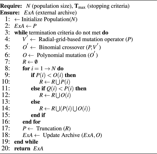
Overall procedure of Ar-RGDEMO
Radial grid-based mutation operator
The mutation operator in DE plays a pivotal role in population evolution as it is essential for exploring the search space and generating diverse solutions. Introducing variations to candidate solutions facilitates the discovery of promising regions in the solution space. Therefore, the effectiveness of the mutation operator significantly impacts the convergence speed and overall performance of the DE algorithm. This paper proposes a novel mutation operator to improve convergence speed and preserve population diversity simultaneously. In our proposed mutation operator, we incorporate the radial grid settings recommended in44, which specify the positions of individuals in the radial space. This integration of the radial grid into the mutation operator offers the advantage of preserving population diversity by evaluating the crowding condition of each solution.
Moreover, we utilize a performance indicator termed , based on Pareto front estimation, to ensure convergence and coverage. This indicator is a strategic guide, leveraging insights from Pareto front estimation to direct the optimization process toward convergence and coverage. By integrating radial grids with a performance indicator based on Pareto front estimation, our mutation operator effectively balances exploration and exploitation, facilitating robust optimization outcomes. The proposed mutation operator involves three steps: a) constructing a radial grid, b) evaluating the convergence indicator, and c) generating perturbed vectors. The main procedure of the radial-grid-based mutation operator is depicted in Algorithm 2.
Algorithm 2.

Radial grid-based mutation operator.
Constructing radial grid
The initial stage of the process involves establishing a radial grid within the objective space. This grid effectively partitions the space into discrete segments, facilitating structured organization and enhancing navigability. To improve the accuracy of the grid in assessing the crowding condition of individual solutions, it is advisable to ensure its adaptability to the evolving population. Essentially, the grid’s positioning should dynamically adjust in tandem with the evolution of the population. Therefore, we have developed an adaptive radial grid inspired by the approach proposed in44. Initially, the objective vectors of the current population undergo a normalization procedure, utilizing their ideal and nadir points derived from non-dominated solutions within the population.
Afterward, the normalized objective vectors undergo projection onto a two-dimensional radial space, transitioning from the initial high-dimensional objective space with the aid of projection weight vectors ( and ). The weight vectors are defined as follows:
| 1 |
| 2 |
Then, the boundaries of the projected solutions are identified to define the rectangular region containing these solutions. Next, this rectangular region is partitioned into uniform grids, where each side of the rectangle is divided into segments, with N representing the population size and M denoting the number of objectives. Lastly, the coordinates of each solution in radial space are computed, along with the grid label corresponding to its location within the divided rectangle.
Evaluating performance indicator
After establishing the radial grid, the subsequent step involves assessing a performance indicator based on estimating the Pareto front. This indicator quantitatively measures the algorithm’s proximity to achieving the optimal Pareto front and ensures coverage. Initially, to evaluate the performance indicator, the objective functions of each candidate solution are normalized. In multi-objective problems (MOPs), objectives may vary significantly in scale, resulting in specific objectives exerting a disproportionate influence on convergence and coverage measures within the objective space when normalization is neglected. Therefore, objective normalization is crucial for establishing a more robust and reliable convergence indicator to achieve convergence effectively. Each objective function , where , for a solution undergoes normalization in the following manner:
| 3 |
where and denotes the ideal point, while refers to the nadir point. Given that the Pareto Front (PF) remains elusive, the estimations of and often rely on the existing population. Every component of can be approximated as the minimum value of its corresponding objective discovered within the non-dominated individuals. Further, is evaluated using the M corner solutions as mentioned in45.
After normalization, the performance indicator () is mathematically defined as
| 4 |
where M is the number of objectives, is the objective function vector of individual x, P determines the shape of PF. To evaluate the P value, we have adopted the method proposed in45.
The process begins with computing the Lp-norm distances for all individuals to the origin point, denoted as , using various p-values. Following this computation, we determine the standard deviation , denoted as . A smaller value of indicates better consistency in the distribution of individuals concerning the LP-norm distance. Subsequently, we employ the contour curve obtained through the Lpminnorm method to approximate the shape of the Pareto front (PF), with corresponding to the smallest . We utilize the box plot46 to mitigate noise during PF shape estimation to identify outlier values in . Specifically, values surpassing are considered noise, where Q1 and Q3 represent the lower and upper quartiles of respectively, and is set to 1.5 as suggested in44. Before computing the standard deviation , we remove noise values from .
The performance indicator provides valuable insights into the algorithm’s performance and progression towards convergence by evaluating population diversity, solution quality, and convergence rate. This evaluation step is paramount in guiding the mutation process and ensuring the efficiency and effectiveness of the algorithm.
Generating perturbed vectors
In the final step of the mutation operator, perturbed vectors are generated based on insights gained from the radial grid and performance indicator evaluation. These vectors represent potential candidate solutions, introducing variability and diversity into the population. As highlighted in the motivations for this proposed approach, we utilize the “DE/current-to-best/1” mutation strategy in the mutation operator. This strategy generates perturbed vectors from each individual in the population (referred to as target solutions). The is effectively identified by leveraging information from the radial grid and performance indicator. Firstly, each target solution’s corresponding radial grid location is determined to facilitate perturbed vector generation. Subsequently, solutions within this radial grid location are identified. The solution with the least CVp among these solutions is considered the best. For a designated target solution , the perturbed vector is computed as:
| 5 |
where and are two randomly selected solutions from the existing population. By integrating these three steps, the mutation operator provides a systematic and informed approach to enhancing performance and efficiency, ultimately enabling more effective optimization in complex problem domains. Following the generation of perturbed vectors in the proposed Ar-RGDEMO approach, the process proceeds with applying binomial crossover22–24 and polynomial mutation47 techniques to these vectors. This step aims to generate offspring solutions by combining the parent solutions’ characteristics, further diversifying the population and exploring new regions of the solution space. Binomial crossover facilitates the exchange of genetic information between perturbed vectors, while polynomial mutation introduces small, random changes to individual components of the vectors. These combined processes contribute to exploring the solution space and discovering improved solutions in the evolutionary optimization process.
Algorithm 3.

Truncation procedure
Truncation procedure
After generating the offspring solutions, the traditional DE one-to-one selection method is employed, relying on the dominant relationship between parent solutions (referred to as target vectors) and their corresponding trial vectors. The solutions that survive this selection stage are copied into a set R and undergo a truncation procedure to preserve superior solutions, forming the parent population for subsequent generations. In Algorithm 3, the truncation procedure is described in detail. In the initial stage of the truncation procedure, individuals in set R undergo non-dominated sorting, categorizing them into distinct fronts based on dominance. For instance, consider individuals in R are categorized into various non-dominated fronts, denoted as . From these fronts, individuals from the top l rank levels are chosen to constitute a temporary population . The threshold l is determined as:
| 6 |
where N represents the size of population, P , and signifies the collection of individuals at rank level i.
Following this, a ranking procedure is implemented based on the shifted similarity distance between individuals. This method enhances the selection process by providing a more nuanced comparison between solutions in the objective space. Further, this mechanism effectively standardizes individual performance, enhancing comparative analysis in objective conflicts. The concept of shifted similarity distance was initially developed for many objective optimization problems, where traditional Pareto dominance-based approaches often struggle due to the high dimensionality of the objective space. However, recent studies48–50 have demonstrated the efficacy of shifted similarity distance in multi-objective optimization scenarios. Therefore, in the proposed Ar-RGDEMO, we have employed shifted similarity distance to evaluate candidate solutions effectively.
The computation of shifted similarity distances involves adjusting the positions of other individuals relative to a particular individual, denoted as p. This adjustment is based on the relative performance of each individual compared to p on each objective. Specifically, if an individual surpasses p on a specific objective, its position is shifted to align with p on that objective; otherwise, it remains unchanged. Consequently, the shifted similarity distances between p and the remaining individuals are formulated as follows:
| 7 |
Here, N denotes the size of P, represents the similarity degree between individuals p and , and is the shifted version of individual ( and ). Once the shifted distances are obtained, the solutions are sorted in descending order of similarity degree between individuals, and solutions with ranks exceeding N are eliminated.
Algorithm 4.
Update external archive
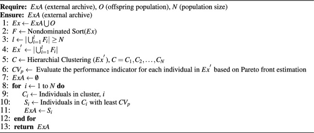
Update external archive
In each iteration of the evolutionary process, a critical fusion occurs where the archive population (ExA) and the offspring population (O) merge, resulting in a unified population denoted as Ex. This pivotal step lays the groundwork for the subsequent essential procedure: the non-dominated sorting of the Ex population. In Algorithm 4, the method for updating the external archive is described in detail. This systematic sorting process carefully organizes individuals into distinct non-dominated fronts, guided by their dominance relations. This systematic categorization effectively classifies individuals based on their performance and superiority over others. Like the truncation technique introduced in Ar-RGDEMO, individuals occupying the top l rank levels are specifically chosen to form a temporary population, identified as .
Following this initial selection, a refining process unfolds through hierarchical clustering applied to the temporary population . This clustering approach skillfully partitions individuals into N discrete clusters, thereby establishing subsets denoted as . Furthermore, an essential aspect of the process involves acquiring the performance metric, denoted as , for each individual within the temporary population . This metric is a critical measure of an individual’s effectiveness within the evolutionary framework. Subsequently, from each cluster , the individual demonstrating the most favorable performance metric, specifically the lowest value, is meticulously identified and preserved as a member of the external archive population. This meticulous selection process ensures that only the most promising and diverse individuals are included in the external archive, thus positioning them to play a pivotal role in guiding the evolutionary process toward optimal solutions.
Computational complexity analysis
The proposed Ar-RGDEMO algorithm comprises three critical components: (1) Radial-grid-based mutation, (2) Truncation procedure, and (3) External archive update. As previously outlined, the radial-grid-based mutation consists of three steps: constructing the radial grid, evaluating the performance indicator, and generating the perturbed vector. Constructing the radial grid has a computational complexity of O(MN), where M represents the number of objectives and N denotes the population size. The performance indicator evaluation requires ideal and nadir point estimations, each demanding O(MN) computations. An additional O(MN) calculation is necessary to assess the performance indicator. Generating the perturbed vector requires O(DN) calculations, where D is the number of decision variables.
Following the generation of trail vectors, DE one-to-one selection is performed. This process, which compares the quality of target vectors to their corresponding trail vectors, requires O(MN) computations and eliminates inferior solutions. For worst-case complexity analysis, we assume no solutions are eliminated during the DE one-to-one selection process. The nondominated sorting requires O(MNlogN/logM) computations in the truncation procedure. The ranking method based on shifted similarity distance involves computations for calculating shifted distances and O(NlogN) for ranking. Updating the external archive involves nondominated sorting, requiring O(MNlogN/logM) computations and clustering, which demands operations. Considering all these components, the overall worst-case computational complexity of Ar-RGDEMO is if ; otherwise, it is O(DN). This complexity arises from the most demanding operations in the algorithm, particularly those in the truncation procedure and external archive update.
Empirical studies
In this section, the experiments are structured into two distinct parts. The first part entails a comparative analysis, where Ar-RGDEMO is compared against state-of-the-art algorithms on benchmark problems. The primary aim is to illustrate and substantiate the efficacy of Ar-RGDEMO in attaining the desired levels of convergence and diversity. The second part of the experiments is dedicated to ablation studies to confirm the effectiveness of integrating an external archive.
Benchmark problems
In this study, we employ 30 test problems from widely used benchmark test suites, including ZDT (ZDT1-ZDT4, ZDT6)51, UF (UF1-UF10)52, IMOP (IMOP1-IMOP8)53, and MaF (MaF1-MaF7)54. These problems are utilized to evaluate the performance of the proposed Ar-RGDEMO approach against selected comparative algorithms. The number of decision variables employed varies across different problem sets. For ZDT1-ZDT3, the number of decision variables is set at 30, whereas for ZDT4 and ZDT6 problems, it is considered as 1051. As suggested in52, the number of decision variables for the entire UF test suite is set to 30. Regarding MaF1-MaF7 problems, the decision variable is , where M denotes the number of objectives. For MaF1-MaF6, K is set to 10, whereas for MaF7 problems, K is set to 2054. The 30 benchmark problems utilized in this paper exhibit various characteristics, including linearity, discontinuity, concavity, convexity, degeneracy, bias, mixed properties, non-separability, and multi-modality.
Quality metrics
To assess the performance of algorithms under comparison in this paper, we have employed two widely recognized performance metrics: modified inverted generational distance ()55 and hypervolume (HV)56. The metric evaluates the average modified distance from points within the Pareto front to their nearest solution within an approximation of the Pareto front. Mathematically, the metric is formulated as follows
| 8 |
where S denote the Pareto front approximated by the algorithms, represent the reference Pareto front, and denote the size of the reference Pareto front. The expression denotes the minimum of , signifying the adjusted distance from x to the nearest solution in S corresponding to point s. A low IGD+ value is commonly considered favorable, suggesting that the solution set closely approximates the Pareto front and exhibits substantial diversity55.
The Hypervolume (HV) metric quantifies the volume within the objective space, bounded by the obtained solution set and a predefined reference point. During the computation of HV, all reference points are standardized to 1.1 times the maximum value of each objective.
The hypervolume metric56 can be mathematically expressed as follows:
| 9 |
where represents the reference point, S denotes the approximated Pareto front, and signifies the Lebesgue measure. Further, higher HV values signify superior algorithmic performance.
Peer algorithms and parameter settings
In this study, to assess the efficacy of the proposed Ar-RGDEMO, we have chosen seven state-of-the-art algorithms as benchmarks. These include MOEAD-DE40, MOEAD-FRRMAB35, MOEAD-DYTS36, MOEAD-PaS41, RPEA57, SPEAR58, and MaOEA-IGD15. Among the selected algorithms, MOEAD-DE40 and MOEAD-PaS41 utilize a decomposition-based framework in conjunction with the DE operator to generate the offspring population. The algorithms MOEAD-FRRMAB35 and MOEAD-DYTS36 feature adaptive operator selection mechanisms, dynamically choosing from a range of DE operators to generate offspring. Finally, the RPEA57, SPEAR58, and MaOEA-IGD15 algorithms follow the MOEA framework. While RPEA and SPEAR utilize a reference point-based approach, MaOEA-IGD uses an indicator-based approach.
These algorithms were selected as comparison benchmarks for several compelling reasons. GA-based MOEAs (RPEA, SPEAR, and MaOEA-IGD) were chosen for their proven effectiveness and widespread adoption in solving MOPs. DE-based algorithms (MOEAD-FRRMAB and MOEAD-DYTS) enable performance analysis of the proposed algorithm using similar techniques. MOEAD-DE and MOEAD-PaS represent algorithms employing DE operators, allowing for a focused comparison with methods sharing similar evolutionary mechanisms but differing implementations. This diverse selection aims to comprehensively evaluate the proposed method against state-of-the-art techniques in multi-objective optimization. The proposed Ar-RGDEMO and the comparison algorithms were implemented utilizing PlatEMO59. The simulation experiments were conducted on a computer running a 64-bit operating system and powered by an 11th Gen Intel(R) Core(TM) i9-11900 processor.
To ensure a fair comparison, the parameters of the selected algorithms have been carefully calibrated to achieve optimal performance. In the case of MOEAD-DE, the neighborhood size is fixed at 20, with each offspring solution replacing two candidate solutions and a parent selection probability of 0.9. For the MOEAD-FRRMAB algorithm, the scaling factor is adjusted to 5, the decay factor to 1, and the sliding window size is determined as , with N representing the population size. In RPEA, the ratio of individuals utilized to generate reference points is also set to 0.4, with the parameter governing the difference between the reference point and the individuals set at 0.1. The remaining algorithms-SPEAR, MaOEA-IGD, MOEAD-PaS, and MOEAD-DYTS-are inherently parameter-free.
Evolutionary operator settings
The RPEA, SPEAR, and MaOEA-IGD algorithms employ the simulated binary crossover (SBX)60 and polynomial mutation47 to generate offspring populations. In contrast, the MOEAD-DE, MOEAD-FRRMAB, MOEAD-DYTS, and MOEAD-PaS algorithms utilize the DE operator42 with the polynomial mutation to create offspring populations. Table 2 outlines the parameter configurations for the evolutionary operators utilized within the chosen algorithms.
Table 2.
Parameters of evolutionary operators adopted in the algorithms. (crossover index); (crossover probability); CR (crossover rate); F (scaling factor); (mutation index); (mutation probability).
| Algorithm | CR | F | ||||
|---|---|---|---|---|---|---|
| RPEA, SPEAR, & MaOEA-IGD | 20 | 1 | - | - | 20 | 1/n |
| MOEAD-DE, MOEAD-FRRMAB, MOEAD-DYTS, & MOEAD-PaS | - | - | 0.3 | 0.5 | 20 | 1/n |
| Ar-RGDEMO | - | - | 0.3 | 0.5 | 20 | 1/n |
Experimental settings
Number of objectives
The chosen test suites encompass various problems, including the ZDT test suite, UF1-UF7, and IMOP1-IMOP3, each featuring two objectives. Conversely, UF8-UF10 and IMOP4-IMOP8 problems are characterized by three objectives. Additionally, within the MaF problem suites, test instances with 3, 5, 8, and 10 objectives were integrated.
Population size
The population sizes for problems with 2, 3, 5, 8, and 10 objectives are correspondingly established as 100, 105, 126, 156, and 275. These sizes adhere to recommendations provided in prior studies such as15,57,58.
Function evaluations and simulation runs
The chosen algorithms undergo independent simulation across 30 runs. The function evaluations for each test instance are displayed in Table 3.
Table 3.
Function evaluations for benchmark problems.
| Problem | |||||
|---|---|---|---|---|---|
| ZDT1-ZDT3 & ZDT6 | 50,000 | - | - | - | - |
| ZDT4 & UF1-UF7 | 100,000 | - | - | - | - |
| UF8-UF10 | - | 100,000 | - | - | - |
| IMOP1-IMOP2 | 200,000 | - | - | - | - |
| IMOP3 | 250,000 | - | - | - | - |
| IMOP4-5 & IMOP8 | - | 200,000 | - | - | - |
| IMOP6-7 | - | 250,000 | - | - | - |
| MaF1 & MaF4-MaF6 | - | 105,000 | 126,000 | 156000 | 275,000 |
| MaF2 & MaF3 & MaF7 | - | 126,000 | 160,650 | 195,000 | 385,000 |
Significance test
The chosen algorithms undergo independent simulation across 30 runs. Table 3 displays the function evaluations for each test instance.
Experimental results
This section offers a comprehensive presentation and analysis of the results of various competing algorithms across test problems characterized by specific objectives. These results are obtained with selected quality metrics presented in Tables 4, 5, 6 and 7 to highlight the distinctive performance of the proposed algorithm in addressing MOPs and MaOPs compared to the algorithms chosen for evaluation. The null hypothesis is rejected in the Wilcoxon rank-sum test, conducted at a significance level 0.05. Within the tables, symbols such as , −, and convey the relative performance of the compared state-of-the-art algorithms concerning the proposed Ar-RGDEMO. Specifically, indicates significantly better performance, − denotes substantially worse performance, and signifies statistical similarity in performance.
Table 4.
Mean and standard deviation values of metric for Ar-RGDEMO and state-of-art algorithms on ZDT, UF and IMOP benchmark problems.
| Problem | M | MOEAD-DE | MOEAD-FRRMAB | MOEAD-DYTS | MOEAD-PaS | RPEA | SPEAR | MaOEA-IGD | Ar-RGDEMO |
|---|---|---|---|---|---|---|---|---|---|
| ZDT1 | 2 | 4.70e-3 (9.07e-4)− | 3.32e-3 (5.12e-4)− | 3.39e-3 (4.36e-4)− | 8.83e-3 (2.72e-3)− | 7.69e-3 (5.40e-4)− | 3.27e-3 (2.82e-4)− | 2.75e-1 (4.32e-2)− | 2.94e-3 (7.70e-5) |
| ZDT2 | 2 | 3.46e-3 (4.77e-4)− | 2.80e-3 (2.58e-4)− | 2.68e-3 (1.66e-4) | 1.71e+0 (1.57e+0)− | 8.97e-3 (1.23e-3)− | 3.17e-3 (2.72e-4)− | 3.83e-1 (6.66e-2)− | 2.64e-3 (8.33e-5) |
| ZDT3 | 2 | 4.16e-3 (2.96e-4)− | 4.67e-3 (1.26e-3)− | 3.93e-3 (3.04e-4)− | 6.25e-3 (2.05e-3)− | 7.22e-3 (6.34e-3)− | 2.63e-3 (5.31e-4)− | 2.23e-1 (2.45e-2)− | 1.98e-3 (1.85e-4) |
| ZDT4 | 2 | 3.00e-3 (3.52e-4)− | 2.74e-3 (2.34e-4) | 2.56e-3 (5.46e-5) | 2.74e+1 (2.13e+1)− | 8.53e-3 (9.19e-4)− | 3.66e-3 (3.01e-3)− | 3.64e-1 (8.97e-2)− | 2.76e-3 (5.23e-5) |
| ZDT6 | 2 | 2.08e-3 (9.96e-6) | 2.09e-3 (1.32e-5) | 2.08e-3 (9.32e-6) | 2.26e-3 (5.60e-4) | 7.23e-3 (2.01e-3)− | 2.89e-3 (5.46e-4)− | 2.77e-1 (8.91e-2)− | 2.33e-3 (5.97e-5) |
| UF1 | 2 | 1.93e-2 (1.96e-2) | 1.61e-2 (4.94e-3) | 9.64e-3 (8.68e-4) | 1.93e-2 (2.56e-2) | 7.53e-2 (2.14e-2)− | 6.95e-2 (1.40e-2)− | 3.49e-1 (1.12e-1)− | 3.63e-2 (8.71e-3) |
| UF2 | 2 | 2.55e-2 (1.81e-2)− | 1.63e-2 (2.02e-3)− | 1.49e-2 (2.20e-3) | 1.92e-2 (9.95e-3)− | 4.46e-2 (1.18e-2)− | 2.62e-2 (6.39e-3)− | 2.31e-1 (1.43e-2)− | 1.46e-2 (1.48e-3) |
| UF3 | 2 | 1.04e-1 (5.98e-2) | 2.90e-2 (1.77e-2) | 2.74e-2 (1.45e-2) | 1.07e-1 (2.04e-1) | 2.10e-1 (1.27e-2)− | 1.42e-1 (2.48e-2)− | 1.12e+0 (3.34e-1)− | 1.14e-1 (1.30e-2) |
| UF4 | 2 | 8.01e-2 (6.57e-3)− | 6.60e-2 (6.69e-3)− | 5.31e-2 (3.41e-3)− | 7.57e-2 (7.91e-3)− | 6.18e-2 (6.06e-3)− | 4.65e-2 (1.48e-3)− | 3.68e-1 (1.77e-1)− | 4.33e-2 (2.34e-3) |
| UF5 | 2 | 4.80e-1 (9.03e-2)− | 5.02e-1 (1.09e-1)− | 4.77e-1 (6.57e-2)− | 5.58e-1 (1.02e-1)− | 3.01e-1 (1.14e-1) | 2.81e-1 (7.88e-2) | 3.31e+0 (1.29e+0)− | 2.51e-1 (7.85e-2) |
| UF6 | 2 | 2.58e-1 (1.24e-1)− | 2.59e-1 (1.91e-1)− | 3.58e-1 (6.62e-2)− | 1.88e-1 (1.47e-1)− | 1.83e-1 (8.68e-2)− | 1.33e-1 (7.56e-2) | 2.78e+0 (1.73e+0)− | 1.16e-1 (4.73e-2) |
| UF7 | 2 | 4.90e-2 (1.10e-1)− | 2.89e-2 (8.40e-2) | 2.52e-1 (2.29e-1) | 1.43e-2 (4.42e-3) | 1.84e-1 (1.11e-1)− | 1.32e-1 (1.09e-1)− | 4.41e-1 (1.53e-1)− | 2.91e-2 (4.68e-2) |
| UF8 | 3 | 1.51e-1 (5.74e-2) | 1.56e-1 (6.99e-2) | 2.08e-1 (1.67e-1) = | 1.52e-1 (8.11e-2)− | 2.29e-1 (9.95e-4)− | 1.62e-1 (7.25e-2)− | 5.24e-1 (6.11e-3)− | 1.51e-1 (8.31e-2) |
| UF9 | 3 | 2.20e-1 (4.56e-2)− | 2.27e-1 (8.52e-3)− | 2.16e-1 (5.16e-2)− | 2.17e-1 (4.09e-2)− | 3.87e-1 (6.60e-2)− | 2.17e-1 (1.09e-1)− | 5.616e-1 (9.11e-2)− | 1.14e-1 (5.64e-2) |
| UF10 | 3 | 6.72e-1 (1.07e-1) | 1.02e+0 (2.03e-1)− | 6.98e-1 (8.84e-2) | 5.95e-1 (8.39e-2) | 3.90e-1 (1.20e-1) | 3.39e-1 (6.86e-2) | 1.68e+0 (1.24e+0)− | 6.78e-1 (1.13e-1) |
| IMOP1 | 2 | 2.07e-3 (2.80e-5)− | 2.04e-3 (3.65e-5)− | 2.05e-3 (1.32e-5)− | 7.12e-1 (1.04e-2)− | 2.96e-3 (7.42e-4)− | 1.85e-3 (1.84e-4)− | 2.10e-2 (1.58e-4)− | 3.93e-4 (2.00e-5) |
| IMOP2 | 2 | 1.78e-3 (8.95e-5)− | 1.76e-3 (8.92e-5)− | 1.77e-3 (1.06e-4)− | 2.33e-1 (1.41e-1)− | 5.14e-3 (1.00e-3)− | 1.37e-3 (8.48e-5)− | 3.11e-1 (8.44e-2)− | 1.19e-3 (8.10e-5) |
| IMOP3 | 2 | 3.16e-3 (4.98e-4) | 3.71e-3 (4.09e-4) | 3.74e-3 (4.05e-4) | 4.65e-1 (1.57e-1)− | 1.52e-2 (8.09e-3) | 2.16e-3 (1.75e-4) | 4.70e-1 (6.31e-2)− | 1.98e-2 (7.00e-3) |
| IMOP4 | 3 | 8.93e-3 (1.45e-5)− | 8.92e-3 (2.52e-5)− | 8.93e-3 (4.19e-5)− | 1.34e-2 (1.00e-3)− | 7.84e-3 (5.19e-4)− | 2.11e-2 (1.28e-3)− | 5.38e-1 (8.56e-2)− | 5.54e-3 (4.24e-4) |
| IMOP5 | 3 | 4.03e-2 (5.65e-3) | 4.01e-2 (5.39e-3) | 4.01e-2 (5.52e-3) | 3.18e-1 (2.09e-1)− | 3.98e-2 (3.63e-3) | 3.53e-2 (6.44e-4) | 4.04e-1 (2.82e-4)− | 5.02e-2 (1.58e-2) |
| IMOP6 | 3 | 3.24e-2 (3.12e-4) | 3.30e-2 (5.70e-4) | 3.28e-2 (4.48e-4) | 3.49e-2 (8.83e-4) | 1.33e-1 (8.98e-2)− | 2.87e-2 (5.69e-4) | 8.98e-2 (4.67e-2)− | 4.30e-2 (6.81e-2) |
| IMOP7 | 3 | 2.60e-2 (7.41e-4) | 2.84e-2 (9.06e-4) | 2.83e-2 (8.09e-4) | 8.84e-2 (1.21e-1) | 4.98e-1 (8.96e-2) | 2.10e-2 (1.70e-4) | 5.14e-1 (1.33e-5) | 3.42e-1 (2.35e-1) |
| IMOP8 | 3 | 1.48e-1 (6.07e-3)− | 1.46e-1 (4.87e-3)− | 1.43e-1 (3.21e-3)− | 4.43e-2 (2.84e-3)− | 2.32e-1 (1.56e-1)− | 6.31e-2 (2.58e-3)− | 4.14e-1 (2.08e-1)− | 2.49e-2 (1.86e-3) |
| 5/14/4 | 8/13/2 | 7/10/6 | 7/16/0 | 3/18/2 | 5/16/2 | 0/22/1 | |||
Significant values are in bold.
Table 5.
Mean and standard deviation values of metric for Ar-RGDEMO and state-of-art algorithms on MaF benchmark problems.
| Problem | M | MOEAD-DE | MOEAD-FRRMAB | MOEAD-DYTS | MOEAD-PaS | RPEA | SPEAR | MaOEA-IGD | Ar-RGDEMO |
|---|---|---|---|---|---|---|---|---|---|
| MaF1 | 3 | 4.64e-2 (9.47e-3)− | 4.45e-2 (2.50e-4)− | 4.42e-2 (1.98e-4)− | 6.53e-2 (1.15e-3)− | 6.95e-2 (1.89e-2)− | 4.41e-2 (1.18e-3)− | 1.29e-1 (4.19e-4)− | 2.99e-2 (3.64e-4) |
| 5 | 1.35e-1 (1.70e-3)− | 1.36e-1 (2.02e-3)− | 1.32e-1 (2.02e-3)− | 1.39e-1 (7.98e-4)− | 1.45e-1 (1.04e-2)− | 1.54e-1 (2.57e-3)− | 2.38e-1 (2.05e-3)− | 8.89e-2 (9.82e-4) | |
| 8 | 2.21e-1 (4.67e-3)− | 2.18e-1 (4.28e-3)− | 2.02e-1 (6.29e-3)− | 1.98e-1 (5.92e-3)− | 2.07e-1 (5.73e-3)− | 2.93e-1 (3.39e-2)− | 3.05e-1 (4.94e-3)− | 1.60e-1 (1.97e-3) | |
| 10 | 2.29e-1 (4.60e-3)− | 2.42e-1 (4.89e-3)− | 2.30e-1 (4.66e-3)− | 2.01e-1 (4.42e-3)− | 2.11e-1 (4.21e-3)− | 3.33e-1 (2.00e-2)− | 2.94e-1 (2.84e-3)− | 1.65e-1 (1.23e-3) | |
| MaF2 | 3 | 2.86e-2 (1.05e-3)− | 2.78e-2 (7.76e-4)− | 2.75e-2 (1.08e-3)− | 2.89e-2 (8.02e-4)− | 3.43e-2 (2.35e-3)− | 2.40e-2 (7.25e-4)− | 1.50e-1 (1.02e-1)− | 1.91e-2 (3.52e-4) |
| 5 | 1.10e-1 (3.23e-3)− | 1.12e-1 (3.43e-3)− | 1.12e-1 (3.70e-3)− | 1.31e-1 (4.87e-3)− | 7.33e-2 (2.23e-3)− | 9.39e-2 (1.68e-3)− | 9.32e-2 (5.09e-2)− | 5.99e-2 (2.02e-3) | |
| 8 | 1.84e-1 (5.53e-3)− | 1.84e-1 (5.81e-3)− | 1.82e-1 (6.28e-3)− | 4.14e-1 (3.52e-2)− | 1.07e-1 (3.57e-3) | 1.37e-1 (4.13e-4)− | 1.91e-1 (1.03e-2− | 1.19e-1 (5.97e-3) | |
| 10 | 1.77e-1 (5.74e-3)− | 1.74e-1 (4.86e-3)− | 1.72e-1 (4.94e-3− | 4.75e-1 (1.17e-2)− | 1.07e-1 (3.74e-3) | 1.39e-1 (5.44e-3− | 2.01e-1 (7.79e-3)− | 1.16e-1 (3.97e-3) | |
| MaF3 | 3 | 4.59e-2 (3.43e-3)− | 5.23e-2 (5.22e-2)− | 1.20e-1 (3.94e-1)− | 2.30e+0 (8.53e+0)− | 1.06e-1 (2.87e-2)− | 1.56e-1 (1.57e-1)− | 1.40e+3 (6.24e+3)− | 1.65e-2 (6.20e-4) |
| 5 | 2.17e-1 (5.75e-1)− | 1.87e+0 (7.47e+0)− | 6.90e-1 (1.79e+0)− | 1.17e+3 (3.89e+3)− | 2.99e-1 (9.20e-2)− | 7.24e-1 (1.81e+0)− | 3.34e+1 (4.77e+1)− | 4.98e-2 (5.73e-2) | |
| 8 | 4.63e-2 (8.77e-3) | 5.82e-2 (8.12e-2) + | 4.49e-2 (1.25e-2) | 6.78e+3 (1.53e+4)− | 3.61e-1 (1.14e-1) | 9.18e+3 (1.59e+4)− | 8.17e+0 (1.11e+1)− | 1.69e+0 (7.42e+0) | |
| 10 | 3.03e-2 (3.33e-3) | 2.86e-2 (1.87e-3) | 2.93e-2 (2.27e-3) | 6.64e+4 (3.19e+5)− | 2.81e-1 (1.26e-1)− | 8.85e+4 (1.21e+5)− | 1.45e+0 (2.78e+0)− | 3.55e-2 (1.25e-2) | |
| MaF4 | 3 | 4.06e-1 (1.06e+0)− | 2.09e-1 (2.10e-2)− | 2.01e-1 (2.49e-2)− | 2.28e-1 (4.45e-1)− | 1.67e-1 (2.68e-2)− | 7.81e-1 (5.34e-1)− | 4.38e+0 (6.18e+0)− | 1.04e-1 (5.53e-3) |
| 5 | 1.71e+0 (7.07e-2)− | 7.59e+0 (1.85e+1)− | 2.14e+0 (2.77e+0)− | 3.19e+0 (7.20e+0)− | 7.93e-1 (7.96e-2)− | 4.16e+0 (1.10e+0)− | 1.38e+1 (1.90e+1)− | 6.52e-1 (2.05e-2) | |
| 8 | 9.11e+0 (9.79e+0)− | 7.51e+1 (1.17e+2)− | 7.67e+0 (1.96e+0)− | 1.92e+1 (1.13e+0)− | 6.58e+0 (5.60e+0)− | 3.51e+1 (3.00e+1)− | 7.24e+1 (6.58e+1)− | 2.88e+0 (7.46e-2) | |
| 10 | 2.28e+1 (1.21e+0)− | 1.37e+2 (3.16e+2)− | 2.26e+1 (1.25e+0)− | 6.81e+1 (3.77e+0)− | 1.50e+1 (4.06e+0)− | 1.15e+2 (1.12e+2)− | 1.02e+2 (1.97e+2)− | 6.71e+0 (1.69e-1) | |
| MaF5 | 3 | 1.84e-1 (2.30e-2)− | 1.73e-1 (6.06e-3)− | 1.76e-1 (1.14e-2)− | 7.94e-1 (1.21e+0)− | 1.20e+0 (1.56e+0)− | 8.07e-2 (2.41e-3) + | 3.42e-1 (2.19e-1)− | 1.44e-1 (1.98e-1) |
| 5 | 8.87e-1 (1.25e-2)− | 8.91e-1 (1.32e-2)− | 8.88e-1 (1.34e-2)− | 5.37e-1 (3.25e-2) + | 2.19e+0 (3.92e+0)− | 4.19e-1 (8.67e-3) + | 6.995e-1 (1.45e-1)− | 5.44e-1 (1.37e-2) | |
| 8 | 1.33e+0 (2.60e-2) | 1.32e+0 (1.97e-2) | 1.32e+0 (2.14e-2) | 9.93e-1 (4.90e-2) | 1.26e+0 (4.14e-1) | 9.60e-1 (1.29e-2) | 1.13e+0 (1.09e-1) | 8.48e+0 (1.27e+0) | |
| 10 | 1.47e+0 (2.80e-2) | 1.43e+0 (2.81e-2) | 1.44e+0 (2.63e-2) | 1.12e+0 (3.46e-2) | 1.24e+0 (2.62e-2) | 1.11e+0 (1.39e-2) | 1.14e+0 (4.27e-2) | 2.20e+1 (4.31e+0) | |
| MaF6 | 3 | 4.69e-3 (3.23e-5)− | 4.67e-3 (3.32e-5)− | 4.64e-3 (1.63e-5)− | 8.69e-3 (9.75e-4)− | 1.04e-2 (1.70e-3)− | 1.39e-2 (7.55e-4)− | 3.56e-1 (7.42e-2)− | 1.84e-3 (4.93e-5) |
| 5 | 1.23e-2 (4.27e-5)− | 1.22e-2 (1.41e-5)− | 1.22e-2 (1.24e-5)− | 5.74e-2 (8.80e-3)− | 8.41e-3 (1.58e-3)− | 4.12e-2 (6.36e-3)− | 3.45e-1 (7.30e-2)− | 1.55e-3 (3.56e-5) | |
| 8 | 8.92e-3 (4.85e-5) | 8.85e-3 (2.58e-5) | 8.83e-3 (1.18e-5) | 4.06e-1 (5.11e-2) | 7.94e-3 (1.84e-3) | 6.46e-2 (6.45e-2) | 3.47e-1 (8.93e-2) | 2.69e+0 (1.56e+0) | |
| 10 | 9.87e-3 (3.79e-5) | 9.81e-3 (2.93e-5) | 9.79e-3 (2.63e-5) | 3.92e-1 (4.19e-2) | 6.98e-3 (2.39e-3) | 7.30e-2 (2.61e-2) | 3.39e-1 (9.72e-2) | 2.91e+0 (1.60e+0) | |
| MaF7 | 3 | 1.50e-1 (1.49e-1)− | 9.01e-2 (1.48e-3)− | 9.06e-2 (1.23e-3)− | 1.56e+0 (2.31e+0)− | 3.43e-1 (2.73e-1)− | 4.00e-2 (1.47e-3)− | 6.37e-1 (4.52e-1)− | 2.96e-2 (8.61e-4) |
| 5 | 3.70e-1 (7.50e-2)− | 3.07e-1 (5.94e-2)− | 3.68e-1 (7.43e-2)− | 5.87e-1 (1.28e+0)− | 8.37e-1 (3.13e-1)− | 2.10e-1 (7.32e-3) | 1.22e+0 (1.22e+0)− | 2.23e-1 (1.62e-1) | |
| 8 | 8.12e-1 (5.56e-2)− | 8.16e-1 (5.81e-2)− | 8.34e-1 (6.55e-2)− | 2.35e+0 (8.44e-1)− | 1.75e+0 (3.67e-1)− | 7.67e-1 (2.34e-2)− | 9.24e-1 (1.14e+0)− | 4.76e-1 (1.50e-1) | |
| 10 | 1.06e+0 (4.08e-2)− | 1.14e+0 (5.15e-2)− | 1.14e+0 (3.89e-2)− | 3.10e+0 (6.44e-1)− | 1.49e+0 (2.31e-1)− | 1.78e+0 (9.30e-2)− | 8.87e-1 (4.85e-2)− | 7.49e-1 (3.13e-2) | |
| 4/22/2 | 6/22/0 | 6/22/0 | 5/23/0 | 7/21/0 | 7/21/0 | 4/24/0 | |||
Significant values are in bold.
Table 6.
Mean and standard deviation values of HV metric for Ar-RGDEMO and state-of-art algorithms on ZDT, UF and IMOP benchmark problems.
| Problem | M | MOEAD-DE | MOEAD-FRRMAB | MOEAD-DYTS | MOEAD-PaS | RPEA | SPEAR | MaOEA-IGD | Ar-RGDEMO |
|---|---|---|---|---|---|---|---|---|---|
| ZDT1 | 2 | 7.17e-1 (1.35e-3)− | 7.19e-1 (7.88e-4)− | 7.19e-1 (6.63e-4)− | 7.11e-1 (3.85e-3)− | 7.11e-1 (1.14e-3)− | 7.19e-1 (7.19e-4)− | 3.04e-1 (6.26e-2)− | 7.20e-1 (1.04e-4) |
| ZDT2 | 2 | 4.42e-1 (1.11e-3)− | 4.44e-1 (4.30e-4) | 4.44e-1 (3.31e-4) | 1.88e-1 (2.19e-1)− | 4.35e-1 (1.54e-3)− | 4.43e-1 (7.65e-4)− | 1.02e-1 (2.72e-2)− | 4.44e-1 (2.22e-4) |
| ZDT3 | 2 | 5.98e-1 (6.01e-4)− | 5.96e-1 (1.74e-3)− | 5.97e-1 (5.09e-4)− | 5.99e-1 (1.73e-3) | 6.06e-1 (2.82e-2) | 5.98e-1 (1.49e-3)− | 4.68e-1 (9.37e-2)− | 6.00e-1 (1.49e-3) |
| ZDT4 | 2 | 7.19e-1 (5.61e-4)− | 7.20e-1 (3.55e-4)− | 7.20e-1 (9.08e-5)− | 1.19e-1 (2.71e-1)− | 7.11e-1 (1.25e-3)− | 7.18e-1 (3.87e-3)− | 1.85e-1 (9.74e-2)− | 7.20e-1 (6.88e-5) |
| ZDT6 | 2 | 3.89e-1 (1.53e-4) | 3.89e-1 (2.62e-4) | 3.89e-1 (1.34e-4) | 3.89e-1 (8.77e-4) | 3.81e-1 (2.81e-3)− | 3.87e-1 (1.21e-3) | 1.21e-1 (5.40e-2)− | 3.88e-1 (3.84e-4) |
| UF1 | 2 | 6.93e-1 (2.65e-2) | 6.99e-1 (7.07e-3) | 7.09e-1 (1.16e-3) | 6.96e-1 (2.67e-2) | 5.88e-1 (3.28e-2)− | 6.03e-1 (2.31e-2)− | 2.42e-1 (1.03e-1)− | 6.62e-1 (1.77e-2) |
| UF2 | 2 | 6.90e-1 (2.00e-2)− | 7.01e-1 (2.32e-3)− | 7.02e-1 (2.85e-3) | 6.97e-1 (1.11e-2)− | 6.61e-1 (1.18e-2)− | 6.87e-1 (7.75e-3)− | 3.8558e-1 (2.41e-2)− | 7.03e-1 (2.90e-3) |
| UF3 | 2 | 5.57e-1 (1.02e-1) | 6.78e-1 (2.61e-2) | 6.80e-1 (2.15e-2) | 5.95e-1 (1.93e-1) | 3.91e-1 (2.05e-2)− | 4.90e-1 (3.70e-2)− | 1.24e-3 (6.79e-3)− | 5.64e-1 (1.36e-2) |
| UF4 | 2 | 3.33e-1 (8.29e-3)− | 3.53e-1 (9.01e-3)− | 3.67e-1 (5.24e-3)− | 3.39e-1 (1.06e-2)− | 3.45e-1 (1.12e-2)− | 3.78e-1 (2.49e-3)− | 1.20e-1 (1.02e-1)− | 3.84e-1 (3.56e-3) |
| UF5 | 2 | 9.98e-2 (6.60e-2)− | 6.22e-2 (7.12e-2)− | 8.69e-2 (1.28e-2)− | 3.52e-2 (3.50e-2)− | 2.23e-1 (8.19e-2) | 2.21e-1 (6.98e-2) | 0.00e+0 (0.00e+0)− | 2.35e-1 (7.88e-2) |
| UF6 | 2 | 2.60e-1 (8.64e-2)− | 2.52e-1 (1.05e-1)− | 1.06e-1 (6.08e-2)− | 3.11e-1 (8.04e-2) | 2.79e-1 (7.20e-2)− | 3.36e-1 (6.95e-2) | 2.80e-4 (1.54e-3)− | 3.49e-1 (3.70e-2) |
| UF7 | 2 | 5.26e-1 (1.09e-1)− | 5.49e-1 (8.20e-2) | 3.32e-1 (2.25e-1) | 5.62e-1 (7.98e-3) | 3.72e-1 (1.04e-1)− | 4.32e-1 (1.12e-1)− | 1.43e-1 (9.94e-2)− | 5.42e-1 (4.78e-2) |
| UF8 | 3 | 3.49e-1 (3.88e-2)− | 3.50e-1 (4.60e-2)− | 3.08e-1 (1.14e-1)− | 3.81e-1 (5.70e-2)− | 3.37e-1 (2.33e-3)− | 3.64e-1 (5.38e-2)− | 8.51e-2 (7.64e-3)− | 4.01e-1 (6.41e-2) |
| UF9 | 3 | 5.73e-1 (4.26e-2)− | 5.61e-1 (1.56e-2)− | 5.61e-1 (3.99e-2)− | 5.81e-1 (4.89e-2)− | 3.49e-1 (6.46e-2)− | 5.41e-1 (1.16e-1)− | 1.65e-1 (7.52e-2)− | 6.78e-1 (4.47e-2) |
| UF10 | 3 | 3.90e-2 (3.05e-2) | 8.30e-4 (3.12e-3)− | 6.97e-3 (1.24e-2) | 5.76e-2 (3.22e-2) | 1.73e-1 (9.50e-2) | 1.67e-1 (4.05e-2) | 5.71e-3 (1.66e-2) | 5.43e-3 (1.13e-2) |
| IMOP1 | 2 | 9.85e-1 (4.34e-5)− | 9.85e-1 (5.65e-5)− | 9.85e-1 (2.04e-5)− | 1.09e-1 (9.62e-3)− | 9.83e-1 (1.17e-3)− | 9.85e-1 (3.06e-4)− | 9.49e-1 (2.16e-4)− | 9.87e-1 (4.31e-5) |
| IMOP2 | 2 | 2.31e-1 (1.35e-4)− | 2.31e-1 (1.35e-4)− | 2.31e-1 (1.60e-4)− | 1.15e-1 (6.93e-2)− | 2.25e-1 (1.78e-3)− | 2.31e-1 (3.91e-4)− | 8.57e-2 (2.67e-2)− | 2.32e-1 (1.22e-4) |
| IMOP3 | 2 | 6.57e-1 (5.80e-4) | 6.56e-1 (4.85e-4) | 6.56e-1 (4.96e-4) | 1.43e-1 (1.75e-1)− | 6.40e-1 (1.22e-2) | 6.58e-1 (5.10e-4) | 1.42e-1 (6.39e-2)− | 6.31e-1 (1.01e-2) |
| IMOP4 | 3 | 4.30e-1 (2.29e-5)− | 4.30e-1 (4.72e-5)− | 4.30e-1 (3.49e-5)− | 4.23e-1 (2.22e-3)− | 4.30e-1 (6.73e-4)− | 4.14e-1 (3.90e-3)− | 4.99e-2 (4.23e-2)− | 4.32e-1 (6.37e-4) |
| IMOP5 | 3 | 5.16e-1 (1.53e-2)− | 5.14e-1 (1.54e-2)− | 5.15e-1 (1.53e-2)− | 3.48e-1 (1.29e-1)− | 4.82e-1 (4.97e-3)− | 4.94e-1 (4.76e-3)− | 4.33e-1 (8.03e-4)− | 5.26e-1 (1.10e-2) |
| IMOP6 | 3 | 5.12e-1 (4.87e-4) | 5.11e-1 (7.91e-4) | 5.11e-1 (5.63e-4) | 5.10e-1 (8.96e-4) | 4.16e-1 (7.87e-2)− | 5.16e-1 (1.06e-3) | 4.60e-1 (4.29e-2)− | 5.00e-1 (6.87e-2) |
| IMOP7 | 3 | 4.99e-1 (1.72e-3) | 4.94e-1 (2.18e-3) | 4.94e-1 (1.95e-3) | 4.48e-1 (1.19e-1) | 1.09e-1 (7.42e-2) | 5.20e-1 (1.57e-4) | 9.52e-2 (1.62e-5) | 2.36e-1 (1.98e-1) |
| IMOP8 | 3 | 4.10e-1 (5.18e-3)− | 4.12e-1 (3.89e-3)− | 4.15e-1 (2.79e-3)− | 5.09e-1 (5.01e-3)− | 4.41e-1 (6.50e-2)− | 5.22e-1 (2.64e-3)− | 3.18e-1 (1.77e-1)− | 5.35e-1 (3.79e-3) |
| 6/16/1 | 7/15/1 | 6/13/4 | 7/14/2 | 3/18/2 | 4/16/3 | 1/21/1 | |||
Significant values are in bold.
Table 7.
Mean and standard deviation values of HV metric for Ar-RGDEMO and state-of-art algorithms on MaF benchmark problems.
| Problem | M | MOEAD-DE | MOEAD-FRRMAB | MOEAD-DYTS | MOEAD-PaS | RPEA | SPEAR | MaOEA-IGD | Ar-RGDEMO |
|---|---|---|---|---|---|---|---|---|---|
| MaF1 | 3 | 2.06e-1 (1.06e-2)− | 2.08e-1 (2.48e-4)− | 2.08e-1 (2.06e-4)− | 1.83e-1 (1.28e-3)− | 1.80e-1 (1.73e-2)− | 2.01e-1 (1.34e-3)− | 1.44e-1 (3.05e-4)− | 2.20e-1 (4.33e-4) |
| 5 | 6.00e-3 (1.74e-4)− | 5.89e-3 (1.75e-4)− | 6.26e-3 (1.69e-4)− | 5.57e-3 (7.33e-5)− | 5.29e-3 (6.62e-4)− | 5.17e-3 (1.64e-4)− | 3.73e-3 (9.31e-5)− | 1.05e-2 (1.54e-4) | |
| 8 | 2.27e-6 (1.49e-6)− | 2.68e-6 (1.98e-6)− | 3.89e-6 (2.08e-6)− | 2.74e-5 (1.50e-6) | 7.07e-6 (2.90e-6)− | 8.88e-6 (6.36e-6)− | 9.62e-6 (7.95e-7)− | 2.85e-5 (3.34e-6) | |
| 10 | 0.00e+0 (0.00e+0)− | 6.67e-8 (2.54e-7)− | 3.33e-8 (1.83e-7)− | 5.27e-7 (2.77e-8) | 1.67e-7 (3.79e-7)− | 3.42e-8 (1.50e-8)− | 1.32e-7 (1.25e-8)− | 5.58e-7 (2.66e-7) | |
| MaF2 | 3 | 2.30e-1 (2.59e-3)− | 2.29e-1 (2.13e-3)− | 2.30e-1 (2.64e-3)− | 2.36e-1 (8.07e-4)− | 2.30e-1 (1.73e-3)− | 2.38e-1 (1.23e-3)− | 1.28e-1 (7.10e-2)− | 2.39e-1 (1.82e-3) |
| 5 | 1.22e-1 (4.08e-3)− | 1.20e-1 (3.94e-3)− | 1.21e-1 (4.65e-3)− | 9.91e-2 (5.38e-3)− | 1.75e-1 (1.87e-3) | 1.53e-1 (2.43e-3)− | 1.48e-1 (2.83e-2)− | 1.62e-1 (4.48e-3) | |
| 8 | 1.73e-1 (2.45e-3) | 1.75e-1 (2.61e-3) | 1.75e-1 (3.03e-3) | 8.10e-2 (2.03e-2)− | 2.16e-1 (3.14e-3) | 1.79e-1 (2.13e-3) | 1.81e-1 (6.82e-3) | 1.66e-1 (7.55e-3) | |
| 10 | 1.82e-1 (2.05e-3) | 1.82e-1 (2.43e-3) | 1.82e-1 (1.91e-3) | 5.08e-2 (5.77e-3)− | 2.22e-1 (2.17e-3) | 1.82e-1 (1.65e-3) | 1.81e-1 (6.36e-3) | 1.58e-1 (9.36e-3) | |
| MaF3 | 3 | 9.27e-1 (8.57e-3)− | 9.20e-1 (8.22e-2)− | 8.96e-1 (1.70e-1)− | 8.60e-1 (2.52e-1)− | 8.46e-1 (2.56e-2)− | 7.72e-1 (2.13e-1)− | 0.00e+0 (0.00e+0)− | 9.62e-1 (6.10e-4) |
| 5 | 9.33e-1 (2.00e-1)− | 7.61e-1 (3.86e-1)− | 8.38e-1 (3.43e-1)− | 4.27e-1 (4.69e-1)− | 8.07e-1 (7.41e-2) − | 6.65e-1 (2.45e-1)− | 3.94e-2 (1.39e-1)− | 9.81e-1 (7.78e-2) | |
| 8 | 9.99e-1 (6.19e-4) | 9.88e-1 (6.33e-2) | 9.99e-1 (2.48e-3) | 7.71e-2 (2.07e-1)− | 8.14e-1 (9.79e-2) | 0.00e+0 (0.00e+0)− | 3.15e-2 (1.04e-1)− | 8.17e-1 (2.34e-1) | |
| 10 | 9.99e-1 (6.31e-5) | 9.99e-1 (1.43e-5) | 9.99e-1 (3.15e-5) | 3.94e-2 (1.45e-1)− | 8.92e-1 (9.23e-2) | 0.00e+0 (0.00e+0)− | 5.36e-1 (3.64e-1)− | 9.23e-1 (3.76e-2) | |
| MaF4 | 3 | 4.65e-1 (8.83e-2)− | 4.82e-1 (1.36e-2)− | 4.88e-1 (1.43e-2)− | 4.99e-1 (9.46e-2)− | 5.06e-1 (7.23e-3)− | 2.96e-1 (1.28e-1)− | 6.68e-2 (7.78e-2)− | 5.36e-1 (1.45e-3) |
| 5 | 1.56e-2 (3.35e-3)− | 1.53e-2 (7.74e-3)− | 1.82e-2 (4.84e-3)− | 4.34e-2 (8.52e-3)− | 9.74e-2 (5.99e-3)− | 1.76e-2 (1.37e-2)− | 1.38e-3 (2.54e-3)− | 1.13e-1 (1.59e-3) | |
| 8 | 2.70e-5 (1.42e-5)− | 1.57e-5 (1.85e-5)− | 2.96e-5 (1.57e-5)− | 2.68e-3 (1.17e-4) | 1.48e-3 (5.65e-4)− | 3.34e-4 (3.42e-4)− | 9.77e-7 (2.54e-6)− | 2.64e-3 (2.32e-4) | |
| 10 | 2.32e-7 (1.63e-7)− | 1.92e-7 (1.67e-7)− | 2.65e-7 (2.04e-7)− | 2.75e-4 (1.02e-5) | 7.77e-5 (2.94e-5)− | 2.34e-5 (3.65e-5)− | 1.44e-7 (2.03e-7)− | 1.75e-4 (1.87e-5) | |
| MaF5 | 3 | 4.98e-1 (1.83e-2)− | 5.05e-1 (5.60e-3)− | 5.02e-1 (8.88e-3)− | 4.26e-1 (1.46e-1)− | 3.86e-1 (1.76e-1)− | 5.60e-1 (1.47e-3) | 4.40e-1 (9.43e-2)− | 5.41e-1 (5.28e-2) |
| 5 | 5.14e-1 (1.47e-2)− | 5.13e-1 (1.29e-2)− | 5.19e-1 (1.18e-2)− | 7.28e-1 (1.48e-2)− | 5.75e-1 (1.49e-1)− | 7.88e-1 (1.71e-3) | 5.58e-1 (7.75e-2)− | 7.60e-1 (5.19e-3) | |
| 8 | 4.79e-1 (1.21e-2)− | 4.74e-1 (1.28e-2)− | 4.84e-1 (1.19e-2)− | 8.92e-1 (2.43e-2) | 8.57e-1 (8.06e-2) | 9.17e-1 (1.49e-3) | 6.06e-1 (6.79e-2)− | 7.67e-1 (1.27e-2) | |
| 10 | 4.86e-1 (4.96e-3)− | 4.78e-1 (1.64e-2) − | 4.78e-1 (9.54e-3)− | 9.58e-1 (3.87e-3) | 9.53e-1 (2.24e-3) | 9.62e-1 (1.09e-3) | 6.82e-1 (3.23e-2)− | 8.24e-1 (8.36e-3) | |
| MaF6 | 3 | 1.96e-1 (3.32e-5)− | 1.96e-1 (3.45e-5)− | 1.96e-1 (1.89e-5)− | 1.91e-1 (1.14e-3)− | 1.82e-1 (3.79e-3)− | 1.84e-1 (1.12e-3)− | 6.54e-2 (4.12e-2)− | 2.00e-1 (1.10e-4) |
| 5 | 1.16e-1 (3.15e-4)− | 1.16e-1 (2.45e-4)− | 1.16e-1 (3.09e-4)− | 1.01e-1 (3.11e-3)− | 1.15e-1 (3.19e-3)− | 1.13e-1 (1.82e-3)− | 7.94e-2 (4.03e-2)− | 1.29e-1 (3.61e-4) | |
| 8 | 1.03e-1 (2.74e-4) | 1.03e-1 (2.51e-4) | 1.02e-1 (2.59e-4) | 6.98e-2 (2.90e-2) | 9.65e-2 (2.83e-3) | 8.75e-2 (2.32e-2) | 6.44e-2 (4.29e-2) | 3.54e-3 (1.94e-2) | |
| 10 | 9.82e-2 (2.96e-4) | 9.82e-2 (2.71e-4) | 9.82e-2 (3.04e-4) | 8.06e-2 (2.49e-2) | 9.48e-2 (1.56e-3) | 9.06e-2 (1.26e-3) | 5.16e-2 (4.59e-2) | 0.00e+0 (0.00e+0) | |
| MaF7 | 3 | 2.33e-1 (8.59e-3)− | 2.36e-1 (7.30e-4)− | 2.36e-1 (6.84e-4)− | 1.76e-1 (1.02e-1)− | 2.30e-1 (2.97e-2)− | 2.72e-1 (1.02e-3)− | 1.67e-1 (4.67e-2)− | 2.75e-1 (1.30e-3) |
| 5 | 6.21e-2 (3.60e-2)− | 1.25e-1 (3.54e-2)− | 8.34e-2 (4.75e-2)− | 2.22e-1 (4.28e-2)− | 2.13e-1 (2.89e-3)− | 2.33e-1 (2.30e-3)− | 1.44e-1 (4.12e-2)− | 2.36e-1 (5.27e-3) | |
| 8 | 1.47e-3 (4.79e-3)− | 2.19e-3 (4.33e-3)− | 6.47e-4 (1.09e-3)− | 1.84e-1 (1.28e-2) + | 2.02e-1 (4.43e-3) | 1.59e-1 (1.69e-2) | 1.10e-1 (1.57e-2)− | 1.56e-1 (1.61e-2) | |
| 10 | 1.79e-4 (1.99e-4)− | 7.80e-5 (1.21e-4)− | 5.36e-5 (1.42e-4)− | 1.77e-1 (8.56e-3) + | 1.88e-1 (6.74e-3) | 1.50e-1 (1.08e-2) | 6.82e-2 (2.14e-2)− | 1.25e-1 (1.66e-2) | |
| 6/22/0 | 6/22/0 | 6/22/0 | 7/18/3 | 9/17/2 | 9/18/1 | 4/24/0 | |||
Significant values are in bold.
Comparison with state-of-the-art algorithms
In this section, we conduct a thorough analysis of the performance demonstrated by the proposed Ar-RGDEMO algorithm when compared against seven state-of-the-art algorithms. Tables 4 through 7 meticulously present the mean and standard deviation values of the and HV metrics. These metric results were obtained from 30 runs of the Ar-RGDEMO approach alongside various state-of-the-art algorithms applied to benchmark problems. The results depicted in Table 8 demonstrate that the proposed Ar-RGDEMO outperforms and is at least comparable to MOEADDE, MOEAD-FRRMAB, MOEAD-DYTS, MOEAD-PaS, RPEA, SPEAR, and MaOEA-IGD on the overall test instances by 82.35%, 72.55%, 74.51%, 76.47%, 80.39%, 76.47%, and 92.16%, respectively, based on the metric. Furthermore, the proposed Ar-RGDEMO algorithm showcases superior performance over MOEADDE, MOEAD-FRRMAB, MOEAD-DYTS, MOEAD-PaS, RPEA, SPEAR, and MaOEA-IGD on 36, 35, 32, 39, 39, 37, and 46 instances, respectively, out of a total of 51 test instances, as evaluated based on the metric. Further, regarding metric, the Ar-RGDEMO algorithm achieves first place in 30 instances, second place in 4 instances, and third place in 2 cases.
Table 8.
Overall performance comparison of Ar-RGDEMO and state-of-the-art algorithms
| Ar-RGDEMO vs | ||||||
|---|---|---|---|---|---|---|
| IGD | HV | |||||
| − | − | |||||
| MOEAD-DE | 9 | 36 | 6 | 12 | 38 | 1 |
| MOEAD-FRRMAB | 14 | 35 | 2 | 13 | 37 | 1 |
| MOEAD-DYTS | 13 | 32 | 6 | 12 | 35 | 4 |
| MOEAD-PaS | 12 | 39 | 0 | 14 | 32 | 5 |
| RPEA | 10 | 39 | 2 | 12 | 35 | 4 |
| SPEAR | 12 | 37 | 2 | 13 | 34 | 4 |
| MaOEA-IGD | 4 | 46 | 1 | 5 | 45 | 1 |
In terms of the HV metric, the proposed Ar-RGDEMO demonstrates superior performance compared to, and is at least comparable to, MOEADDE, MOEAD-FRRMAB, MOEAD-DYTS, MOEAD-PaS, RPEA, SPEAR, and MaOEA-IGD on the overall test instances, with percentages of 76.47%, 74.51%, 76.47%, 72.55%, 76.47%, 74.51%, and 90.20%, respectively. Furthermore, the proposed Ar-RGDEMO algorithm showcases superior performance over MOEADDE, MOEAD-FRRMAB, MOEAD-DYTS, MOEAD-PaS, RPEA, SPEAR, and MaOEA-IGD on 38, 37, 35, 32, 35, 34, and 45 instances, respectively, out of a total of 51 test instances, as evaluated based on the HV metric. Further, regarding the HV metric, the Ar-RGDEMO algorithm achieves first place in 26 instances, second place in 7 instances, and third place in 2 cases. These experimental findings highlight the robustness and effectiveness of the proposed Ar-RGDEMO algorithm across a broad spectrum of benchmark problems. This observation emphasizes its capability to tackle diverse challenges and strengthens its competitive advantage in multi-objective optimization.
In order to evaluate the computational complexity of the proposed method, we provide runtime comparisons between the proposed Ar-RGDEMO and state-of-the-art algorithms on the UF problem suite and MaF1 benchmark problem in Table 9. The MaF1 problem is considered for 3-, 5-, 8-, and 10-objective cases, while the UF benchmark suite comprises bi-objective problems. This enables us to assess the computational complexity of Ar-RGDEMO in relation to various objective dimensions. The proposed Ar-RGDEMO achieves lower runtimes than MOEAD-DE, MOEAD-FRRMAB, MOEAD-DYTS, and MOEAD-PaS, as evidenced by the results in Table 9. However, it has higher runtimes than RPEA, SPEAR, and MaOEA-IGD algorithms. Additionally, MOEAD-PaS and MOEAD-DYTS consistently exhibited the highest runtimes, while MaOEA-IGD and RPEA exhibited the lowest runtimes among all tested algorithms.
Table 9.
Runtime comparison (in seconds) for Ar-RGDEMO and state-of-art algorithms on ZDT and MaF1 benchmark problems.
| Problem | M | MOEAD-DE | MOEAD-FRRMAB | MOEAD-DYTS | MOEAD-PaS | RPEA | SPEAR | MaOEA-IGD | Ar-RGDEMO |
|---|---|---|---|---|---|---|---|---|---|
| ZDT1 | 2 | 7.47e+0 (1.21e-1) - | 9.53e+0 (8.20e-2) - | 1.54e+1 (1.61e-1) - | 1.70e+1 (1.29e-1) - | 1.35e+0 (2.65e-2) + | 2.52e+0 (1.95e-2) + | 1.45e+0 (2.36e-2) + | 4.65e+0 (6.56e-2) |
| ZDT2 | 2 | 7.46e+0 (7.52e-2) - | 9.83e+0 (1.99e-1) - | 1.57e+1 (3.19e-1) - | 1.40e+1 (2.73e+0) - | 1.37e+0 (5.76e-2) + | 2.62e+0 (6.90e-2) + | 1.88e+0 (5.66e-1) + | 4.54e+0 (1.31e-1) |
| ZDT3 | 2 | 7.60e+0 (9.18e-2) - | 9.88e+0 (1.39e-1) - | 1.64e+1 (1.75e-1) - | 1.74e+1 (2.33e-1) - | 1.45e+0 (4.16e-2) + | 2.68e+0 (2.90e-2) + | 1.56e+0 (6.81e-2) + | 4.39e+0 (1.03e-1) |
| ZDT4 | 2 | 1.49e+1 (1.92e-1) - | 1.90e+1 (2.99e-1) - | 3.15e+1 (4.49e-1) - | 2.67e+1 (3.76e+0) - | 2.52e+0 (4.74e-2) + | 4.85e+0 (1.67e-2) + | 2.91e+0 (3.23e-2) + | 5.87e+0 (1.78e-1) |
| ZDT6 | 2 | 7.42e+0 (6.20e-2) - | 1.01e+1 (7.30e-2) - | 1.59e+1 (8.88e-2) - | 1.63e+1 (1.02e-1) - | 1.32e+0 (3.72e-2) + | 2.48e+0 (1.12e-2) + | 1.31e+0 (1.30e-2) + | 6.65e+0 (9.27e-2) |
| MaF1 | 3 | 2.20e+1 (4.06e+0) + | 2.88e+1 (3.81e-1) - | 4.96e+1 (6.47e-1) - | 5.09e+1 (4.03e-1) - | 3.77e+0 (8.59e-2) + | 7.85e+0 (1.43e-1) + | 3.28e+0 (1.00e-1) + | 2.21e+1 (2.99e-1) |
| 5 | 2.79e+1 (4.72e-1) + | 3.49e+1 (4.20e-1) - | 5.98e+1 (6.89e-1) - | 6.09e+1 (4.49e-1) - | 5.66e+0 (1.25e-1) + | 9.86e+0 (1.33e-1) + | 4.24e+0 (8.88e-2) + | 3.47e+1 (6.11e-1) | |
| 8 | 3.54e+1 (4.38e-1) + | 4.37e+1 (7.44e-1) + | 7.52e+1 (9.45e-1) - | 8.58e+1 (3.33e-1) - | 9.22e+0 (2.59e-2) + | 1.46e+1 (5.42e-1) + | 5.72e+0 (1.01e-1) + | 5.86e+1 (3.07e-1) | |
| 10 | 6.87e+1 (6.76e-1) + | 7.92e+1 (1.04e+0) + | 1.37e+2 (1.62e+0) + | 2.06e+2 (5.84e-1) - | 3.75e+1 (2.57e-1) + | 4.01e+1 (7.34e-1) + | 1.34e+1 (2.01e-1) + | 1.99e+2 (4.83e-1) |
Significant values are in bold.
Sensitivity analysis
In this section, our focus shifts to conducting experiments to assess the effectiveness of the external archive integrated within the Ar-RGDEMO algorithm. This section presents the mean and standard deviation of HV metric obtained by Ar- (Ar-RGDEMO without external archive) and Ar-RGDEMO in Table 10. From the results presented in Table 10, we can observe that Ar-RGDEMO performs better than Ar- on 35 instances, similar on 12 cases, and worse on 4 instances, respectively. This observation indicates the beneficial impact of incorporating the external archive in enhancing the performance of the Ar-RGDEMO algorithm across a significant portion of the test instances.
Table 10.
Mean and standard deviation values of HV metric for Ar-RGDEMO and its variants.
| Problem | M | Ar- | Ar-RGDEMO |
|---|---|---|---|
| ZDT1 | 2 | 7.19e-1 (3.87e-4)− | 7.20e-1 (1.04e-4) |
| ZDT2 | 2 | 4.43e-1 (3.97e-4)− | 4.44e-1 (2.22e-4) |
| ZDT3 | 2 | 5.99e-1 (5.44e-4) | 6.00e-1 (1.49e-3) |
| ZDT4 | 2 | 7.19e-1 (3.71e-4)− | 7.20e-1 (6.88e-5) |
| ZDT6 | 2 | 3.86e-1 (1.36e-3)− | 3.88e-1 (3.84e-4) |
| UF1 | 2 | 6.60e-1 (1.83e-2) | 6.62e-1 (1.77e-2) |
| UF2 | 2 | 6.88e-1 (5.90e-3)− | 7.03e-1 (2.90e-3) |
| UF3 | 2 | 5.63e-1 (1.70e-2) | 5.64e-1 (1.36e-2) |
| UF4 | 2 | 3.85e-1 (3.15e-3) | 3.84e-1 (3.56e-3) |
| UF5 | 2 | 1.98e-1 (8.91e-2 | 2.35e-1 (7.88e-2) |
| UF6 | 2 | 3.54e-1 (4.26e-2) | 3.49e-1 (3.70e-2) |
| UF7 | 2 | 4.59e-1 (3.70e-2)− | 5.42e-1 (4.78e-2) |
| UF8 | 3 | 3.76e-1 (5.23e-2)− | 4.01e-1 (6.41e-2) |
| UF9 | 3 | 6.7959e-1 (5.26e-2) | 6.78e-1 (4.47e-2) |
| UF10 | 3 | 2.43e-2 (5.69e-2) | 5.43e-3 (1.13e-2) |
| IMOP1 | 2 | 9.87e-1 (2.34e-4)− | 9.87e-1 (4.31e-5) |
| IMOP2 | 2 | 1.99e-1 (3.22e-3)− | 2.32e-1 (1.22e-4) |
| IMOP3 | 2 | 6.31e-1 (9.73e-3) | 6.31e-1 (1.01e-2) |
| IMOP4 | 3 | 4.27e-1 (1.05e-3)− | 4.32e-1 (6.37e-4) |
| IMOP5 | 3 | 4.72e-1 (2.36e-2)− | 5.26e-1 (1.10e-2) |
| IMOP6 | 3 | 4.50e-1 (1.23e-1)− | 5.00e-1 (6.87e-2) |
| IMOP7 | 3 | 2.14e-1 (1.72e-1)− | 2.36e-1 (1.98e-1) |
| IMOP8 | 3 | 5.59e-1 (2.11e-2) | 5.35e-1 (3.79e-3) |
| MaF1 | 3 | 2.14e-1 (1.36e-3)− | 2.20e-1 (4.33e-4) |
| 5 | 9.43e-3 (2.58e-4)− | 1.05e-2 (1.54e-4) | |
| 8 | 2.47e-5 (1.25e-6)− | 2.85e-5 (3.34e-6) | |
| 10 | 4.60e-7 (3.00e-8) | 5.58e-7 (2.66e-7) | |
| MaF2 | 3 | 2.31e-1 (4.90e-3)− | 2.39e-1 (1.82e-3) |
| 5 | 1.44e-1 (8.10e-3)− | 1.62e-1 (4.48e-3) | |
| 8 | 1.47e-1 (1.23e-2)− | 1.66e-1 (7.55e-3) | |
| 10 | 1.37e-1 (9.68e-3)− | 1.58e-1 (9.36e-3) | |
| MaF3 | 3 | 9.53e-1 (2.47e-3)− | 9.62e-1 (6.10e-4) |
| 5 | 9.26e-1 (2.46e-1)− | 9.81e-1 (7.78e-2) | |
| 8 | 8.04e-1 (3.62e-1)− | 8.17e-1 (2.34e-1) | |
| 10 | 9.48e-1 (1.49e-1) | 9.23e-1 (3.76e-2) | |
| MaF4 | 3 | 5.33e-1 (2.38e-3)− | 5.36e-1 (1.45e-3) |
| 5 | 1.05e-1 (4.14e-3)− | 1.13e-1 (1.59e-3) | |
| 8 | 7.35e-4 (1.69e-4)− | 2.64e-3 (2.32e-4) | |
| 10 | 2.03e-5 (7.93e-6)− | 1.75e-4 (1.87e-5) | |
| MaF5 | 3 | 5.24e-1 (4.87e-2)− | 5.41e-1 (5.28e-2) |
| 5 | 6.88e-1 (2.91e-2)− | 7.60e-1 (5.19e-3) | |
| 8 | 7.21e-1 (1.82e-2)− | 7.67e-1 (1.27e-2) | |
| 10 | 7.75e-1 (1.98e-2)− | 8.24e-1 (8.36e-3) | |
| MaF6 | 3 | 1.99e-1 (2.34e-4)− | 2.00e-1 (1.10e-4) |
| 5 | 1.24e-1 (9.48e-3)− | 1.29e-1 (3.61e-4) | |
| 8 | 3.50e-3 (1.92e-2) | 3.54e-3 (1.94e-2) | |
| 10 | 0.00e+0 (0.00e+0) | 0.00e+0 (0.00e+0) | |
| MaF7 | 3 | 2.74e-1 (9.32e-3)− | 2.75e-1 (1.30e-3) |
| 5 | 2.45e-1 (3.08e-3) | 2.34e-1 (5.27e-3) | |
| 8 | 1.58e-1 (2.24e-2) | 1.56e-1 (1.61e-2) | |
| 10 | 1.08e-1 (2.27e-2)− | 1.25e-1 (1.66e-2) | |
| 4/35/12 | |||
Significant values are in bold.
Conclusions and future works
This paper introduced an innovative method called external archive-guided radial-grid driven differential evolution for multi-objective optimization (Ar-RGDEMO) to solve MOPs effectively. The proposed Ar-RGDEMO incorporated three key components. First, it utilized a novel mutation operator that integrated a radial-grid-driven strategy with a performance metric derived from Pareto front estimation. Second, it employed a truncation procedure that combined Pareto dominance with a ranking strategy based on shifted similarity distances between candidate solutions. Third, it maintained an external archive that preserved elite individuals using a clustering approach. To evaluate the effectiveness of Ar-RGDEMO, we conducted comprehensive experiments comparing it against seven state-of-the-art algorithms across four widely used benchmark suites: ZDT, UF, IMOP, and MaF. The experimental results demonstrated that Ar-RGDEMO consistently outperformed the state-of-the-art algorithms on these benchmark problems, showcasing its robustness and efficiency in solving diverse MOPs.
Building on these promising outcomes, our future research directions include expanding the application of Ar-RGDEMO to encompass constrained optimization problems and addressing the challenges posed by large-scale multi-objective and many-objective optimization problems, further advancing the field of evolutionary computation and optimization techniques.
Acknowledgements
This research was supported by the MSIT (Ministry of Science and ICT), Korea, under the ITRC (Information Technology Research Center) support program (IITP-2024-2020-0-01808) supervised by the IITP (Institute of Information & Communications Technology Planning & Evaluation).
Author contributions
1. Vikas Palakonda: Methodology, Software, Conceptualization, Data Curation, Writing - Original Draft, and Validation 2. Samira Ghorbanpour: Writing - Review & Editing and Visualization, Formal analysis and Visualization. 3. Jae-Mo Kang: Writing - Review & Editing, Visualization and Supervision 4. Heechul Jung: Project administration, Funding acquisition
Data availability
All data generated or analysed during this study are included in this published article
Declarations
Competing interests
The authors declare no competing interests.
Footnotes
Publisher’s note
Springer Nature remains neutral with regard to jurisdictional claims in published maps and institutional affiliations.
References
- 1.Coello, C. A. C. et al. Evolutionary Algorithms for Solving Multi-Objective Problems Vol. 5 (Springer, 2007). [Google Scholar]
- 2.Sun, Y., Liu, J. & Liu, Z. MaOEA/D with adaptive external population guided weight vector adjustment. Expert Syst. Appl. 242, 122720 (2024). [Google Scholar]
- 3.Zhu, Y., Qin, Y., Yang, D., Xu, H. & Zhou, H. An enhanced decomposition-based multi-objective evolutionary algorithm with a self-organizing collaborative scheme. Expert Syst. Appl.213, 118915 (2023). [Google Scholar]
- 4.Yang, S., Huang, H., Luo, F., Xu, Y. & Hao, Z. Local-diversity evaluation assignment strategy for decomposition-based multiobjective evolutionary algorithm. IEEE Trans. Syst. Man Cybern. Syst.53, 1697–1709 (2022). [Google Scholar]
- 5.Bao, C., Gao, D., Gu, W., Xu, L. & Goodman, E. D. A new adaptive decomposition-based evolutionary algorithm for multi-and many-objective optimization. Expert Syst. Appl.213, 119080 (2023). [Google Scholar]
- 6.Wang, J. et al. Multiobjective vehicle routing problems with simultaneous delivery and pickup and time windows: Formulation, instances, and algorithms. IEEE Trans. Cybern.46, 582–594 (2015). [DOI] [PubMed] [Google Scholar]
- 7.Soto, C. et al. Solving the multi-objective flexible job shop scheduling problem with a novel parallel branch and bound algorithm. Swarm Evol. Comput.53, 100632 (2020). [Google Scholar]
- 8.Zhang, Y., Gong, D.-W., Gao, X.-Z., Tian, T. & Sun, X.-Y. Binary differential evolution with self-learning for multi-objective feature selection. Inf. Sci.507, 67–85 (2020). [Google Scholar]
- 9.Chen, S., Lin, L., Zhang, Z. & Gen, M. Evolutionary netarchitecture search for deep neural networks pruning. In Proceedings of ACAI. 189–196 (2019).
- 10.Tolba, A. & Al-Makhadmeh, Z. Modular interactive computation scheme for the internet of things assisted robotic services. Swarm Evol. Comput.70, 101043 (2022). [Google Scholar]
- 11.Zhu, S., Xu, L., Goodman, E. D. & Lu, Z. A new many-objective evolutionary algorithm based on generalized pareto dominance. IEEE Trans. Cybern.52, 7776–7790 (2021). [DOI] [PubMed] [Google Scholar]
- 12.Zhou, Y., Chen, Z., Huang, Z. & Xiang, Y. A multiobjective evolutionary algorithm based on objective-space localization selection. IEEE Trans. Cybern.52, 3888–3901 (2020). [DOI] [PubMed] [Google Scholar]
- 13.Deb, K. & Jain, H. An evolutionary many-objective optimization algorithm using reference-point-based nondominated sorting approach, part I: Solving problems with box constraints. IEEE Trans. Evol. Comput.18, 577–601 (2013). [Google Scholar]
- 14.Zhu, C., Xu, L. & Goodman, E. D. Generalization of pareto-optimality for many-objective evolutionary optimization. IEEE Trans. Evol. Comput.20, 299–315 (2015). [Google Scholar]
- 15.Sun, Y., Yen, G. G. & Yi, Z. IGD indicator-based evolutionary algorithm for many-objective optimization problems. IEEE Trans. Evol. Comput.23, 173–187 (2019). [Google Scholar]
- 16.Shang, K. & Ishibuchi, H. A new hypervolume-based evolutionary algorithm for many-objective optimization. IEEE Trans. Evol. Comput. 24, 839–852 (2020).
- 17.Li, C., Deng, L., Qiao, L. & Zhang, L. An indicator-based many-objective evolutionary algorithm with adaptive reference points assisted by growing neural gas network. IEEE Trans. Emerg. Top. Comput. Intell. (2024).
- 18.Liu, Z.-Z., Wang, Y., Yang, S. & Tang, K. An adaptive framework to tune the coordinate systems in nature-inspired optimization algorithms. IEEE Trans. Cybern. 49, 1403–1416 (2018). [DOI] [PubMed]
- 19.Wang, Y., Liu, Z.-Z., Li, J., Li, H.-X. & Yen, G. G. Utilizing cumulative population distribution information in differential evolution. Appl. Soft Comput. 48, 329–346 (2016).
- 20.Ghorbanpour, S., Jin, Y. & Han, S. Differential evolution with adaptive grid-based mutation strategy for multi-objective optimization. Processes10, 2316 (2022). [Google Scholar]
- 21.Abbass, H. A., Sarker, R. & Newton, C. Pde: A pareto-frontier differential evolution approach for multi-objective optimization problems. Proc. IEEE Congr. Evol. Comput.2, 971–978 (2001). [Google Scholar]
- 22.Cheng, J., Yen, G. G. & Zhang, G. A grid-based adaptive multi-objective differential evolution algorithm. Inf. Sci.367, 890–908 (2016). [Google Scholar]
- 23.Wang, X., Dong, Z. & Tang, L. Multiobjective differential evolution with personal archive and biased self-adaptive mutation selection. IEEE Trans. Syst. Man Cybern. Syst.50, 5338–5350 (2020). [Google Scholar]
- 24.Tang, L., Wang, X. & Dong, Z. Adaptive multiobjective differential evolution with reference axis vicinity mechanism. IEEE Trans. Cybern.49, 3571–3585 (2019). [DOI] [PubMed] [Google Scholar]
- 25.Palakonda, V. & Kang, J.-M. Pre-demo: Preference-inspired differential evolution for multi/many-objective optimization. IEEE Trans. Syst. Man Cybern. Syst. (2023).
- 26.Robič, T. & Filipič, B. Differential evolution for multiobjective optimization. In Proceedings of the 3rd International Conference on Evolution Multi-Criterion Optimization. 520–533 (Springer, 2005).
- 27.Kukkonen, S. & Lampinen, J. Gde3: The third evolution step of generalized differential evolution. Proc. IEEE Congr. Evol. Comput.1, 443–450 (2005). [Google Scholar]
- 28.Wang, Y.-N., Wu, L.-H. & Yuan, X.-F. Multi-objective self-adaptive differential evolution with elitist archive and crowding entropy-based diversity measure. Soft Comput.14, 193–209 (2010). [Google Scholar]
- 29.Huang, V. L., Zhao, S. Z., Mallipeddi, R. & Suganthan, P. N. Multi-objective optimization using self-adaptive differential evolution algorithm. In Proceeding of the Congress Evolution Computing. 190–194 (IEEE, 2009).
- 30.Pal, M., Saha, S. & Bandyopadhyay, S. Decor: Differential evolution using clustering based objective reduction for many-objective optimization. Inf. Sci.423, 200–218 (2018). [Google Scholar]
- 31.Huang, V. L., Qin, A. K., Suganthan, P. N. & Tasgetiren, M. F. Multi-objective optimization based on self-adaptive differential evolution algorithm. In Proceedings of the Congress Evolution Computing. 3601–3608 (IEEE, 2007).
- 32.Ali, M., Siarry, P. & Pant, M. An efficient differential evolution based algorithm for solving multi-objective optimization problems. Eur. J. Oper. Res.217, 404–416 (2012). [Google Scholar]
- 33.Chen, B., Zeng, W., Lin, Y. & Zhong, Q. An enhanced differential evolution based algorithm with simulated annealing for solving multiobjective optimization problems. J. Appl. Math2014 (2014).
- 34.Denysiuk, R., Costa, L. & Espírito Santo, I. Many-objective optimization using differential evolution with variable-wise mutation restriction. In Proceedings of the 15th Annual Conference Genetics Evolution Computer Conference. 591–598 (2013).
- 35.Li, K., Fialho, A., Kwong, S. & Zhang, Q. Adaptive operator selection with bandits for a multiobjective evolutionary algorithm based on decomposition. IEEE Trans. Evol. Comput.18, 114–130 (2014). [Google Scholar]
- 36.Sun, L. & Li, K. Adaptive operator selection based on dynamic thompson sampling for moea/d. In Proceedings of the International Conference Parallel Problem Solving Nature. 271–284 (Springer, 2020).
- 37.Wang, J., Zhang, W. & Zhang, J. Cooperative differential evolution with multiple populations for multiobjective optimization. IEEE Trans. Cybern.46, 2848–2861 (2016). [DOI] [PubMed] [Google Scholar]
- 38.Wang, X. & Tang, L. An adaptive multi-population differential evolution algorithm for continuous multi-objective optimization. Inf. Sci.348, 124–141 (2016). [Google Scholar]
- 39.Zhang, Q. & Li, H. Moea/d: A multiobjective evolutionary algorithm based on decomposition. IEEE Trans. Evol. Comput.11, 712–731 (2007). [Google Scholar]
- 40.Li, H. & Zhang, Q. Multiobjective optimization problems with complicated pareto sets, moea/d and nsga-ii. IEEE Trans. Evol. Comput.13, 284–302 (2009). [Google Scholar]
- 41.Wang, R., Zhang, Q. & Zhang, T. Decomposition-based algorithms using pareto adaptive scalarizing methods. IEEE Trans. Evol. Comput.20, 821–837 (2016). [Google Scholar]
- 42.Storn, R. & Price, K. Differential evolution-a simple and efficient heuristic for global optimization over continuous spaces. J. Glob. Optim.11, 341–359 (1997). [Google Scholar]
- 43.Kukkonen, S. & Lampinen, J. An extension of generalized differential evolution for multi-objective optimization with constraints. In Proceedings of the Parallel Problem Solving Nature (PPSN), Birmingham, U.K.. 752–761 (Springer, 2004).
- 44.He, C., Tian, Y., Jin, Y., Zhang, X. & Pan, L. A radial space division based evolutionary algorithm for many-objective optimization. Appl. Soft Comput.61, 603–621 (2017). [Google Scholar]
- 45.Liang, Z., Hu, K., Ma, X. & Zhu, Z. A many-objective evolutionary algorithm based on a two-round selection strategy. IEEE Trans. Cybern.51, 1417–1429 (2019). [DOI] [PubMed] [Google Scholar]
- 46.Tukey, J. W. Mathematics and the picturing of data. Proc. Int. Congr. Math.2, 523–531 (1975). [Google Scholar]
- 47.Deb, K. et al. A combined genetic adaptive search (geneas) for engineering design. Comput. Sci. Informat.26, 30–45 (1996). [Google Scholar]
- 48.Zhou, J., Zhang, Y., Zheng, J. & Li, M. Domination-based selection and shift-based density estimation for constrained multiobjective optimization. IEEE Trans. Evol. Comput.27, 993–1004 (2022). [Google Scholar]
-
49.Pamulapati, T., Mallipeddi, R. & Suganthan, P. N.
 -an indicator for multi and many-objective optimization. IEEE Trans. Evol. Comput.23, 346–352 (2019).
- 50.Yin, S., Luo, Q. & Zhou, Y. Ibmsma: An indicator-based multi-swarm slime mould algorithm for multi-objective truss optimization problems. J. Bionic Eng.20, 1333–1360 (2023). [Google Scholar]
- 51.Huband, S., Hingston, P., Barone, L. & While, L. A review of multiobjective test problems and a scalable test problem toolkit. IEEE Trans. Evol. Comput.10, 477–506 (2006). [Google Scholar]
- 52.Zhang, Q. et al. Multiobjective optimization test instances for the cec 2009 special session and competition. In Techical Report CES-487, The School of Computer Science and Electronic Engineering, University of Essex. Vol. 264. 1–30 (2009).
- 53.Tian, Y., Cheng, R., Zhang, X., Li, M. & Jin, Y. Diversity assessment of multi-objective evolutionary algorithms: Performance metric and benchmark problems [research frontier]. IEEE Comput. Intell. Mag.14, 61–74 (2019). [Google Scholar]
- 54.Cheng, R. et al. A benchmark test suite for evolutionary many-objective optimization. Complex Intell. Syst.3, 67–81 (2017). [Google Scholar]
- 55.Ishibuchi, H., Masuda, H., Tanigaki, Y. & Nojima, Y. Modified distance calculation in generational distance and inverted generational distance. In Proceedings of the International Conference on Evolution Multi-Criterion Optimization. 110–125 (Springer, 2015).
- 56.Bader, J. & Zitzler, E. Hype: An algorithm for fast hypervolume-based many-objective optimization. Evol. comput.19, 45–76 (2011). [DOI] [PubMed] [Google Scholar]
- 57.Liu, Y., Gong, D., Sun, X. & Zhang, Y. Many-objective evolutionary optimization based on reference points. Appl. Soft Comput.50, 344–355 (2017). [Google Scholar]
- 58.Jiang, S. & Yang, S. A strength pareto evolutionary algorithm based on reference direction for multiobjective and many-objective optimization. IEEE Trans. Evol. Comput.21, 329–346 (2017). [Google Scholar]
- 59.Tian, Y., Cheng, R., Zhang, X. & Jin, Y. Platemo: A matlab platform for evolutionary multi-objective optimization [educational forum]. IEEE Comput. Intell. Mag.12, 73–87 (2017). [Google Scholar]
- 60.Deb, K. et al. Simulated binary crossover for continuous search space. Complex Syst.9, 115–148 (1995). [Google Scholar]
Associated Data
This section collects any data citations, data availability statements, or supplementary materials included in this article.
Data Availability Statement
All data generated or analysed during this study are included in this published article