

Abstract
Background
The integration of multi-omics data through deep learning has greatly improved cancer subtype classification, particularly in feature learning and multi-omics data integration. However, key challenges remain in embedding sample structure information into the feature space and designing flexible integration strategies.
Results
We propose MoAGL-SA, an adaptive multi-omics integration method based on graph learning and self-attention, to address these challenges. First, patient relationship graphs are generated from each omics dataset using graph learning. Next, three-layer graph convolutional networks are employed to extract omic-specific graph embeddings. Self-attention is then used to focus on the most relevant omics, adaptively assigning weights to different graph embeddings for multi-omics integration. Finally, cancer subtypes are classified using a softmax classifier.
Conclusions
Experimental results show that MoAGL-SA outperforms several popular algorithms on datasets for breast invasive carcinoma, kidney renal papillary cell carcinoma, and kidney renal clear cell carcinoma. Additionally, MoAGL-SA successfully identifies key biomarkers for breast invasive carcinoma.
Keywords: Adaptive multi-omics integration, Graph learning, Graph convolution network, Self-attention, Cancer subtype classification
Introduction
Cancer is a highly heterogeneous disease that seriously endangers human health. Accurate cancer subtyping is crucial for precise diagnosis, treatment guidance, prognostic stratification, and drug development. The advent and refinement of next-generation sequencing technologies have paved the way for the accumulation of vast biological datasets in public repositories, readily available for cancer subtyping research [1]. For example, The Cancer Genome Atlas (TCGA), an influential cancer genomics project that aggregates an array of data, including mRNA, DNA methylation, miRNA expression, and mutation information, spanning over 30 cancer types and a multitude of patient cases [2]. Unlike single-omics datasets, multi-omics data offer a holistic view of the molecular dynamics driving cancer progression, providing a powerful resource for advancing precision medicine. Studies have shown that integrating multi-omics data significantly enhances the efficacy of clinical outcomes [3–6].
However, the high-dimensional nature of multi-omics data and relatively small sample sizes present significant challenges for feature extraction and cancer subtype classification. Traditional machine learning methods often rely on feature selection for dimensionality reduction [7], but such techniques struggle to fully capture complex, nonlinear relationships within the data. In contrast, deep learning (DL) offers new approaches for multi-omics integration, with its powerful data processing capabilities and adaptability to complex data structures. DL not only efficiently handles high-dimensional omics data but also learns intricate patterns and nonlinear relationships, making it highly promising for cancer subtype classification tasks.
Most DL-based multi-omics integration methods are unsupervised and do not fully leverage available sample label information. These methods typically integrate omics data at the input level, then use DL models to transform them into lower-dimensional features. For example, SALMON [8] links mRNA, miRNA, and clinical data for breast cancer prognosis, while Subtype-GAN [9] uses variational autoencoders and GANs for subtype classification. However, these approaches often neglect relationships between patients during feature learning and treat all omics data equally, which can introduce bias and reduce classification accuracy. More recently, the rise of supervised learning and the increasing availability of annotated datasets have allowed DL models to leverage sample labels for more accurate cancer subtype classification. For instance, MOSAE [1] and DeepOmix [10] utilize autoencoders (AEs) to produce omics-specific representations that are later fused for classification. Although these supervised methods improve model accuracy and interpretability, they still lack consideration for patient relationships and the varying importance of different omics data in classification tasks.
To address these issues, graph convolutional networks (GCNs) [11, 12] have emerged as a powerful tool for multi-omics integration.GCNs effectively model relationships between samples and leverage graph-structured data, providing stronger data fitting and generalization capabilities. For instance, Wang et al. [13] introduced multi-omics graph convolutional networks (MORONET), a multi-omics integration learning framework that employs GCNs for omics-specific learning and incorporates a view correlation discovery network (VCDN) to unearth intricate cross-omics correlations within the label space. Li et al. [14] crafted a multi-omics integration model based on graph convolutional network (MoGCN), a model designed for cancer subtype classification. This model initially utilizes AEs and the similarity network fusion (SNF) method for dimensionality reduction of the original features and for constructing the patient similarity network (PSN), respectively. Subsequently, both the vector features and the PSN are fed into the GCN for further training and evaluation. Bo Yang et al. [15]proposed multi-reconstruction graph convolutional network (MRGCN) for the integrative representation of multi-omics data. This method first generates graphs for each omics dataset based on neighborhood relationships and then encodes each dataset to procure individual embeddings. MRGCN also formulates an indicator matrix to represent the scenario of data absence and integrates each individual embedding into a unified representation. Despite the advancements brought by these GCN-based models, they typically rely on adjacency matrices that are constructed through manual calculations or based on prior knowledge, which usually introduce subjective parameters that lead to time-consuming, and can’t accurately reflect the actual sample relationship. How to automatically learn the sample relationship from complex and heterogeneous omics data is a challenge in the classification of cancer subtypes.
Another critical challenge in multi-omics research is how to effectively integrate diverse omics data. Most existing methods mentioned above generally connect different omics features, ignoring the contribution of different omics data in the classification task. The attention mechanism [16, 17], a concept that has risen to prominence in various fields, offers a promising alternative. It operates by discerning the significance of different segments within the training data, enabling models to concentrate on the most informative aspects. Great successes have been made on many problems, including machine translation [18], recommendation [19], image classification [20], etc. In particular, self-attention (SA), a variant of the attention mechanism, has demonstrated exceptional prowess in modeling complex relationships by concurrently focusing on all positions within the same sequence. Its ability to model arbitrary dependencies, as evidenced in tasks such as machine translation and sentence embedding, underscores its potential. [21]. Deploying SA for omics integration can enable more flexible and adaptive learning of omics’ importance, leading to better classification results.
In this paper, a novel multi-omics integration method named MoAGL-SA was developed for cancer subtype classification to cope with the above-mentioned questions. Firstly, MoAGL-SA addresses the limitations of previous methods by automatically learning patient relationship graphs for each omic, using graph learning to capture structural information. This eliminates the need for predefined graphs and allows the model to reflect actual patient relationships more accurately. Secondly, GCNs were used to aggregate original features and structural information into low-dimensional graph embedding. Then, graph embeddings of various omics were adaptively integrated through the SA. Finally, the integrated feature representation was fed into the classifier to accomplish the cancer subtype classification task. Experiments on three datasets demonstrate the superior performance of MoAGL-SA, as well as its ability to identify key biomarkers relevant to cancer subtypes.
The innovation of our work can be summarized as follows:
We introduce graph learning into GCN-based models to automatically structure sample relationship graphs from complex, heterogeneous multi-omics data, eliminating the need for manually predefined relationships.
We develop an SA-based multi-omics integration method that adaptively learns the importance of each omic, offering a more flexible and effective solution for cancer subtype classification.
Materials and methods
Dateset
Omics data from TCGA were utilized to evaluate the performance of MoAGL-SA for cancer subtype classification. Three cancer datasets including breast invasive carcinoma (BRCA), kidney renal papillary cell carcinoma (KIRP), and kidney renal clear cell carcinoma (KIRC) were used in this paper. Only subjects with matched mRNA expression, DNA methylation, and miRNA expression data were included in the study for each cancer type. PAM50 breast cancer subtypes were adopted as the label of BRCA patients. KIRP and KIRC were regarded as two binary classification tasks, which were classified as early-stage and late-stage according to the pathological stage following the study of [22]. The details of the datasets are listed in Table 1.
Table 1.
Summary of the datasets
| Dataset | Categories | Number of features | ||
|---|---|---|---|---|
| mRNA | DNA methylation | miRNA | ||
| BRCA |
Normal: 22, Basal: 128, Her2: 65, LumA: 405, LumB: 182 |
3217 | 3140 | 383 |
| KIRP | Early: 191, Late: 65 | 16,175 | 16,244 | 393 |
| KIRC | Early: 184, Late: 129 | 16,406 | 16,459 | 342 |
The architecture of MoAGL-SA
The architecture of MoAGL-SA, shown in Fig. 1, consists of two critical modules: omic-specific graph embedding and adaptive multi-omics integration with SA. The omic-specific graph embedding module generates low-dimensional representations for each omic, while the adaptive multi-omics integration module fuses these embeddings using SA. The subsequent sections provide detailed descriptions of each module.
Fig. 1.

The overall architecture of MoAGL-SA
Notation
Let denote a multi-omics dataset, where M is the number of the omics. The feature matrix of omics is , where N is the number of samples and is the dimension of omics m’s original feature. denotes the corresponding labels of samples. The low dimensional features learned on omics m is where is the low dimension of learned features. represents the Frobenius norm.
Omic-specific graph embedding
The initial step of omic-specific graph embedding is to construct sample relationship graph of omic-specific. Sample relationship graph of the m-th omics is denoted with , where is a set of N nodes, and each node is a sample. , is the set of relations between two samples in the m-th omics data, and is the edge set, and each edge represents the relation between sample i and j. Current sample relationship graph construction methods rely on prior knowledge or manual rules to obtain adjacency matrices. This may result in the underutilization of graph nodes and failure to uncover potential distant connections. On the other hand, fully connected graphs can introduce their own set of issues, such as the aggregation of irrelevant or redundant node information, which can obscure meaningful insights and hinder the performance of the model [23]. In addressing these concerns, the integration of graph learning into existing graph architecture is a strategic move. By drawing inspiration from the work of[24] and [25], this method involves learning a soft adjacency matrix rather than relying on a predefined, rigid graph structure.
Given input initialized to , graph learning module generate a soft adjacent matrix . First, dimensionality reduction is performed to map the original dimension to a lower dimension . The soft adjacency matrix is then generated through graph learning to represent the relationships between samples, calculated as follows:
| 1 |
where refers to the shared learnable weight vector, and denotes the Hadamard product, representing the element-by-element multiplication of two vectors. activation function was employed to address the issue of gradient vanishing during the training phase. The function was applied to each row of matrix to ensure that the learned soft adjacency matrix met the following property:
| 2 |
To optimize the learnable weight vector , we use a modified loss function based on [24, 26]:
| 3 |
is the consine distance between sample i and j. The first term of Equ(3) means that if sample i and j are farther apart in the feature space, will get smaller controlled by the weight value. Similarly, samples that are proximate to each other within the feature space exhibit greater relation valves. This characteristic serves to inhibit the aggregation of information from noisy nodes during graph convolution. Meanwhile, is a trade-off parameter that governs the significance of nodes in the graph. An average operation was also performed on all nodes to reduce the impact of node count. Besides, the second term of Eq. (3) is used to control the sparsity of , where is a trade-off parameter, and a larger makes the soft adjacency matrix more sparse. By optimizing , the model learns the mapping relationship between input data and adjacency matrix during the training phase. This enables the model to generate appropriate adjacency matrix for the test data.
To add self-connections, the adjacency matrix was modified as follows, according to [11]:
| 4 |
where denotes the diagonal node degree matrix of , and is the identity matrix.
The second step of the omic-specific graph embedding involves feature extraction. We use GCN to extract the features with input and the corresponding soft adjacent matrix . GCN was built by stacking multiple convolutional layers, and each layer is defined as:
| 5 |
where is the input of the l-th layer and . is the weight matrix of the l-th layer. denotes a non-linear activation function. The final embedding is the output of the last layer.
Adaptive multi-omics integration with SA
To enhance multi-omics data integration, it is essential to fuse omic-specific graph embeddings in a flexible manner. Recent studies have revealed that SA can be viewed as a weighted summation of values, with query and keys playing a crucial role in determining the weight coefficients for the corresponding values. In this study, we utilized the query matrix and key matrices to compute attention scores for each omics dataset. These attention scores were then used to perform a weighted summation of the omic-specific value matrices , enabling adaptive multi-omics integration.
Due to the relatively large scale of the networks, a time-efficient way like [27] was used to calculate attention score for each omic. Initially, two learnable linear transformations were applied to the graph embedding of each omic, represented by weight matrices and respectively. Subsequently, the query matrix and the key matrix were derived as follows:
| 6 |
| 7 |
Here, the avg operation computes element-wise averages to represent consensus information across the omics, while the stack operation combines all key matrices, increasing the rank by one. The parameters and are shared across all omics to maintain scalability for different numbers of omics. Given that the output of the omics attention mechanism is a weighted average of the value matrices , it becomes paramount for these matrices to retain the original structural information to the fullest extent. Contrasting with the matrices and , the computation of involves utilizing a graph encoder, specifically designed to encapsulate higher-order structural information. This graph encoder operates based on the function g and is characterized by the weight matrix :
| 8 |
| 9 |
The attention score is calculated based on the inner product of the query matrix and the key matrix . A higher inner product value indicates greater relevance of a specific omic, resulting in higher weight being assigned to that omic in the integration. This approach reduces computational complexity compared to matrix multiplication. The attention score is computed as:
| 10 |
where the function normalizes all choices, and denotes the scaling factor. Following such intuition, the final representation of omics attention mechanism was computed as:
| 11 |
To ensure that the structural integrity of the data is preserved, we implemented an omics reconstruction task as a supplementary task to the SA-based integration. This unsupervised task is trained concurrently and ensures that the graph encoder retains a sufficient amount of original information by reconstructing the omic-specific features. The decoder operates as follows:
| 12 |
where , and is the weight matrix for the decoder.
The objective function for omics reconstruction, guided by the mean square error, is defined as:
| 13 |
Cancer subtype classification task
To classify cancer subtypes, cross-entropy loss was employed to train MoAGL-SA:
| 14 |
where is the number of samples in the training set.
In summary, the total loss function for MoAGL-SA is formulated as:
| 15 |
where and are trade-off parameters that control the importance of the graph learning and omics reconstruction tasks, respectively.
Results
Performance evaluation
Different metrics were utilized to evaluate the performance of the model for cancer subtype classification. For binary classification tasks, accuracy (ACC), F1 score, and the area under the receiver operating characteristic curve (AUC) were used. For multi-class classification tasks, accuracy (ACC), weighted F1 score (F1-w), and macro-average F1 score (F1-m) were employed. ACC and F1 were defined as follows:
| 16 |
| 17 |
| 18 |
where TP, TN, FP, and FN were regarded as true positives, true negatives, false positives, and false negatives, respectively.
Implementation details
Figure 2 illustrates the architecture of the MoAGL-SA network. Initially, each omic dataset is input into a single linear layer, which maps the data to lower dimensions, followed by a graph learning layer. The original features and the learned adjacency matrices are then fed into a three-layer GCN to generate omic-specific graph embeddings, with the activation function set to LeakyReLU. Afterward, the learned features are input into the integration module, where three separate linear layers combined with corresponding average, stack, and graph encoder operations transform the features into the SA input matrices , , and . Following attention calculation, a feedforward neural network, residual connections, and normalization are applied before feeding the features into the linear layers for classification and graph decoding. The process culminates with the application of the softmax function for final subtype classification.
Fig. 2.

The overall architecture of MoAGL-SA
The MoAGL-SA network was implemented using PyTorch 1.10.1 and Python 3.9.7. Training was performed on a system equipped with an Intel(R) Core(TM) i9-13900k CPU and an NVIDIA GeForce RTX 4090 GPU. Several key hyperparameters, such as the feature dimensionality of the three-layer GCN, number of epochs, learning rate, and trade-off parameters, were carefully configured. The GCN feature dimensions were set to [400, 200, 100] for all datasets, with the number of training epochs set to 2500. The learning rate was set to , and the AdamW optimizer was employed for the classification task. Cosine Annealing was used to adjust the learning rate throughout training. In the graph learning module, the trade-off parameters and were set to 0.3 and 0.7, respectively, while and in the final loss function were both set to .
Figure 3 shows the variation in the loss value across epochs with the above parameter settings on MoAGL-SA. As seen in Fig. 3, the model reaches a low and stable loss value under these current parameters.
Fig. 3.
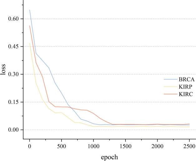
The variation of the loss value with epoch on MoAGL-SA
Comparison with previous methods
MoAGL-SA was compared with five classification methods that utilized multi-omics data including three classical methods i.e., k-nearest neighbor classifier (KNN), support vector machine classifier (SVM), random forest (RF), as well as two DL-based methods of MoGCN and MORONET.
KNN, the final classification was decided by voting of k-nearest neighbors;
SVM identified an optimal hyperplane that maximally separated the different classes of data set;
RF constructed multiple decision trees during training and output the class that was the mode of all the individual decision tree predictions;
MoGCN [14] is a multi-omics integration method for cancer subtype classification based on GCN, which used AE and SNF to reduce dimensionality and construct the patient similarity network respectively;
MORONET [13] is a method that jointly used GCN and VCDN for multi-omics data classification.
All competitive methods were implemented using publicly available code. The scikit-learn package was mainly used to implement these methods with default parameters. The input data of these classical methods was a single matrix that concatenated the multi-omics data. MoGCN, MORONET, and the proposed method were implemented using the PyTorch framework. MoGCN utilized AEs trained with mean squared error, followed by SNF for patient similarity network construction and a two-layer GCN. MORONET trained a three-layer GCN with L2 parametric loss, while VCDN was trained with cross-entropy loss. The critical threshold k, determining the average number of neighbors per sample, was set between 2 and 10.
Following the approach in [13], 70% of the samples were used for training, and the remaining 30% for testing. During testing, all samples were input to the model to maintain their relationships, and evaluation metrics were calculated only on the test set. The average evaluation metrics were calculated from five random runs. Additionally, computational time was reported to provide a comprehensive overview of performance efficiency. Table 2 displays the classification results on three datasets.
Table 2.
Comparison of different classification methods on the cancer datasets
| Method | BRCA | KIRP | KIRC | |||||||||
|---|---|---|---|---|---|---|---|---|---|---|---|---|
| ACC (%) | F1-w (%) | F1-m (%) | Time (s) | ACC (%) | F1 (%) | AUC (%) | Time (s) | ACC (%) | F1 (%) | AUC (%) | Time (s) | |
| KNN | 73.17 | 68.96 | 68.20 | 0.20 | 81.82 | 89.71 | 56.25 | 0.08 | 68.09 | 76.19 | 64.44 | 0.05 |
| SVM | 75.61 | 70.71 | 64.00 | 0.59 | 88.31 | 93.02 | 74.18 | 0.69 | 72.34 | 77.19 | 70.74 | 1.28 |
| RF | 78.78 | 75.12 | 64.90 | 1.59 | 89.61 | 93.55 | 81.92 | 1.11 | 72.34 | 77.24 | 70.67 | 1.33 |
| MoGCN | 84.23 | 85.18 | 79.30 | 41.60 | 79.22 | 70.04 | 82.54 | 22.73 | 57.45 | 41.92 | 50.52 | 32.86 |
| MORONET | 84.82 | 84.56 | 77.40 | 57.17 | 89.09 | 93.45 | 85.89 | 48.40 | 70.85 | 77.00 | 73.21 | 46.85 |
| MoAGL-SA | 88.22 | 88.05 | 83.83 | 76.90 | 90.13 | 93.81 | 92.03 | 56.55 | 72.34 | 77.02 | 76.22 | 56.57 |
Bold indicators the highest value of each evaluation metric
As shown in Table 2, MoAGL-SA outperformed the five compared methods in most classification tasks. Although RF and SVM produced slightly higher F1 scores on the KIRC dataset, MoAGL-SA achieved comparable ACC and superior AUC. Compared to the other two GCN-based methods(MoGCN and MORONET), MoAGL-SA demonstrated superior performance in all classification tasks, though at the cost of increased computational time due to the need for optimizing the sample relationship graph.
The method integrated three types of omics data of mRNA, DNA methylation, and miRNA. To demonstrate the necessity of integrating multiple omics data for classification, we compared the classification results of the method using multi-omics data and single-omics data. Fig. 4 gives the results.
Fig. 4.

Classification results between multi-omics data and single-omics data via MoAGL-SA
Figure 4 shows that MoAGL-SA consistently outperformed the method based on single-omics data, except for AUC in the KIRC classification task, where DNA and miRNA individually achieved higher performance. The performance of different omics varied across classification tasks. For example, mRNA performed best in BRCA classification, whereas miRNA outperformed mRNA in KIRP classification. These results underscore the importance of integrating multi-omics data for robust classification performance.
Ablation experiments
To further validate the robustness of the proposed method, ablation studies were systematically conducted, focusing on both key modules and key parameters.
To assess the effectiveness of the graph learning module, we replaced the graph learning module with a KNN and cosine distance-based graph construction method (denoted as Consine_n), where n (2,4,8,16) represents the number of k-nearest neighbors. Table 3 displays the results for MoAGL-SA compared to Consine_n. From Table 3, the following results are observed: firstly, for the fixed composition method Consine_n, the classification performance of the model is sensitive to the value n. For example, in BRCA classification task, the maximum and minimum values of ACC are obtained when n is set to 2 and 16 respectively. Secondly, compared with Consine_n methods, MoAGL-SA achieves superior performance across various classification metrics. This demonstrates the effectiveness of the graph learning module in constructing the sample similarly graph and yielding more accurate and robust classification results.
Table 3.
Ablation experiments of the graph learning module
| Method | BRCA | KIRP | KIRC | ||||||
|---|---|---|---|---|---|---|---|---|---|
| ACC (%) | F1-w (%) | F1-m (%) | ACC (%) | F1 (%) | AUC (%) | ACC (%) | F1 (%) | AUC (%) | |
| Consine_2 | 85.48 | 85.10 | 77.71 | 81.30 | 88.12 | 77.42 | 71.28 | 74.52 | 74.92 |
| Consine_4 | 82.99 | 82.71 | 71.32 | 84.67 | 90.52 | 82.85 | 70.43 | 73.26 | 73.28 |
| Consine_8 | 81.91 | 80.60 | 74.13 | 85.97 | 91.31 | 81.82 | 70.85 | 74.72 | 74.35 |
| Consine_16 | 81.49 | 81.14 | 76.23 | 81.56 | 88.62 | 83.26 | 69.79 | 73.77 | 73.16 |
| MoAGL-SA | 88.22 | 88.05 | 83.83 | 90.13 | 93.81 | 92.03 | 72.34 | 77.02 | 76.22 |
Bold indicators the highest value of each evaluation metric
In addition, to verify the effectiveness of SA module in omics integration, we replaced SA with two alternative methods, simply adding various omics features (GCN_NA) and assigning equal weights (GCN_EQU) to different omics. From Table 4, we can see that GCN_NA and GCN_EQU methods have a relatively low classification performance in most evaluation metrics for three cancers, which illustrates that ordinary integration strategy that directly adds various omics features or assigns equal weights for different omics may be insufficient for cancer subtype classification. This demonstrates the superiority of the SA-based integration module in enhancing MoAGL-SA’s ability to effectively distinguish cancer subtypes. Furthermore, the best classification performance is achieved by combining two key modules in the proposed method for three cancers, which demonstrates the superiority of graph learning for automatically constructing sample relationship graph and SA based adaptive integration modules for cancer subtype classification.
Table 4.
Ablation experiments of the omics integration module
| Method | BRCA | KIRP | KIRC | ||||||
|---|---|---|---|---|---|---|---|---|---|
| ACC (%) | F1-w (%) | F1-m (%) | ACC (%) | F1 (%) | AUC (%) | ACC (%) | F1 (%) | AUC (%) | |
| GCN_NA | 77.10 | 73.92 | 70.71 | 83.38 | 88.42 | 90.61 | 70.00 | 74.28 | 76.14 |
| GCN_EQU | 81.41 | 79.98 | 68.67 | 80.78 | 86.85 | 90.05 | 68.09 | 73.60 | 76.06 |
| MoAGL-SA | 88.22 | 88.05 | 83.83 | 90.13 | 93.81 | 92.03 | 72.34 | 77.02 | 76.22 |
Bold indicators the highest value of each evaluation metric
Further ablation experiments were conducted to evaluate the impact of the key parameters(, , , ). and are the coefficients for graph learning loss and omics reconstruction loss, respectively, which determine the importance of graph learning and omics reconstruction task. Ablation experiments were conducted where one parameter was fixed at while the other was set to [, , , , 0]. and are key parameters for graph learning loss, where controls the sparsity of the adjacency matrix and governs the importance of the samples. Similarly, the ablation experiment was set with these two parameters of 0.3 and 0.7, respectively, with one parameter unchanged in the solid state and the other set to [0.1, 0.3, 0.5, 0.7, 0.9]. Table 5 displays the results of the ablation results for the key parameters.
Table 5.
Ablation experiments of the key parameters
| Method | BRCA | KIRP | KIRC | ||||||
|---|---|---|---|---|---|---|---|---|---|
| ACC (%) | F1-w (%) | F1-m (%) | ACC (%) | F1 (%) | AUC (%) | ACC (%) | F1 (%) | AUC (%) | |
|
=, = |
81.78 | 77.18 | 67.99 | 85.30 | 85.90 | 83.32 | 57.45 | 72.97 | 71.48 |
|
=, = |
80.54 | 80.20 | 75.25 | 87.90 | 87.60 | 83.83 | 58.51 | 73.47 | 73.82 |
|
=, = |
80.12 | 76.73 | 70.16 | 79.22 | 88.41 | 89.27 | 62.77 | 74.82 | 73.36 |
|
=0, = |
70.12 | 65.91 | 56.41 | 79.22 | 80.41 | 76.66 | 53.19 | 66.15 | 65.62 |
|
=, = |
85.10 | 83.25 | 80.32 | 86.62 | 86.76 | 79.94 | 60.64 | 73.47 | 71.69 |
|
=, = |
87.18 | 85.36 | 82.39 | 89.22 | 88.41 | 80.30 | 69.57 | 74.48 | 74.68 |
|
=, = |
85.93 | 83.91 | 82.74 | 87.92 | 87.41 | 81.73 | 62.77 | 74.45 | 71.78 |
|
=, =0 |
81.37 | 76.27 | 67.18 | 80.52 | 88.89 | 79.68 | 60.64 | 72.97 | 67.95 |
|
=, = |
88.22 | 88.05 | 83.83 | 90.13 | 93.81 | 92.03 | 72.34 | 77.02 | 76.22 |
|
=0.1, =0.7 |
85.78 | 86.09 | 77.99 | 89.22 | 88.41 | 83.17 | 64.89 | 74.47 | 68.08 |
|
=0.5, =0.7 |
86.35 | 86.43 | 81.85 | 90.02 | 88.89 | 86.91 | 62.77 | 73.45 | 68.38 |
|
=0.7, =0.7 |
84.61 | 86.10 | 81.22 | 89.22 | 88.41 | 84.75 | 60.64 | 73.48 | 66.62 |
|
=0.9, =0.7 |
82.32 | 83.36 | 80.23 | 89.22 | 88.41 | 77.02 | 59.57 | 73.97 | 67.99 |
|
=0.3, =0.1 |
85.54 | 87.14 | 74.43 | 89.22 | 88.24 | 90.09 | 70.64 | 74.13 | 71.57 |
|
=0.3, =0.3 |
85.95 | 87.24 | 81.68 | 90.02 | 90.05 | 91.22 | 70.64 | 73.47 | 74.03 |
|
=0.3, =0.5 |
86.80 | 87.56 | 82.76 | 87.92 | 87.41 | 91.27 | 70.64 | 72.97 | 70.79 |
|
=0.3, =0.9 |
83.78 | 82.25 | 79.08 | 86.62 | 86.76 | 91.22 | 71.70 | 73.53 | 71.23 |
|
=0.3, =0.7 |
88.22 | 88.05 | 83.83 | 90.13 | 93.81 | 92.03 | 72.34 | 77.02 | 76.22 |
Bold indicators the highest value of each evaluation metric
It is observed that the optimal performance across all three datasets occurs when both and are set to 1e-3. This parameter setting demonstrates an effective balance, providing high accuracy and F1 scores, indicating that it optimally balances performance across different datasets. Notably, variations in have a more pronounced impact on model performance compared to changes in . This suggests that the graph learning task, relative to the omics reconstruction task, plays a more crucial role in influencing the final classification outcomes. Our model achieves the best performance under the setting =0.3 =0.7 compared with other settings. This further demonstrates the important role of graph learning tasks in the model. The above results show that appropriate parameter selection is the key to achieve robust and stable performance.
Case studies
To demonstrate the ability of MoAGL-SA in identifying cancer subtypes and enhance the interpretability of MoAGL-SA, the Permutation importance method [28] was applied for important feature ranking and selection on BRCA dataset whose subtype was more complex compared to the other two datasets. Firstly, the input data is normalized to the range of [0,1]. Next, randomly set one of the feature values to 0 in the test dataset and use the trained model to re-predict the dataset. The attenuation of model performance represents the importance of the feature. In the BRCA classification task, ACC is used to evaluate the attenuation of MoAGL-SA model’s performance. By repeating this process for all features, the feature importance calculation is completed and the feature with the most significant decrease is identified as the most critical feature. Table 6 displays the top 100 biomarkers for the BRCA dataset from mRNA expression data.
Table 6.
The top 100 biomarkers of BRCA dataset
| Rank | Gene | Rank | Gene | Rank | Gene | Rank | Gene |
|---|---|---|---|---|---|---|---|
| 1 | E2F8 | 26 | TCEAL7 | 51 | LRRFIP1 | 76 | CARKD |
| 2 | YBX2 | 27 | GRIN2A | 52 | SLITRK5 | 77 | PLAC9 |
| 3 | PRR11 | 28 | EPCAM | 53 | PRKCA | 78 | SLITRK6 |
| 4 | KIF20A | 29 | MAL2 | 54 | PBX2 | 79 | SOX5 |
| 5 | PRPH | 30 | ZG16 | 55 | ESYT1 | 80 | SLIT1 |
| 6 | DEPDC1B | 31 | MMP28 | 56 | C10orf58 | 81 | PHLDA2 |
| 7 | TFR2 | 32 | ZSCAN10 | 57 | PYY2 | 82 | ESAM |
| 8 | MYBL1 | 33 | IBSP | 58 | SLCO4C1 | 83 | CKMT1A |
| 9 | BTNL9 | 34 | NDRG4 | 59 | SPINK4 | 84 | CLDN18 |
| 10 | KCNG3 | 35 | FA2H | 60 | DRP2 | 85 | CKMT1B |
| 11 | BARD1 | 36 | PLD4 | 61 | PKHD1 | 86 | LRRC55 |
| 12 | VSTM1 | 37 | P2RY1 | 62 | ARHGEF7 | 87 | GPRASP1 |
| 13 | TREH | 38 | PAX2 | 63 | SLITRK3 | 88 | RDH16 |
| 14 | NEFL | 39 | SLC6A11 | 64 | DQX1 | 89 | CAMK1 |
| 15 | SOX17 | 40 | RPL39L | 65 | COX7A1 | 90 | ERBB2 |
| 16 | CDH1 | 41 | IP6K3 | 66 | SGCA | 91 | C9orf7 |
| 17 | psiTPTE22 | 42 | MYOM3 | 67 | TRIM29 | 92 | SPIN1 |
| 18 | TMEM59L | 43 | PYCR1 | 68 | CKMT2 | 93 | SSX4 |
| 19 | TRPM2 | 44 | APOBEC3B | 69 | PTGDS | 94 | GPR128 |
| 20 | PALMD | 45 | ANKRD26P1 | 70 | TARP | 95 | C8orf84 |
| 21 | LTBP2 | 46 | SLC5A11 | 71 | ST8SIA6 | 96 | UGT1A5 |
| 22 | FAM83A | 47 | CES3 | 72 | NRN1 | 97 | GDPD2 |
| 23 | RAB42 | 48 | PPP1R9A | 73 | XKR8 | 98 | RNF17 |
| 24 | NMU | 49 | SEPT5 | 74 | RABEPK | 99 | ADH1A |
| 25 | ME1 | 50 | SEMA6C | 75 | C6orf145 | 100 | APOA2 |
Several biomarkers identified by MoAGL-SA have known associations with breast cancer. For example, E2F8 demonstrated robust elevation in both breast cancer cell lines and clinical tissue samples. Studies by Ye et al. confirmed that upregulation of E2F8 significantly promoted breast cancer cell proliferation and tumorigenicity both in vitro and vivo [29]. KIF20A was more frequently expressed in human epidermal growth factor receptor 2 (HER2) -positive and triple-negative breast cancer than in the luminal type. Masako et al. [30] indicated that KIF20A expression was an independent prognostic factor for breast cancer. In addition, overexpression of tumor-related KIFs correlated with worse outcomes of breast cancer patients and could work as a potential prognostic biomarker [31]. Additionally, DEPDC1B was also demonstrated to be overexpressed in breast cancer [32].
Meanwhile, the biomarkers mentioned above also ranked high among differentially expressed genes in mRNA expression data, as shown in Table 7, which is sorted by false discovery rate (FDR). It validated the effectiveness of the proposed method in discovering these key biomarkers.
Table 7.
The top 10 differentially expressed genes in mRNA expression data of BRCA dataset
| Rank | Gene | FDR |
|---|---|---|
| 1 | DEPDC1B | 2.70E-22 |
| 2 | NAT1 | 3.81E-20 |
| 3 | E2F8 | 3.81E-20 |
| 4 | AGR3 | 4.63E-20 |
| 5 | KIF20A | 4.63E-20 |
| 6 | SCUBE2 | 5.38E-20 |
| 7 | ERBB4 | 5.38E-20 |
| 8 | TFF1 | 7.64E-20 |
| 9 | CA12 | 2.31E-19 |
| 10 | BCL11A | 2.74E-19 |
Bold indicates that this gene also appears among the top genes selected by MoAGL-SA
Furthermore, to demonstrate the relationship between identified biomarkers and breast cancer, KEGG pathway enrichment analyses and GO enrichment analyses, including biological process (BP) annotation, cellular component (CC) annotation, and molecular function (MF) annotation for the selected top 100 biomarkers, were conducted using DAVID (https://david.ncifcrf.gov/). The results of the enrichment analysis are shown in Fig. 5. The left subgraph of Fig. 5 shows the KEGG pathway enrichment analysis results, where the gene ratio refers to the pathway of biomarkers associated with a specific biological pathway or function related to the total number of biomarkers. A high gene ratio indicates that a significant portion of biomarkers is related to the pathway, suggesting a strong biological relevance. Conversely, a low gene ratio indicates a weaker association with a specific biological pathway. The right subgraph of Fig. 5 shows the GO enrichment analysis results. BP involves pathways and broader processes that the genes are involved in; CC pertains to the parts of the cell or extracellular environment where the genes are active; and MF describes the biochemical activities carried out by gene products.
Fig. 5.

The results of enrichment analysis on top 100 biomarkers
The KEGG pathway enrichment showed that these biomarkers were significantly enriched in the Metabolic pathways, Cell adhesion molecules, Pathways of neurodegeneration-multiple diseases, Arginine and proline metabolism, etc. Metabolic pathways of energy production and utilization were dysregulated in tumor cells, and this dysregulation was a newly accepted hallmark of cancer. Intervention measures on breast cancer pathways might benefit high-risk groups of breast cancer [33]. Cell adhesion molecules was considered essential for transducing intracellular signals responsible for adhesion, migration, invasion, angiogenesis, and organ-specific metastasis, which was related to the metastasis of breast cancer [34]. The GO enrichment analysis of the top 100 biomarkers showed that their biological function focused on the phosphocreatine biosynthetic process, axonogenesis, plasma membrane, basolateral plasma membrane, creatine kinase activity, and kinase activity. Cancer-related axonogenesis and neurogenesis were regarded as a novel biological phenomenon, and spatial and temporal associations between increased nerve density and preneoplastic and neoplastic lesions of the human prostate were identified [35], indicating that these biological phenomena might also be related to breast cancer, which deserves future research. In the aspect of the plasma membrane, the fourier transform infra-red spectra of plasma membrane proteins showed significant differences between normal and benign tissues compared to malignant tissues of breast cancer at 1536 and 1645 [36]. Although there is no direct literature to prove that the remaining biomarkers are related to breast cancer subtypes, the enrichment analysis results show that some biomarkers are involved in metabolic pathways, molecular functions, cellular components and biological processes that may be related to the development and progression of breast cancer. These findings provide a promising way for future research.
Discussion
This paper proposes MoAGL-SA, a novel multi-omics integration method combining graph learning, GCN, and SA in a unified framework. The graph learning of MoAGL-SA could adaptively construct sample relationship graph from each omics data, overcoming the limitations of traditional graph construction methods that required prior knowledge or manual operations. The SA-based multi-omics integration module automatically assigns weights to each omic, producing a final integrated feature representation.
Our experimental results on BRCA, KIRP, and KIRC demonstrate the superior classification performance of MoAGL-SA compared to classical methods and state-of-the-art DL-based methods. One important observation is that DL-based methods like MoGCN and MORONET did not consistently outperform classical methods on certain datasets. This may be due to the fact that MoGCN relies on AEs for feature extraction, which can be suboptimal for handling high-dimensional omics data, particularly for the KIRP and KIRC datasets. Additionally, MORONET, while effective for multi-class classification, appears less suited for binary classification tasks, which might explain its lower performance. However, MoAGL-SA consistently achieved superior results across multiple metrics. Its end-to-end learning approach, coupled with adaptive multi-omics integration, allowed it to handle complex data relationships more effectively, demonstrating its advantage over both classical and DL-based methods.
Our case studies on BRCA demonstrate MoAGL-SA’s capacity to identify biologically relevant biomarkers associated with breast cancer subtypes, such as E2F8, KIF20A, and DEPDC1B. The KEGG and GO enrichment analyses further validated the biological relevance of these biomarkers, highlighting their roles in processes like cell adhesion and metabolic pathways, which are known to be involved in cancer development.
Despite its promising results, MoAGL-SA has several limitations. First, the model requires complete multi-omics data, limiting its use in cases with missing data. Future work will explore imputation techniques or models that handle incomplete datasets. Second, while MoAGL-SA performed well on BRCA, KIRP, and KIRC datasets, its generalizability to other cancers remains to be evaluated, requiring validation on independent datasets. Lastly, although the model identified potential biomarkers, further clinical trials are needed to confirm their biological significance and relevance to cancer subtypes. Addressing these limitations will be the focus of future research.
Conclusion
In this study, we propose MoAGL-SA, an advanced multi-omics integration framework that combines graph learning, GCNs, and self-attention to enhance cancer subtype classification. By automatically constructing sample relationship graphs and adaptively weighting each omics, MoAGL-SA not only achieves outstanding classification accuracy but also effectively identifies biologically relevant biomarkers. Its adaptive, end-to-end design outperforms classical and DL-based methods, providing a promising tool for advancing precision medicine through flexible multi-omics integration.
Author contributions
P.G. conceived the project. P.G., L.C., Q.H., and Y.L. designed and implemented the algorithms and models. L.C., S.G., Z.Z. and L.Z. analyzed and interpreted the data. P.G. and L.C. drafted the manuscript. All authors approved the final article. All authors have read and agreed to the published version of the manuscript.
Funding
This work was supported by the Natural Science Foundation of China (No. 82001987), the Postgraduate Research & Practice Innovation Program of Jiangsu Province (No.KYCX23_2937), and the Innovation and Entrepreneurship Project of Xuzhou Medical University Science Park (No. CXCYZX2022010).
Availability of data and materials
BRCA, KIRP and KIRC datasets were available in the TCGA ( https://portal.gdc.cancer.gov/). MoAGL-SA is implemented in Python and is available on GitHub (https://github.com/gpxzmu/MoAGL-SA)
Declarations
Ethics approval and consent to participate
Not applicable.
Consent for publication
Not applicable.
Competing interests
Not applicable.
Footnotes
Publisher's Note
Springer Nature remains neutral with regard to jurisdictional claims in published maps and institutional affiliations.
References
- 1.Tan K, Huang W, Hu J, Dong S. A multi-omics supervised autoencoder for pan-cancer clinical outcome endpoints prediction. BMC Med Inform Decis Mak. 2020;20:1–9. [DOI] [PMC free article] [PubMed] [Google Scholar]
- 2.Tomczak K, Czerwińska P, Wiznerowicz M. Review the cancer genome atlas (TCGA): an immeasurable source of knowledge. Contemp Oncol/Współcz Onkol. 2015;2015(1):68–77. [DOI] [PMC free article] [PubMed] [Google Scholar]
- 3.Günther OP, Chen V, Freue GC, Balshaw RF, Tebbutt SJ, Hollander Z, Takhar M, McMaster WR, McManus BM, Keown PA, et al. A computational pipeline for the development of multi-marker bio-signature panels and ensemble classifiers. BMC Bioinform. 2012;13(1):1–18. [DOI] [PMC free article] [PubMed] [Google Scholar]
- 4.Kim D, Li R, Dudek SM, Ritchie MD. Athena: identifying interactions between different levels of genomic data associated with cancer clinical outcomes using grammatical evolution neural network. BioData Mining. 2013;6(1):1–14. [DOI] [PMC free article] [PubMed] [Google Scholar]
- 5.Singh A, Shannon CP, Gautier B, Rohart F, Vacher M, Tebbutt SJ, Lê Cao K-A. Diablo: an integrative approach for identifying key molecular drivers from multi-omics assays. Bioinformatics. 2019;35(17):3055–62. [DOI] [PMC free article] [PubMed] [Google Scholar]
- 6.Li J, Xie L, Xie Y, Wang F. Bregmannian consensus clustering for cancer subtypes analysis. Comput Methods Programs Biomed. 2020;189: 105337. [DOI] [PubMed] [Google Scholar]
- 7.Menyhárt O, Győrffy B. Multi-omics approaches in cancer research with applications in tumor subtyping, prognosis, and diagnosis. Comput Struct Biotechnol J. 2021;19:949–60. [DOI] [PMC free article] [PubMed] [Google Scholar]
- 8.Huang Z, Zhan X, Xiang S, Johnson TS, Helm B, Yu CY, Zhang J, Salama P, Rizkalla M, Han Z, et al. Salmon: survival analysis learning with multi-omics neural networks on breast cancer. Front Genet. 2019;10:166. [DOI] [PMC free article] [PubMed] [Google Scholar]
- 9.Yang H, Chen R, Li D, Wang Z. Subtype-GAN: a deep learning approach for integrative cancer subtyping of multi-omics data. Bioinformatics. 2021;37(16):2231–7. [DOI] [PubMed] [Google Scholar]
- 10.Zhao L, Dong Q, Luo C, Wu Y, Bu D, Qi X, Luo Y, Zhao Y. Deepomix: A scalable and interpretable multi-omics deep learning framework and application in cancer survival analysis. Comput Struct Biotechnol J. 2021;19:2719–25. [DOI] [PMC free article] [PubMed] [Google Scholar]
- 11.Kipf TN, Welling M. Semi-supervised classification with graph convolutional networks. arXiv preprint arXiv:1609.02907 2016.
- 12.Sun F, Sun J, Zhao Q. A deep learning method for predicting metabolite-disease associations via graph neural network. Brief Bioinform. 2022;23(4):266. [DOI] [PubMed] [Google Scholar]
- 13.Wang T, Shao W, Huang Z, Tang H, Zhang J, Ding Z, Huang K. Moronet: multi-omics integration via graph convolutional networks for biomedical data classification. bioRxiv, 2020–07 2020.
- 14.Li X, Ma J, Leng L, Han M, Li M, He F, Zhu Y. MOGCN: a multi-omics integration method based on graph convolutional network for cancer subtype analysis. Front Genet. 2022;13: 806842. [DOI] [PMC free article] [PubMed] [Google Scholar]
- 15.Yang B, Yang Y, Wang M, Su X. MRGCN: cancer subtyping with multi-reconstruction graph convolutional network using full and partial multi-omics dataset. Bioinformatics. 2023;39(6):353. [DOI] [PMC free article] [PubMed] [Google Scholar]
- 16.Vaswani A, Shazeer N, Parmar N, Uszkoreit J, Jones L, Gomez AN, Kaiser Ł, Polosukhin I. Attention is all you need. Adv Neural Inform Process Syst. 2017. 10.48550/arXiv.1706.03762. [Google Scholar]
- 17.Xu P, Zhu X, Clifton DA. Multimodal learning with transformers: A survey. IEEE Trans Pattern Anal Mach Intell. 2023;45(10):12113–32. [DOI] [PubMed] [Google Scholar]
- 18.Luong M-T, Pham H, Manning CD. Effective approaches to attention-based neural machine translation. arXiv preprint arXiv:1508.04025 2015.
- 19.Khattar D, Kumar V, Varma V, Gupta M. Hram: A hybrid recurrent attention machine for news recommendation. In: Proceedings of the 27th ACM international conference on information and knowledge management; 2018. p. 1619–22.
- 20.Mnih V, Heess N, Graves A, et al. Recurrent models of visual attention. Adv Neural Inform Process Syst. 2014;27.
- 21.Srivastava P, Bej S, Yordanova K, Wolkenhauer O. Self-attention-based models for the extraction of molecular interactions from biological texts. Biomolecules. 2021;11(11):1591. [DOI] [PMC free article] [PubMed] [Google Scholar]
- 22.Ma B, Meng F, Yan G, Yan H, Chai B, Song F. Diagnostic classification of cancers using extreme gradient boosting algorithm and multi-omics data. Comput Biol Med. 2020;121: 103761. [DOI] [PubMed] [Google Scholar]
- 23.Liu X, Gao F, Zhang Q, Zhao H. Graph convolution for multimodal information extraction from visually rich documents. arXiv preprint arXiv:1903.11279 .2019
- 24.Yu W, Lu N, Qi X, Gong P, Xiao R. Pick: processing key information extraction from documents using improved graph learning-convolutional networks. In: 2020 25th International conference on pattern recognition (ICPR); 2021. p. 4363–70. IEEE.
- 25.Ouyang D, Liang Y, Li L, Ai N, Lu S, Yu M, Liu X, Xie S. Integration of multi-omics data using adaptive graph learning and attention mechanism for patient classification and biomarker identification. Comput Biol Med. 2023;164: 107303. [DOI] [PubMed] [Google Scholar]
- 26.Jiang B, Zhang Z, Lin D, Tang J, Luo B. Semi-supervised learning with graph learning-convolutional networks. In: Proceedings of the IEEE/CVF conference on computer vision and pattern recognition; 2019. p. 11313–20.
- 27.Huang H, Song Y, Wu Y, Shi J, Xie X, Jin H. Multitask representation learning with multiview graph convolutional networks. IEEE Trans Neural Netw Learn Syst. 2020;33(3):983–95. [DOI] [PubMed] [Google Scholar]
- 28.Fisher A, Rudin C, Dominici F. All models are wrong, but many are useful: Learning a variable’s importance by studying an entire class of prediction models simultaneously. J Mach Learn Res. 2019;20(177):1–81. [PMC free article] [PubMed] [Google Scholar]
- 29.Ye L, Guo L, He Z, Wang X, Lin C, Zhang X, Wu S, Bao Y, Yang Q, Song L, et al. Upregulation of E2F8 promotes cell proliferation and tumorigenicity in breast cancer by modulating G1/S phase transition. Oncotarget. 2016;7(17):23757. [DOI] [PMC free article] [PubMed] [Google Scholar]
- 30.Nakamura M, Takano A, Thang PM, Tsevegjav B, Zhu M, Yokose T, Yamashita T, Miyagi Y, Daigo Y. Characterization of KIF20A as a prognostic biomarker and therapeutic target for different subtypes of breast cancer. Int J Oncol. 2020;57(1):277–88. [DOI] [PubMed] [Google Scholar]
- 31.Li T-F, Zeng H-J, Shan Z, Ye R-Y, Cheang T-Y, Zhang Y-J, Lu S-H, Zhang Q, Shao N, Lin Y. Overexpression of kinesin superfamily members as prognostic biomarkers of breast cancer. Cancer Cell Int. 2020;20:1–16. [DOI] [PMC free article] [PubMed] [Google Scholar]
- 32.Boudreau HE, Broustas CG, Gokhale PC, Kumar D, Mewani RR, Rone JD, Haddad BR, Kasid U. Expression of BRCC3, a novel cell cycle regulated molecule, is associated with increased phospho-ERK and cell proliferation. Int J Mol Med. 2007;19(1):29–39. [PubMed] [Google Scholar]
- 33.Brown KA. Metabolic pathways in obesity-related breast cancer. Nat Rev Endocrinol. 2021;17(6):350–63. [DOI] [PMC free article] [PubMed] [Google Scholar]
- 34.Li D-M, Feng Y-M. Signaling mechanism of cell adhesion molecules in breast cancer metastasis: potential therapeutic targets. Breast Cancer Res Treat. 2011;128:7–21. [DOI] [PubMed] [Google Scholar]
- 35.Ayala GE, Dai H, Powell M, Li R, Ding Y, Wheeler TM, Shine D, Kadmon D, Thompson T, Miles BJ, et al. Cancer-related axonogenesis and neurogenesis in prostate cancer. Clin Cancer Res. 2008;14(23):7593–603. [DOI] [PubMed] [Google Scholar]
- 36.Fahmy HM, Ismail AM, El-Feky AS, Serea ESA. Elshemey WM Plasma membrane proteins: A new probe for the characterization of breast cancer. Life Sci. 2019;234: 116777. [DOI] [PubMed] [Google Scholar]
Associated Data
This section collects any data citations, data availability statements, or supplementary materials included in this article.
Data Availability Statement
BRCA, KIRP and KIRC datasets were available in the TCGA ( https://portal.gdc.cancer.gov/). MoAGL-SA is implemented in Python and is available on GitHub (https://github.com/gpxzmu/MoAGL-SA)