Can Deep Learning Search for Exceptional Chiroptical Properties? The Halogenated [6]Helicene Case

Abstract

The relationship between chemical structure and chiroptical properties is not always clearly understood. Nowadays, efforts to develop new systems with enhanced optical properties follow the trial‐error method. A large number of data would allow us to obtain more robust conclusions and guide research toward molecules with practical applications. In this sense, in this work we predict the chiroptical properties of millions of halogenated [6]helicenes in terms of the rotatory strength (R). We have used DFT calculations to randomly create derivatives including from 1 to 16 halogen atoms, that were then used as a data set to train different deep neural network models. These models allow us to i) predict the R_max for any halogenated [6]helicene with a very low computational cost, and ii) to understand the physical reasons that favour some substitutions over others. Finally, we synthesized derivatives with higher predicted R _max obtaining excellent correlation among the values obtained experimentally and the predicted ones.

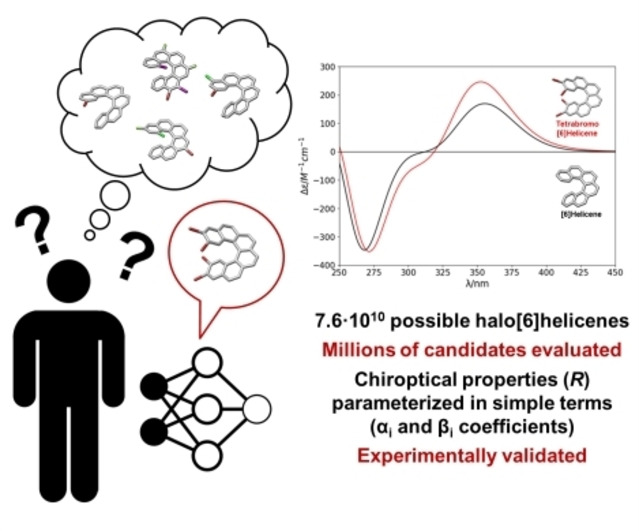
In this work, we have focused on one of the most important chiral motifs, [6]helicene, and we have predicted the effect of halogenation on its chiroptical properties using Deep Learning. We have developed three machine learning models, which allow us to evaluate millions of compounds and learn the reasons that favor some substitutions. With the knowledge gained, we synthesized the most favored candidates, exhibiting the predicted properties.

Introduction

[n]Helicenes are prototypical helical structures consisting of n ortho‐fused phenyl rings.[ ¹ , ² , ³ ] They also present high racemization barriers (when n>5) and show interesting chiroptical properties.[ ⁴ , ⁵ ] Remarkably, such properties can be now predicted with high confidence using DFT calculations with relatively low computational cost for the smallest members of the family.[ ⁶ , ⁷ , ⁸ , ⁹ , ¹⁰ ] However, although the chiroptical properties are codified in the intrinsic physics of the molecule, it is not easy to extract any structure–property relationship (apart from absolute configuration) from such kind of calculations. Even in the case that any correlation would exist, a huge volume of examples or data should be necessary for its understanding. The situation becomes more complex if we consider substitutions in the [n]helicene core. As an example, if we consider multiple halogen substitution in any of the sixteen positions in [6]helicene (Figure 1a), the challenge is intimidating. Eq. 1 gives the number of different compounds that can be obtained with k substituents also considering the rotation symmetry dividing the general expression by 2.

$${\displaystyle N_k=\frac{1}{2}\left(\begin{array}{c}16\\ k\end{array}\right)4^k}$$ (1)

$${\displaystyle N_1=32N_2=960N_3=17920}$$

$${\displaystyle N_4\approx 2.3x{10}^5{N}_5\approx 2.2x{10}^6{N}_6\approx 1.6x{10}^7}$$

Figure 1.

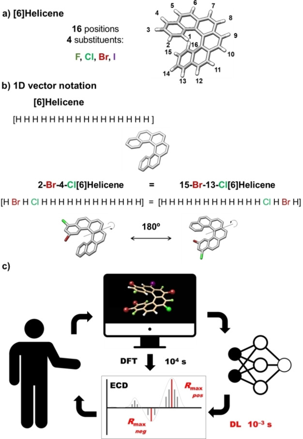
a) [6]helicene structure. Geometry optimized at the M06/TZVP level of calculation (PCM dichloromethane). b) 1D vector notation examples employed for differently halogenated [6]helicenes. c) Interplay between DFT calculations and Deep Learning (DL) based training and prediction of chiroptical properties.

Thus, if we consider the mono‐halogenation case only 32 derivatives can exist. An additional halogen rise the possibilities to 960, being the DFT calculations costly but affordable in a reasonable period whereas the in‐depth analysis of the resulting data begins to be daunting. Including four halogens increase the number of structures to almost 2.33×10⁵ and for hexadecahalogenated [6]helicenes the variation gives an astonishing number of 2.15×10⁹ different compounds. In those cases, neither theoretical calculations nor the analysis becomes viable. Globally, considering from mono‐ to hexadeca‐halogenated [6]helicenes, 7.63×10¹⁰ structures should be evaluated.

The problem is even more complex considering that chiroptical properties are diverse and the corresponding magnitude of the response can be defined in many ways. In this work we have focused our attention on electronic circular dichroism (ECD), one of the prototypical chiroptical techniques employed. ^[6] In this case, rotational strength (R_0j ), which is associated with each ground to excited state transition (0 to j), is a good indicator. ^[11] This scalar represents the intensity of the chiroptical response and a complete set of R_0j values can be extracted from theoretical calculations (Figure 1c). Thus, the shape of the ECD spectra is mainly constituted of the most intense transitions which in turn represent higher values of R_0j .

Considering the above‐mentioned framework, giving an answer to the question, “what is the maximum value for a rotatory strength in a (poly)halogenated [6]helicene?”, is daunting for standard approaches. As an alternative, machine learning (ML) techniques have succeeded in many cases to extract hidden patterns and develop predictions for complex problems only from data points of the observed phenomenon. ^[12] Specifically, neural networks – the computational model behind deep learning – have shown efficiency in Chemistry[ ¹³ , ¹⁴ , ¹⁵ ] as to optimize ^[16] and classify organic reaction mechanisms,[ ¹⁷ , ¹⁸ , ¹⁹ , ²⁰ , ²¹ , ²² , ²³ , ²⁴ ] predict molecular properties[ ²⁵ , ²⁶ , ²⁷ , ²⁸ , ²⁹ , ³⁰ , ³¹ , ³² ] and antibacterial activities. ^[33] Furthermore, the integration of machine learning and computational chemistry has proven to be very promising and fruitful,[ ³⁴ , ³⁵ , ³⁶ ] with applications such as developing[ ³⁷ , ³⁸ ] and accelerating DFT calculations[ ³⁹ , ⁴⁰ ] or the development of potentials to model chemical processes in solution. ^[41] Indeed, despite ML methodologies have been applied to achiral nanomaterials, there are no examples including chirality. ^[42] It is also worth noting that the models applied to the search of new materials with improved properties must meet two important requirements: i) to be able to extrapolate values for the extreme cases, where exceptional materials are, and ii) to propose synthetically viable candidates. ^[43] Within this context, we tackled the starting point question using DL approaches, searching for exceptional responses. We have focused on chiroptical properties of [6]helicene, one of the most significant chiral motifs. These systems have been proposed as promising candidates for chiroptical responses and their applications in devices,[ ⁴⁴ , ⁴⁵ , ⁴⁶ , ⁴⁷ ] making their study valuable beyond pure scientific curiosity and the pursuit of fundamental knowledge. A key aspect of our approach is the ability to predict chiroptical properties in [6]helicenes more rapidly than traditional methods, such as DFT simulations. This enables for the efficient estimation of maximum R _0j values (R _max) across a large number of systems (Figure 1c). With millions of data points available, robust patterns and conclusions can be established. Therefore, we aimed to determine if there is a limit to R _max and, if so, what it is. Thus, knowing the limit, we can either be driven to explore these limits or, on the other hand, we can turn to other chiral entities. Here we have designed and trained a neural network able to estimate R_max of halogenated [6]helicenes with a minimal computational cost, affording structure–property relationships for systems ranging from mono‐ to hexadeca‐halogenated [6]helicenes (Figure 1a). Such results were then compared with the prediction of two simpler and physically interpretable models. In these models, R_max values can be deconvoluted as a linear combination of coefficients depending on the relative position of 1 to 2 halogens on the structure. While the approach is less precise than DFT calculations, the developed models allow a rationalization of the results by two main reasons: i) the neural network can produce a big amount of data that additionally fits with those obtained through calculations and ii) simpler models give interpretable physical information of the behaviour of the system. The former allows the creation of a full database in which the selection of the better substitution pattern is straightforward even for blind interpretative models. Considering the latter, we have interestingly found that better values correspond to certain structures, indicating that some positions and atoms are preferred. Under this circumstance, a kind of parameterization can be made, assigning different weights to each halogen for each position. This situation resembles the concept of free energy linear relationships developed from seminal studies by Hammet. ^[48] That is, primary positions of the halogens establish a relative weight, α_i coefficients, using hydrogen atom substitution as a reference. Vicinal substitutions are then considered as secondary corrections, quantified in β_i coefficients.

We have organized the discussion presenting sequential training of models (up to hexahalogenated [6]helicenes) for which parameterizations seem to be robust, allowing a confident prediction about R_max . For highly substituted systems, the model has been statistically checked. The models determine that the best response in terms of R_max can be found for some tetra‐substituted [6]helicenes among thousands of millions of potential structures. Our full analysis suggests that 2,3,14,15‐tetrabromo [6]helicene 1 is the best candidate to achieve the highest rotatory strength. It is worth noting that R_max value for this compound has been predicted, being outside of the training dataset. The product has been synthesized and its chiroptical properties were experimentally determined, being in excellent agreement with the prediction.

Results and Discussion

Data Set and Model Training

The success of deep learning approaches relies on the capabilities of neural networks to approximate functions from several sample points. Thus, we decided to use data samples as pairs <X, Y>, where X is the representation of the molecule and Y is the property to be predicted (in this case R_max ) for a given X. Since all the input molecules share the same carbo[6]helicene skeleton, we decided to represent the helicene as a 1D vector constituted by 16 elements representing the substitution of the molecule (Figure 1b). To this regard, the combination of a simple vector containing the hydrogen position to be exchanged (1 to 16) and the nature of the saturation atom (0=H, 1=F, 2=Cl, 3=Br, and 4=I) is sufficient for a complete description of the structure. Furthermore, all models were built to respect the rotational symmetry of the molecule, being the position n equivalent to the position 17‐n, with n=1,…,16 (Figure 1b).

Despite the simplicity of the representation, all hidden contributions of any geometrical distortions (bond lengthening, resonance/inductive effects, etc) are codified in the calculated rotatory strengths. For the training, examples dealing only with the P configuration in the helix were selected. By symmetry, the conclusions of this study can be applied to the opposite M helical configuration. At this point, it is worth noting that R_0j values can be positive and negative and we have analysed both situations independently. The model is then trained to fit Y for X, and to make a meaningful estimation of Y for a given X. To this end, it is desirable to train the neural network with the most diverse and accurate available data. Hereof, theoretical calculations of a randomly selected family of [6]helicenes provided the dataset, including molecules with low and high R_max values.[ ³⁹ , ⁴⁹ ] It should also be noted that all the results are indispensable in every machine learning protocol.[ ⁵⁰ , ⁵¹ ]

Although neural networks are suitable regressors to capture complex non‐linear relations between input molecular representations and target magnitudes, they are black‐box models that suffer from a lack of interpretability. Therefore, we decided to accompany this approach with the 1‐ and 2‐body models, two simpler alternatives where the interpretation of the underlying physics is more easily achieved. In the simplest 1‐body model, the R_max of a molecule can be obtained directly by adding 16 α_i parameters to constant R_o . Those α_i coefficients (red in Figure 2) simply evaluate which substituents are in the [6]helicene and in which position (e.g., in 1‐bromo[6]helicene there is a bromine in the position 1 and hydrogens in the rest). The 1‐body model was defined by a 1D vector, containing 5×8=40 free α_i parameters, coming from the number of different atoms (hydrogen plus four halogens) multiplied by the number of non‐equivalent positions (Figure 2a–3a and Eq. 2). That model is extremely simple in concept but allows for a very simple and understandable parametrization in terms of a few α_i coefficients. Furthermore, the 2‐body model is defined by a 5×5 matrix (Eq. 3) increasing the free parameters up to 240. It considers the previous α_i coefficient plus an additional contribution called β_i accounting for adjacent interactions between first neighbors (Figure 2b, Eq. 3). From such local and neighboring parameters, general conclusions can be drawn about the physics of the system. Following this terminology, the neural network model could be considered a many‐body model, hereafter called N‐body model (Figure 2c, Eq. 4), where the contributions of single positions are mixed by a multilayer perceptron (MLP) to obtain the final output (Figure 3b). Obviously, the accuracy of the N‐body neural network model, with 9257 parameters, is better than that of the 1‐ and 2‐body models. However, the possibility of easily parameterizing the response together with the good correlations also obtained from simpler models, makes them very attractive and powerful strategies. All models have an adding constant (R ₀), which is set to the mean rotatory strength of the whole dataset.

Figure 2.

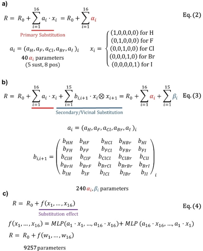
Equations and parameters for (a) 1‐body, (b) 2‐body and (c) N‐body model where f is a neural network‐based function constructed to impose the symmetry.

Figure 3.

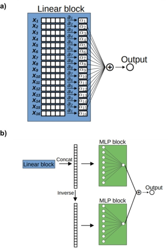
Process diagram of a) 1‐body and b) N‐body model.

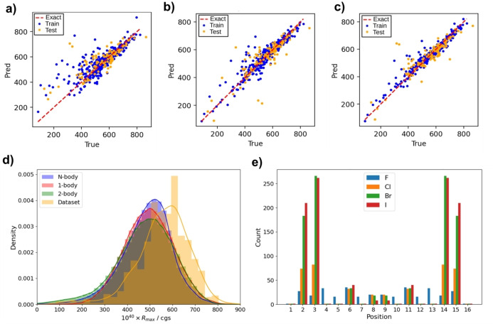
Our dataset was composed of 32 mono‐halogenated [6]helicenes and randomly selected families of di (150), tri (200), tetra (200), penta (200) and hexa‐halogenated [6]helicenes (400), constituting 1182 examples in total. For each molecule, the ECD spectra as a set of R_0j values versus absorption wavelengths were calculated using DFT methods as implemented in Gaussian 09 (see SI). ^[52] All R_max values given in the text are in 10⁻⁴⁰ cgs units. Most calculated positive R_max values are around 400–700 with minor subsets with examples presenting lower (100–300) and higher (800–900) ones (Figure 4d). Negative R_max values present a mean absolute value of −250 (R ₀) with a very minor subset beyond −600. Owing to this different behaviour we analysed the two scenarios independently. The dataset was then split into 80 % of the molecules for training and 20 % for testing. The robustness of the predictive models was tested by means of a 10‐times repeated random sub‐sampling validation. All the models were implemented and trained using TensorFlow. ^[53] A detailed explanation of the models, including the architecture of the neural network, the optimization of hyperparameters, and the training process, is provided in Section 2 of the Supporting Information. All scripts used for training the models, along with the complete dataset, are available in the repository https://github.com/alfonsogijon/Helicenes NNs. The prediction of R _max is treated as a regression task, and we employed evaluation metrics such as Mean Absolute Error (MAE), Mean Absolute Percentage (MAPE), Mean Squared Error (MSE) and coefficient of determination R², to assess the performance of the proposed methods. ^[54]

Figure 4.

Correlation between model‐predicted (y axis) vs DFT‐calculated (x axis) rotational strength values (R, 10⁻⁴⁰ cgs units) for halo[6]helicenes up to 4 halogen atoms (N=582 [6]helicenes) employing a) 1‐body, b) 2‐body, c) N‐body models. The statistical parameters of the models can be found in Table S1. d) Distributions of positive R_max obtained from DFT, 1‐, 2‐, and N‐body models for tetrahalogenated[6]helicenes. e) Location of halogens in molecules with high R _max from N‐body model for tetrahalogenated[6]helicenes.

Case 1. Positive R_max values for tetrahalogenated (P)‐[6]helicenes

The number of potential tetrahalogenated [6]helicenes is 232960, a number big enough to evaluate the feasibility of the DL approach. A set of 582 individual DFT calculations was used as training and test dataset. Figure 4 shows the correlation results using the three models, expanding from very different R_max values. The correlation improves with the number of bodies together with a decrease of data dispersion. In this sense, the N‐body model also presents a reasonable MAE of 17 and 30 10⁻⁴⁰ cgs for the train and test datasets, respectively (Figure 4c, Table S1). The MAE remains similar independently of the substitution degree which also evidences the reliability of the model (Figure S7). With the confidence that the model is suitable at this level of substitution, we then estimated the rest of the members of the tetrahalogenated family (Figure 4d). The prediction yielded an R_max distribution very similar to that obtained with the pure DFT dataset (Figure 4d, orange), spanning mainly from 200 to 800. Remarkably, the DFT‐calculated R_max value for the parent [6]helicene is 698 and the predicted one 696. These results suggest that the N‐body model is getting the underlying physics of the system. To achieve a better understanding of the origin of the R_max values, we analysed derivatives with R_max >800, finding a substantial preference (between 650 and 750 possibilities) when bromine and iodine atoms (Figure 4e, green and red bars respectively) are placed in the 2,3,14 and 15 positions. This intriguing preference for some positions and specific halogens could be rationalized simplifying the model and invoking a kind of parameterization. That is, the R_max value could be obtained by simple addition of individual contributions of substituents (α_i) to an initial R₀ value (Figure 2). Not surprisingly, the use of the 1‐body approach and the original N‐body simulation look similar (Figure 4d, blue and red), pointing out that the position, halogen, and R_max value are in fact closely related in an apparently systematic way. Thus, the extracted parameterization data (See Table 1) are relevant for rationalizing the previous findings obtained at the level of the N‐body model. Hydrogen substitution by a halogen generally disfavors the maximum R _max value except in the 2,3,14 and 15 positions when a bromine or iodine atom is placed. Nevertheless, spatially close 1,4,13 and 16 positions are compellingly highly disfavoring. In any case, 1‐body simulations must be only used to look for tendencies owing to the predicted R _max values are systematically higher than DFT ones. In addition, it is worth noting that the model is able to extrapolate values beyond those used in the training data set, which is of critical importance for our purpose. In this sense, 1‐Body model showed 15 privileged candidates for high R _max values (878 – 914) (Table S12), all of them possessing bromine and iodine atoms in the 2,3,14 and 15 positions. Their DFT R_max values were then calculated and it is especially relevant the case of 2,3,14,15‐tetrabromo [6]helicene 1 (Figure 5), with a DFT‐calculated R _max value of 942, astonishing for a small molecule.

Table 1.

α_i coefficients for with the 1‐body model

Position[a]	H[b]	F	Cl	Br[b]	I[b]
1	35.66	‐90.05	‐81.33	‐55.88	‐7.11
2	‐21.49	‐52.21	6.91	42.68	41.32
3	‐23.53	‐25.70	4.88	25.39	26.16
4	28.73	6.98	‐21.90	‐26.65	‐102.83
5	32.47	2.77	‐49.25	‐58.93	‐96.61
6	16.09	‐16.64	‐27.80	‐24.26	‐62.44
7	14.41	‐7.56	‐29.08	‐46.16	‐73.10
8	6.89	‐14.32	‐23.95	‐26.53	‐35.49

[a] n position is equivalent to 17‐n position (e.g. position 3 and position 14). [b] Green shading corresponds to the most favouring and red shading to the worst substitution. R₀ =508.89x10⁻⁴⁰ cgs units.

Figure 5.

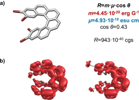
a) Structure of 2,3,14,15‐tetrabromo[6]helicene 1. b) Transition magnetic dipole moment density map for the best substitutions, corresponding to (2,15−) and (3,14−)dibromo [6]helicene.

Differences between 1‐ and N‐body simulations probably arise from the inability of the simplest model to describe secondary interactions between bulky halogens placed in contiguous positions. Thus, we built an improved 2‐body model including such contributions, quantified in β_i (Figure 4a‐b). The primary parameterization table (Table S3) remains similar to the previous one and secondary contributions correct the initial values using a new 5x5 matrix for each position (Tables S4–S11). A close inspection of the secondary corrections reveals that very few combinations can increase R_max because the global value is controlled by the primary parameterization. General trends show again that hydrogen atoms are the most efficient substituents for high R_max values, except for 2,3,14 and 15 positions in which bromine and iodine atoms are the best ones. An increase in the number of halogens is always detrimental to achieve high R values.

Trying to rationalize the results from a photophysical perspective, we analysed in more detail some prototypical examples. Symmetric structures with two halogens (1,16‐, 2,15‐, 3,14‐, … Figure S8) were calculated by DFT to find any potential structure–property relationship. R_0j is described as the scalar product of the electric (μ_0j ) and magnetic (m_0j ) transition dipole moments for a certain transition, R_0j =μ_0jm_0j =|μ_0j |⋅|m_0j |⋅cosθ. The corresponding parameters for dibrominated [6]helicenes and the parent [6]helicene are presented in Table 2. As can be seen, the best R_max values come from an optimization of both |m_0j | and θ. The value of |m_0j | is maximized when the transition involves the extended helicene π‐orbitals. ^[55] The visualization of the transition magnetic dipole moment density graphs employing the Multiwfn software package ^[56] displayed that the magnetic transition extends to the bromine atoms for some favoured (2,15 and 3,14) positions, thus creating a better electron circulation during the transition (Figure 5b), and enhancing |m| and R_max as a consequence. A similar analysis can be done for the iodine substitution (See Table S16). On the other hand, in compounds with fluorine and chlorine substitution |m| is not improved and the angle is also worse than the one in parent helicene (Tables S13–S14). Consequently, such substitutions are detrimental for exceptional R_max values. In essence, the privileged role of bromine and iodine in positions 2 and 3 can be rationalized on the basis of the increase of |m| and cos θ values. ^[57]

Table 2.

DFT‐calculated parameters involved in the R _max value for dribrominated[6]helicenes

Bromine position	1020 |μ|[a] / esu cm	1020 |m| [a] / erg G−1	θ [a]/ °	cos θ [a]	1040 R max [a] /cgs units
1,16	447	3.59	68	0.37	606
2,15	473	3.98	62	0.47	866
3,14	564	4.42	70	0.34	847
4,13	563	3.91	75	0.26	541
5,12	652	3.74	78	0.21	506
6,11	515	3.20	68	0.37	611
7,10	596	2.90	70	0.34	569
8,9	542	2.49	64	0.44	569
[6]helicene	556	3.65	70	0.34	698

[a] Parameters with equal/better values than parent [6]helicene are shown in bold.

Case 2. Positive R_max values for hexahalogenated (P)‐[6]helicenes

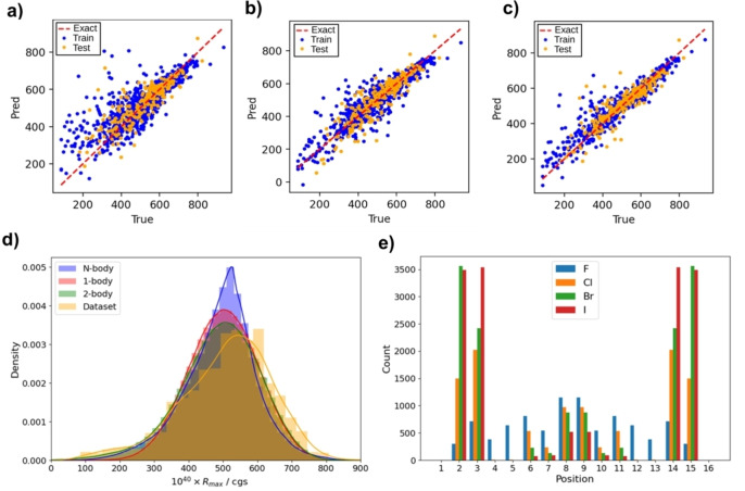
At this point, we tested a more complex case, the prediction of the highest positive R_max values for the hexahalogenated [6]helicene family, increasing the number from 200,000 to almost 19 million molecules. Here, the critical point is how to train the new model at the same level as for the Case 1. We used up to 1182 randomly selected molecules generated using the Python random library (see Supporting Information for details), and containing one to six halogens as training examples. ^[58] We observed that with the new model the predicted R_max values for halogenated[6]helicenes (Figure 6c) were slightly smaller than in Case 1 owing to training values for hexahalogenated [6]helicenes are, in general, smaller. Such full data set presents a R_mean value of 508 (Figure 6d) with very few cases with R_max beyond 800.

Figure 6.

Correlation between model‐predicted (y axis) vs DFT‐calculated (x axis) rotational strength (R, 10⁻⁴⁰ cgs units) values for halo[6]helicenes up to 6 halogen atoms (N=1182 [6]helicenes) employing a) 1‐body, b) 2‐body, c) N‐body models. The statistical parameters of the models can be found in Table S17. d) Distributions of positive R_max obtained from DFT, 1‐, 2‐, and N‐body models for hexahalogenated[6]helicenes. e) Location of halogens in molecules with high obtained from N‐body model for hexahalogenated[6]helicenes.

Then, 1‐ and 2‐body (Figure 6a‐b) models were created, both presenting a reasonable correlation. This suggests that a kind of parameterization is again present in the physics of the system, presenting α_i and β_i coefficients for both cases common main features (SI, Tables S2–S11 for Case 1 and Tables S18–S27 for Case 2). Among them, it is worth highlighting that the higher the substitution, the lower the R_max value. Furthermore, the 2‐body model presented a better correlation than in Case 1, which is reasonable since the database now includes more examples of adjacently substituted helicenes.

With the three models in hand, the R_max value distributions for the total 1.64×10⁷ hexahalogenated[6]helicenes were predicted, providing quite similar distributions. The N‐body one is slightly narrower and properly fits the DFT R_max value distribution (Figure 6d). Again, the substitution increase seems to be detrimental for high R_max values, which is in qualitative agreement with the underlying physics from case 1. Additional substituents disfavour the electronic circulation of the π conjugated system during the transition, minimizing |m_0j | values. If that assumption is correct, higher substitution numbers from hepta‐ to hexadecahalogenated [6]helicenes would always yield poorer chiroptical responses. The model suggested good hexahalogenated [6]helicene candidates (ca. 20) with high values of R_max (>910) (Table S28). All have bromine/iodine atoms in positions 2,3(14,15), supporting the conclusions from Case 1, and the smallest fluorine/chlorine atoms in the furthest 8–9 positions (Figure 6e and 7). All were evaluated by DFT (Table S28), but neither resulted in R_max values higher than the obtained one for privileged compound 1.

Figure 7.

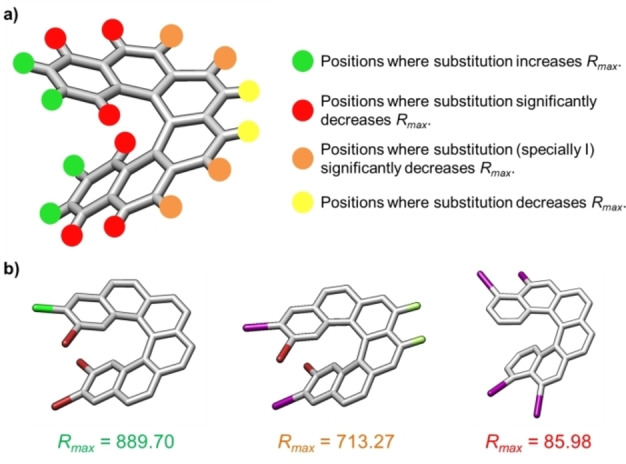
a) Role of position and nature of the substitution in [6]helicenes and b) Examples of derivatives with high, normal and low R _max values. Color code: iodine, violet; bromine, brown; chlorine, green; fluorine, pale green.

Case 3. Positive R_max values from hepta‐ to hexadecahalogenated (P)‐[6]helicenes

To check if the models developed in Case 2 remains valid for hepta‐ to hexadecahalogenated [6]helicenes, we computed 1000 randomly selected examples (100 samples each family) and we compared the DFT values with the predictions of the models. Figure 8a shows the DFT‐calculated R_max values and those predicted by the N‐body model for the 100 heptahalogen[6]helicenes. Regarding DFT examples, the decrease of R_max value is clearly consistent with the conclusions of cases 1 and 2 (Figures S10–S19). 1‐Body model, despite its simplicity, gives again a reasonable agreement, catching the main feature of maximizing |m_0j | value, which is essentially dependent of the halogen position. In general, the 2‐body model becomes invalid (e.g. Figure S19) with higher halogenation levels and even provides negative R_max . This observation can be reasoned as follows: the primary conclusion of the 2‐body model is that two adjacent halogens lead to a decrease in R_max , as quantified by the β_i coefficients. When a model based on this premise is applied to helicenes with more neighboring halogens (resulting from increased substitution), it is consistent to observe much lower R_max values. The 1‐body model, which considers only the position of the halogens, continues to provide accurate predictions. Finally, N‐Body model, although less interpretable, deals with such multiple interactions owing to the nature of the model. It remains valid, reporting suitable values for higher halogenations degrees even being trained using only up to six halogens.

Figure 8.

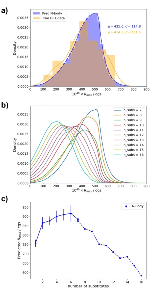
a) Distributions of positive R_max obtained from DFT and N‐body model for heptahalogenated [6]helicenes, including mean (μ) and standard deviation (σ). Predicted R _max distributions (b) and evolution of the largest R _max values (c) using N‐body model for [6]helicenes ranging from hepta‐ to hexadeca‐ halosubstituted ones. Predictions employing all possible molecules (solid line) and 10⁶ selected candidates of each family (dashed line). Error bars correspond to the standard deviation.

If the mentioned distributions are considered representative and a Gaussian‐type curve is assumed, an estimation of the expected values beyond some critical number can be done (Tables S29–S31). For example, the probability of finding a heptahalogenated[6]helicene with a R_max higher than 1000 is 0.000379 %, which means that despite being such small value, approximately 300 helicenes are statistically predicted. We then evaluated R_max values for the entire family of heptahalogenated [6]helicenes (9.4×10⁷ molecules). The maximum value obtained using the N‐body model was 846, in line with previous findings. The relevant thing here is that the N‐body and 1‐body predictions seem to remain essentially valid for any kind of substitution.

For higher substitutions, the values in the initial 100 examples evaluated by the 1‐body and N‐body models and DFT‐calculated values show satisfactory fitting. Therefore, a total of 10⁶ examples of each family were evaluated using the models to have a better description of the phenomena. As the number of halogens increases, the R_mean value diminishes (Figure 8b), hampering the existence of compounds with exceptional R_max values (Figure 8c). Based on the previous reasoning, the expectation for R_max values beyond 1000 10⁻⁴⁰ cgs units is spurious and no candidates with an R_max above 1150 10⁻⁴⁰ cgs units are statistically expected for any kind of substitution (Table S32). Basically, almost no halogen substitution beyond four halogen atoms in privileged positions allows a reinforcement of the optimal rotatory strength of the system.

Case 4. Negative R_max values from mono‐ to hexadecahalogenated (P)‐[6]helicenes

Negative R_max values were also evaluated using a similar approach to case 3, obtaining a reasonably good correlation within the N‐body model (Figure S21). The R_mean is smaller than in the case of positive ones and very few examples with R_max values beyond ‐850 were predicted (Table S34). Its DFT evaluation also supported the lower values. Once again some positions are preferred (3,14‐ and 5,12−), resulting from an elongation of the helicene electron density to the substituents and consequently the increase of the involved momenta associated to an electronic circulation along the C₂ axis of the [6]helicene core (Table S35 and Figure S22). Again, the 10⁶‐element simulation for each substitution degree show the R_max values strongly diminish with the substitution and no values around ‐900 can be stadistically obtained (Figure S23). This case concludes that positive R_max values are higher than negative ones in absolute value for the P‐enantiomer.

Synthesis of selected examples with exceptional chiroptical properties.

Although machine learning approaches are considered valuable for exploring the extrema of desired properties, the subsequent validation of the predictions is highly infrequent. In our case, the verification was carried out and the most outstanding candidate 1 was synthesized (See SI). In addition, 2,15‐bromo[6]helicene (2) also proposed as candidate by the models, was prepared for comparison. ^[59] Structural assignment was carried out by usual NMR techniques and by single crystal X‐ray diffraction of suitable crystals for compound 1. ^[60] The results obtained from the refinement of the diffraction data confirmed the proposed structure of the compound, revealing geometrical features similar to those of unsubstituted [6]helicene (see Supporting Information for details). ^[61]

We then studied the chiroptical properties, particularly the ECD, which has not been reported for compound 2. Experimental ones for compounds 1 and 2 are in excellent agreement with the expected ones (Figure 9). Molar circular dichroism for tetrabromo[6]helicene 1 (317 m^–1cm^–1) is higher than for the dibromo derivative (287 m^–1cm^–1), matching as well their relative intensities. These values are higher than the reported for parent [6]helicene (259 m^–1cm^–1). ^[6]

Figure 9.

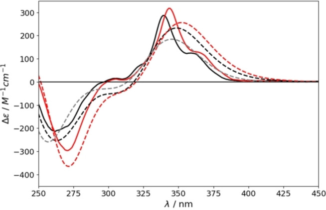
Theoretical (dashed lines) and experimental (solid lines) ECD spectra of parent [6]helicene (grey) and di‐ (black) (2) and tetrabromo (red) (1) substituted ones.

Overall, this final experimental work, validates the accuracy of the predicting models, according to their corresponding trainings. Thus, the reliability of the developed deep learning, turns it into a perfect tool on the rapid elucidation of optimal synthetic targets in order to maximize chiroptical properties.

Conclusion

Taking advantage of deep learning techniques, in this work we have developed a neutral network to predict the R_max values of billions of halogenated [6]helicenes, from one to the full hexadecahalogenated derivatives, with minimal computation cost. We have built three different models with increasing complexity (1‐body, 2‐body and N‐body respectively), whose predictions reasonably correspond with the DFT‐calculated values. Although the best correlation is always obtained with the N‐body model it is worth noting that a parameterization of R_max acquire evident physical meaning when simpler 1‐ and 2‐body models are used in derivatives with up to six halogen atoms. It has also been observed that increasing the number of halogens above four promotes a diminishing of R_max . More interestingly, we have found a structure‐properties relationship, as there are favoured positions and halogen atoms that increase its value, mainly bromine and iodine in 2,3 and 14,15 positions. An exhaustive analysis of data has been done, considering both positive and negative values of rotational strength, presenting these last lower values. Finally, the predictions have been experimentally supported by the synthesis of the two best candidates predicted by the network, confirming the optimal ECD values in excellent agreement with the predicted by the deep learning approach.

Supporting Information

The authors have cited additional references within the Supporting Information.[ ⁶² , ⁶³ , ⁶⁴ , ⁶⁵ , ⁶⁶ , ⁶⁷ , ⁶⁸ , ⁶⁹ , ⁷⁰ , ⁷¹ , ⁷² , ⁷³ , ⁷⁴ , ⁷⁵ ]

Conflict of Interests

The authors declare no conflict of interest.

Uceda R. G., Gijón A., Míguez-Lago S., Cruz C. M., Blanco V., Fernández-Álvarez F., Álvarez de Cienfuegos L., Molina-Solana M., Gómez-Romero J., Miguel D., Mota A. J., Cuerva J. M., Angew. Chem. Int. Ed. 2024, 63, e202409998. 10.1002/anie.202409998

Data Availability Statement

The data that support the findings of this study are available in the supplementary material of this article.

References

- 1. Shen Y., Chen C.-F., Chem. Rev. 2012, 112, 1463–1535. [DOI] [PubMed] [Google Scholar]
- 2. Gingras M., Chem. Soc. Rev. 2013, 42, 968–1006. [DOI] [PubMed] [Google Scholar]
- 3. Gingras M., Félix G., Peresutti R., Chem. Soc. Rev. 2013, 42, 1007–1050. [DOI] [PubMed] [Google Scholar]
- 4. Abbate S., Longhi G., Mori T., Helicenes, Wiley, 2022, pp. 373–394. [Google Scholar]
- 5. Müller T. J. J., Bunz U. H. F., Functional Organic Materials, Wiley, 2006. [Google Scholar]
- 6. Nakai Y., Mori T., Inoue Y., J. Phys. Chem. A 2012, 116, 7372–7385. [DOI] [PubMed] [Google Scholar]
- 7. Johannessen C., Blanch E. W., Villani C., Abbate S., Longhi G., Agarwal N. R., Tommasini M., Lightner D. A., J. Phys. Chem. B 2013, 117, 2221–2230. [DOI] [PubMed] [Google Scholar]
- 8. Kubo H., Hirose T., Nakashima T., Kawai T., Hasegawa J., Matsuda K., J. Phys. Chem. Lett. 2021, 12, 686–695. [DOI] [PubMed] [Google Scholar]
- 9. Mahato B., Panda A. N., J. Phys. Chem. A 2023, 127, 2284–2294. [DOI] [PubMed] [Google Scholar]
- 10. Furche F., Ahlrichs R., Wachsmann C., Weber E., Sobanski A., Vögtle F., Grimme S., J. Am. Chem. Soc. 2000, 122, 1717–1724. [Google Scholar]
- 11. Warnke I., Furche F., Wiley Interdiscip. Rev.: Comput. Mol. Sci. 2012, 2, 150–166. [Google Scholar]
- 12. LeCun Y., Bengio Y., Hinton G., Nature 2015, 521, 436–444. [DOI] [PubMed] [Google Scholar]
- 13. Margraf J. T., Angew. Chem. Int. Ed. 2023, 62, e202219170. [DOI] [PubMed] [Google Scholar]
- 14. Karthikeyan A., Priyakumar U. D., J. Chem. Sci. 2022, 134, 2. [DOI] [PMC free article] [PubMed] [Google Scholar]
- 15. Mater A. C., Coote M. L., J. Chem. Inf. Model 2019, 59, 2545–2559. [DOI] [PubMed] [Google Scholar]
- 16. Hou X., Li S., Frey J., Hong X., Ackermann L., Chem 2024, 10, 2283–2284. [Google Scholar]
- 17. Fooshee D., Mood A., Gutman E., Tavakoli M., Urban G., Liu F., Huynh N., Van Vranken D., Baldi P., Mol. Syst. Des. Eng. 2018, 3, 442–452. [Google Scholar]
- 18. Beker W., Roszak R., Wołos A., Angello N. H., Rathore V., Burke M. D., Grzybowski B. A., J. Am. Chem. Soc. 2022, 144, 4819–4827. [DOI] [PMC free article] [PubMed] [Google Scholar]
- 19. Pereira A., Trofymchuk O. S., J. Phys. Chem. C 2023, 127, 12983–12994. [Google Scholar]
- 20. Fitzner M., Wuitschik G., Koller R., Adam J.-M., Schindler T., ACS Omega 2023, 8, 3017–3025. [DOI] [PMC free article] [PubMed] [Google Scholar]
- 21. Singh S., Sunoj R. B., Acc. Chem. Res. 2023, 56, 402–412. [DOI] [PubMed] [Google Scholar]
- 22. Zhang S., Xu L., Li S., Oliveira J. C. A., Li X., Ackermann L., Hong X., Chem. Eur. J. 2023, 29, e202202834. [DOI] [PMC free article] [PubMed] [Google Scholar]
- 23. Tu Z., Stuyver T., Coley C. W., Chem Sci 2023, 14, 226–244. [DOI] [PMC free article] [PubMed] [Google Scholar]
- 24. Burés J., Larrosa I., Nature 2023, 613, 689–695. [DOI] [PubMed] [Google Scholar]
- 25. Hansen K., Biegler F., Ramakrishnan R., Pronobis W., von Lilienfeld O. A., Müller K.-R., Tkatchenko A., J. Phys. Chem. Lett. 2015, 6, 2326–2331. [DOI] [PMC free article] [PubMed] [Google Scholar]
- 26. Pinheiro G. A., Mucelini J., Soares M. D., Prati R. C., Da Silva J. L. F., Quiles M. G., J. Phys. Chem. A 2020, 124, 9854–9866. [DOI] [PubMed] [Google Scholar]
- 27. Collins E. M., Raghavachari K., J. Phys. Chem. A 2021, 125, 6872–6880. [DOI] [PubMed] [Google Scholar]
- 28. Bhat V., Sornberger P., Pokuri B. S. S., Duke R., Ganapathysubramanian B., Risko C., Chem. Sci. 2023, 14, 203–213. [DOI] [PMC free article] [PubMed] [Google Scholar]
- 29. Nguyen T. H., Le K. M., Nguyen L. H., Truong T. N., ACS Omega 2023, 8, 38441–38451. [DOI] [PMC free article] [PubMed] [Google Scholar]
- 30. Weiss T., Wahab A., Bronstein A. M., Gershoni-Poranne R., J. Org. Chem. 2023, 88, 9645–9656. [DOI] [PubMed] [Google Scholar]
- 31. Karuth A., Casanola-Martin G. M., Lystrom L., Sun W., Kilin D., Kilina S., Rasulev B., J. Phys. Chem. Lett. 2024, 15, 471–480. [DOI] [PubMed] [Google Scholar]
- 32. Sigmund L. M., Sowndarya S., Albers A., Erdmann P., Paton R. S., Greb L., Angew. Chem. Int. Ed. 2024, 63, e202401084. [DOI] [PubMed] [Google Scholar]
- 33. Orsi M., Shing Loh B., Weng C., Ang W. H., Frei A., Angew. Chem. Int. Ed. 2024, 63, e202317901. [DOI] [PubMed] [Google Scholar]
- 34. Dral P. O., Chem. Commun. 2024, 60, 3240–3258. [DOI] [PubMed] [Google Scholar]
- 35. Keith J. A., Vassilev-Galindo V., Cheng B., Chmiela S., Gastegger M., Müller K.-R., Tkatchenko A., Chem. Rev. 2021, 121, 9816–9872. [DOI] [PMC free article] [PubMed] [Google Scholar]
- 36. Aldossary A., Campos-Gonzalez-Angulo J. A., Pablo-García S., Xuan-Leong S., Rajaonson E. M., Thiede L., Tom G., Wang A., Avagliano D., Aspuru-Guzik A., Adv. Mater. 2024, 36, 2402369. [DOI] [PubMed] [Google Scholar]
- 37. Ju C.-W., Shen Y., French E. J., Yi J., Bi H., Tian A., Lin Z., J. Phys. Chem. A 2024, 128, 2457–2471. [DOI] [PubMed] [Google Scholar]
- 38. Faber F. A., Hutchison L., Huang B., Gilmer J., Schoenholz S. S., Dahl G. E., Vinyals O., Kearnes S., Riley P. F., von Lilienfeld O. A., J. Chem. Theory Comput. 2017, 13, 5255–5264. [DOI] [PubMed] [Google Scholar]
- 39. Huang B., von Rudorff G. F., von Lilienfeld O. A., Science 2023, 381, 170–175. [DOI] [PubMed] [Google Scholar]
- 40. Smith J. S., Isayev O., Roitberg A. E., Chem. Sci. 2017, 8, 3192–3203. [DOI] [PMC free article] [PubMed] [Google Scholar]
- 41. Zhang H., Juraskova V., Duarte F., Nat. Commun. 2024, 15, 6114. [DOI] [PMC free article] [PubMed] [Google Scholar]
- 42. Kuznetsova V., Coogan Á., Botov D., Gromova Y., Ushakova E. V., Gun'ko Y. K., Adv. Mater. 2024, 36, 2308912. [DOI] [PMC free article] [PubMed] [Google Scholar]
- 43. Schrier J., Norquist A. J., Buonassisi T., Brgoch J., J. Am. Chem. Soc. 2023, 145, 21699–21716. [DOI] [PubMed] [Google Scholar]
- 44. Rodríguez R., Naranjo C., Kumar A., Matozzo P., Das T. K., Zhu Q., Vanthuyne N., Gómez R., Naaman R., Sánchez L., Crassous J., J. Am. Chem. Soc. 2022, 144, 7709–7719. [DOI] [PMC free article] [PubMed] [Google Scholar]
- 45. Dhbaibi K., Abella L., Meunier-Della-Gatta S., Roisnel T., Vanthuyne N., Jamoussi B., Pieters G., Racine B., Quesnel E., Autschbach J., Crassous J., Favereau L., Chem. Sci. 2021, 12, 5522–5533. [DOI] [PMC free article] [PubMed] [Google Scholar]
- 46. Kettner M., Maslyuk V. V., Nürenberg D., Seibel J., Gutierrez R., Cuniberti G., Ernst K.-H., Zacharias H., J. Phys. Chem. Lett. 2018, 9, 2025–2030. [DOI] [PubMed] [Google Scholar]
- 47. Kiran V., Mathew S. P., Cohen S. R., Hernández Delgado I., Lacour J., Naaman R., Adv. Mater. 2016, 28, 1957–1962. [DOI] [PubMed] [Google Scholar]
- 48. Hammett L. P., J. Am. Chem. Soc. 1937, 59, 96–103. [Google Scholar]
- 49. Lee A., Sarker S., Saal J. E., Ward L., Borg C., Mehta A., Wolverton C., Commun. Mater. 2022, 3, 73. [Google Scholar]
- 50. Taniike T., Takahashi K., Nat. Catal. 2023, 6, 108–111. [Google Scholar]
- 51. Strieth-Kalthoff F., Sandfort F., Kühnemund M., Schäfer F. R., Kuchen H., Glorius F., Angew. Chem. Int. Ed. 2022, 61, e202204647. [DOI] [PubMed] [Google Scholar]
- 52.M. J. Frisch, G. W. Trucks, H. B. Schlegel, G. E. Scuseria, M. A. Robb, J. R. Cheeseman, G. Scalmani, V. Barone, B. Mennucci, G. A. Petersson, H. Nakatsuji, M. Caricato, X. Li, H. P. Hratchian, A. F. Izmaylov, J. Bloino, G. Zheng, J. L. Sonnenberg, M. Hada, M. Ehara, K. Toyota, R. Fukuda, J. Hasegawa, M. Ishida, T. Nakajima, Y. Honda, O. Kitao, H. Nakai, T. Vreven, J. A. Montgomery Jr., J. E. Peralta, F. Ogliaro, M. Bearpark, J. J. Heyd, E. Brothers, K. N. Kudin, V. N. Staroverov, R. Kobayashi, J. Normand, K. Raghavachari, A. Rendell, J. C. Burant, S. S. Iyengar, J. Tomasi, M. Cossi, N. Rega, J. M. Millam, M. Klene, J. E. Knox, J. B. Cross, V. Bakken, C. Adamo, J. Jaramillo, R. Gomperts, R. E. Stratmann, O. Yazyev, A. J. Austin, R. Cammi, C. Pomelli, J. W. Ochterski, R. L. Martin, K. Morokuma, V. G. Zakrzewski, G. A. Voth, P. Salvador, J. J. Dannenberg, S. Dapprich, A. D. Daniels, O. Farkas, J. B. Foresman, J. V. Ortiz, J. Cioslowski, D. J. Fox, Gaussian09. Revission B.01., 2010.
- 53. Abadi M., Agarwal A., Barham P., Brevdo E., Chen Z., Citro C., Corrado G. S., Davis A., Dean J., Devin M., Ghemawat S., Goodfellow I., Harp A., Irving G., Isard M., Jia Y., Jozefowicz R., Kaiser L., Kudlur M., Levenberg J., Mané D., Monga R., Moore S., Murray D., Olah C., Schuster M., Shlens J., Steiner B., Sutskever I., Talwar K., Tucker P., Vanhoucke V., Vasudevan V., Viégas F., Vinyals O., Warden P., Wattenberg M., Wicke M., Yu Y., Zheng X., arXiv 2016, 1603.04467. [Google Scholar]
- 54.Among these metrics, MAE represents the mean of the absolute differences between the predicted and the actual values, assigning equal weight to all error values, thereby mitigating the impact of outliers. By contrast, MSE calculates the mean of the squared differences between the predicted and the actual values, amplifying the influence of larger errors, thus more susceptible to outliers.
- 55. Uceda R. G., Cruz C. M., Míguez-Lago S., de Cienfuegos L. Á., Longhi G., Pelta D. A., Novoa P., Mota A. J., Cuerva J. M., Miguel D., Angew. Chem. Int. Ed. 2024, 63, e202316696. [DOI] [PubMed] [Google Scholar]
- 56. Lu T., Chen F., J. Comput. Chem. 2012, 33, 580–592. [DOI] [PubMed] [Google Scholar]
- 57. Nakai Y., Mori T., Inoue Y., J. Phys. Chem. A 2013, 117, 83–93. [DOI] [PubMed] [Google Scholar]
- 58.Such number was the result of a steady increase of examples until the N-body correlation remained statistically stable with a MAE of 27 10–40 cgs units for train and 36 10–40 cgs for test (see Figure S3).
- 59. Schulte T. R., Holstein J. J., Clever G. H., Angew. Chem. Int. Ed. 2019, 58, 5562–5566. [DOI] [PMC free article] [PubMed] [Google Scholar]
- 60.Deposition Number CCDC 2341175 Contains the Supplementary Crystallographic Data for This Paper. These Data Are Provided Free of Charge by the Joint Cambridge Crystallographic Data Centre and Fachinformationszentrum Karlsruhe Access Structures Service www.ccdc.cam.ac.uk/structures.
- 61. Dračínský M., Storch J., Církva V., Císařová I., Sýkora J., Phys. Chem. Chem. Phys. 2017, 19, 2900–2907. [DOI] [PubMed] [Google Scholar]
- 62. Abbate S., Lebon F., Longhi G., Fontana F., Caronna T., Lightner D. A., Phys. Chem. Chem. Phys. 2009, 11, 9039. [DOI] [PubMed] [Google Scholar]
- 63. Hellou N., Macé A., Martin C., Dorcet V., Roisnel T., Jean M., Vanthuyne N., Berrée F., Carboni B., Crassous J., J. Org. Chem. 2018, 83, 484–490. [DOI] [PubMed] [Google Scholar]
- 64. Becke A. D., J. Chem. Phys. 1993, 98, 5648–5652. [Google Scholar]
- 65. Zhao Y., Truhlar D. G., Theor. Chem. Acc. 2008, 120, 215–241. [Google Scholar]
- 66. Vydrov O. A., Scuseria G. E., J. Chem. Phys. 2006, 125, 234109. [DOI] [PubMed] [Google Scholar]
- 67. Krishnan R., Binkley J. S., Seeger R., Pople J. A., J. Chem. Phys. 1980, 72, 650–654. [Google Scholar]
- 68. Schäfer A., Horn H., Ahlrichs R., J. Chem. Phys. 1992, 97, 2571–2577. [Google Scholar]
- 69. Bergner A., Dolg M., Küchle W., Stoll H., Preuß H., Mol. Phys. 1993, 80, 1431–1441. [Google Scholar]
- 70. Hehre W. J., Ditchfield R., Pople J. A., J. Chem. Phys. 1972, 56, 2257–2261. [Google Scholar]
- 71. Miertuš S., Scrocco E., Tomasi J., Chem. Phys. 1981, 55, 117–129. [Google Scholar]
- 72. Andrus M. B., Harper K. C., Christiansen M. A., Binkley M. A., Tetrahedron Lett. 2009, 50, 4541–4544. [Google Scholar]
- 73. Sheldrick G. M., Acta Crystallogr. A Found Adv. 2015, 71, 3–8. [DOI] [PMC free article] [PubMed] [Google Scholar]
- 74. Sheldrick G. M., Acta Crystallogr. A 2008, 64, 112–122. [DOI] [PubMed] [Google Scholar]
- 75. Farrugia L. J., J. Appl. Crystallogr. 2012, 45, 849–854. [Google Scholar]
Associated Data
This section collects any data citations, data availability statements, or supplementary materials included in this article.