

Abstract
One of the most intense geomagnetic storms of recent times occurred on 10–11 May 2024. With a peak negative excursion of Sym‐H below −500 nT, this storm is the second largest of the space era. Solar wind energy transferred through radiation and mass coupling affected the entire Geospace. Our study revealed that the dayside magnetopause was compressed below the geostationary orbit (6.6 RE) for continuously ∼6 hr due to strong Solar Wind Dynamic Pressure (SWDP). Tremendous compression pushed the bow‐shock also to below the geostationary orbit for a few minutes. Magnetohydrodynamic models suggest that the magnetopause location could be as low as 3.3RE. We show that a unique combination of high SWDP (≥15 nPa) with an intense eastward interplanetary electric field (IEFY ≥ 2.5 mV/m) within a super‐dense Interplanetary Coronal Mass Ejection lasted for 409 min–is the key factor that led to the strong ring current at much closer to the Earth causing such an intense storm. Severe electrodynamic disturbances led to a strong positive ionospheric storm with more than 100% increase in dayside ionospheric Total Electron Content (TEC), affecting GPS positioning/navigation. Further, an HF radio blackout was found to occur in the 2–12 MHz frequency band due to strong D‐ and E‐region ionization resulting from a solar flare prior to this storm.
Keywords: solar wind, interplanetary coronal mass ejection, ring current, geomagnetic storm
Key Points
Strong SWDP caused a highly compressed magnetosphere with magnetopause pushed below geostationary orbit (6.6 RE) continuously for 6 hr
The highly compressed magnetosphere led an intense ring current at much closer distance to the Earth
A super‐dense ICME with high SWDP (>15 nPa) and IEFY (>2.5 mV/m) sustaining for 409 min ‐ a key factor responsible for this intense storm
1. Introduction
The Earth's magnetosphere is constantly exposed to a continuum of charged particles emitted from the Solar corona, known as Solar Wind. The transfer of solar wind energy and momentum to the Earth's environment triggers large‐scale plasma flows (and currents) in the magnetosphere and ionosphere. These magnetospheric and ionospheric currents produce additional magnetic fields that are additive/suppressive to the Earth's main field, thereby contributing to the short‐term, but highly dynamic changes in the geomagnetic field. Solar storms often release enormous bursts of electromagnetic energy (solar flares) followed by massive ejections of coronal mass (CMEs). The elevated doses of solar wind particles during CMEs exert additional pressure on the Earth's magnetosphere and cause significant compression of the magnetopause (Sibeck et al., 1991). Furthermore, enhanced solar wind particle injection into the magnetosphere drives a strong toroidal current around Earth, known as ring current, at distances of 4–7 Earth radii (RE) (Akasofu et al., 1963; Daglis et al., 1999). The additional magnetic field produced by this ring current is directed southward (opposite to Earth's magnetic field), thereby causing a depression in the net magnetic field measured on the ground. The magnitude of the geomagnetic field decrease on the ground varies with the measurement location and local time. The longitudinally averaged disturbance in the geomagnetic H‐component field at low to mid‐latitudes, represented by Dst and Sym‐H indices (Imajo et al., 2022; Iyemori et al., 1992; Sugiura, 1991), are generally used to quantify the intensity of the storms. A significant decrease of Sym‐H, say below −50 nT, qualifies to be called a geomagnetic storm. At the same time, several categories with nomenclature such as weak (−100 to −50 nT), moderate (−200 to −100 nT), intense (−400 to −200 nT), and super‐intense (−400 nT or less) storms can be found in the literature (although no strict definitions exist). The intensity of the ring current and its proximity to the Earth determine the magnitude of disturbance observed in the surface magnetic field (Daglis et al., 1999; Vallat et al., 2005). At the same time, the intensity and location of the ring current, in turn, depend on the incoming solar wind forcing and its magnetospheric coupling efficiency (Daglis et al., 1999).
The recent geomagnetic storm on 10–11 May 2024 engendered a great interest among enthusiastic civilians and aurora watchers across the globe. Early reports show aurora sightings by the naked eye and/or by simple smartphone cameras (besides the conventional scientific instruments) extending down to latitudes as low as ∼30° (Grandin et al., 2024; Hayakawa et al., 2024). This storm drew great attention from the scientific community by its magnitude surpassing the −500 nT mark in the Sym‐H indexThe Sym‐H surpassing the −500 nT also makes it the largest storm in the past three decades and the second largest in the history of the space age (after the 13 March 1989 storm).
In this study, we investigate the factors and possible mechanisms that led to this super‐intense storm in comparison with other intense storms that occurred in the past, and the key findings are reported here. Additionally, we detail the drastic reconfiguration of the magnetosphere‐ionosphere system and the resultant effects on the geomagnetic field and ionospheric electron content during this storm and a solar flare that occurred prior to this storm.
2. Data
A wide set of space‐borne and ground‐based measurements alongside magnetohydrodynamic (MHD) simulations are employed in this study. The X‐ray flux measurements at short (0.5–4.0 Å) and long (1.0–8.0 Å) wavelengths from Extreme Ultraviolet and X‐ray Irradiance Sensors (EXIS) on board the Geostationary Operational Environmental Satellites (GOES) (Machol et al., 2020) are examined to detect the solar flare occurrences. The solar wind particle and magnetic field measurements from the Deep Space Climate Observatory (DSCOVR) near the first Lagrange (L1) point were used to investigate the solar wind conditions that led to this intense storm. The calibrated Level‐2 data from Faraday Cup and Magnetometer payloads available at 1‐min resolution are considered (Loto'aniu et al., 2022) in this study. A network of ground‐based flux gate magnetometers spread across the Indian equatorial and low‐latitudes (IIG, 2024) have been used to investigate the geomagnetic field disturbances that occurred during this storm. The VLF signal amplitude recorded by an NWC receiver (Lohrey & Kaiser, 1979; Xia et al., 2020) and ionograms from a Canadian Advanced Digital Ionosonde (CADI) (MacDougall et al., 1995) are used to examine the disturbances in the ionospheric D‐ and F‐regions during a solar flare that occurred prior to this storm. The list of stations hosting the magnetometers, VLF receiver, and Ionosonde over the Indian region, along with their locations, are provided in Supporting Information S1.
Further, the BATSRUS (Block‐Adaptive‐Tree‐Solarwind‐Roe‐Upwind‐Scheme) global magnetospheric MHD model (Harel et al., 1981; Powell et al., 1999) coupled with Rice Convection Model (RCM) (Toffoletto et al., 2003) and Ridley Ionospheric Model (RIM) (Ridley et al., 2004) is used to examine the location of magnetopause (LMP) and to investigate the ring current intensity. The BATSRUS had been run under the Space Weather ‘Modeling Framework (SWMF) at the Community Coordinate Modeling Center (CCMC) platform for the given solar wind inputs obtained from DSCOVR.
3. Results and Discussion
3.1. Sources of the Storm
During 8–10 May 2024, a series of solar flares and CMEs erupted from the sunspot group AR36648. Figure 1 shows the X‐ray flux at short (0.5–4 Å, red curve) and long (1.0–8.0 Å, blue curve) wavelengths monitored by the GOES during this period. Several solar flares that occurred during this period are evident as sharp enhancements in the X‐ray flux. Six X‐class flares occurred during this period as shown in Figure 1. The peak X‐ray flux timings of these flares were 0141, 0509, 2140 UT on 8 May 2024, 0913 UT, 1744 UT on 9 May 2024, and 0654 UT on 10 May 2024. CMEs followed all these six X‐class flares after a few minutes (Hayakawa et al., 2024). The fast and dense solar wind structures from these CMEs interacted with one another, forming a composite Interplanetary CME (ICME) with complex solar wind density and magnetic field structures embedded. Figure 2 depicts the complex variations of solar wind velocity (V), density (N), temperature (T), and total scalar interplanetary magnetic field (B T) associated with this ICME measured by NASA's Deep Space Climate Observatory (DSCOVR) satellite at the first Lagrangian (L1) point. The sudden and large excursions in all the solar wind parameters (V, N, T, and B T) at 1634 UT on 10 May 2024, mark the arrival of ICME forward shock. Another distinct and simultaneous increase in all the solar wind parameters can be observed at 2136 UT, indicating the possible arrival of a second ICME. Assuming average speeds around ∼950–1,100 km/s, one can roughly relate the CMEs associated with (or after) the flares that occurred at 2140 UT on 8 May 2024 and 0913 UT on 9 May 2024 are likely the sources of the two ICME observed at 1,634 and 2136 UT at L1‐point by DSCOVR, respectively. Subsequently, sharp increases in the geomagnetic field were observed globally in ground‐based magnetometers at 1705 UT and 2221 UT (not shown in the figure). This indicates the travel times of the first and second ICMEs from L1‐point to Earth's magnetosphere as 31 and 45 min, respectively.
Figure 1.
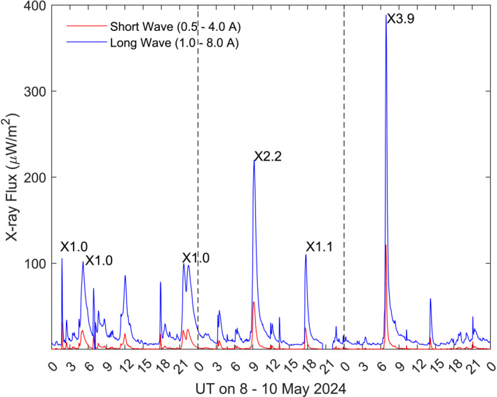
X‐ray flux measured from GOES satellite at geostationary orbit showing the occurrence of a series of solar flares during 8–10 May 2024. Six X‐class flares are indicated in the Figure.
Figure 2.
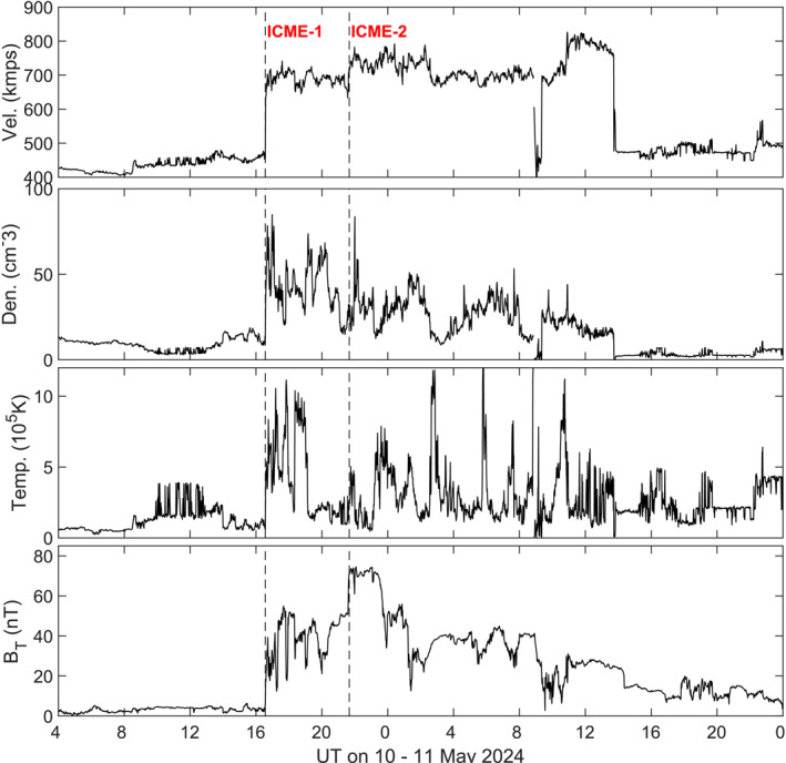
UT variations of solar wind velocity (V), density (N), temperature (T), and total scalar interplanetary magnetic field (IMF B T). The arrival of ICME shock at 1634 UT, and a likely second shock at 2136 UT are marked as vertical dashed lines.
Figure 3a shows the variation of vertical (IMF Bz, black curve) and dawn‐to‐dusk (IMF By, red curve) components of the interplanetary magnetic field and Figure 3b shows the variation of geomagnetic storm index, Sym‐H (Imajo et al., 2022). Note that IMF data is time‐shifted by 31 min to account for the travel time of ICME from L1‐point to Earth's bow‐shock The storm sudden commencement (SSC) can be observed at 1705 UT with the arrival of first ICME shock. The Sym‐H initially exhibited a brief enhancement (for ∼10 min) and reached 88 nT due to increased magnetopause current (Araki, 1977). Subsequently, Sym‐H decreased to a minimum of −518 nT at 0214 UT on 11 May 2024. The total decrease (range) of Sym‐H is 606 nT. The arrival of second ICME can also be identified as a sharp enhancement in Sym‐H at 2221 UT. The red curve in Figure 3b is the Dst‐index computed at 1‐min time resolution (equivalent to Sym‐H) by the Block‐Adaptive‐Tree‐Solarwind‐Roe‐Upwind‐Scheme (BATSRUS) MHD model coupled with RCM and RIM models. It can be seen from this figure that BATSRUS Dst also rapidly decreased, indeed more rapidly than the observed Sym‐H, during the first few hours of the main phase that is, up to ∼2145 UT. Around 2221 UT, with the arrival of the second ICME, the BATSRUS Dst (and also Sym‐H) exhibited a sharp increase (recovery) due to the northward (eastward) turning of IMF Bz (By) (Figure 3a) and partly due to enhanced magnetopause currents. Both the Sym‐H and BATSRUS Dst decreased again with the southward turning of IMF Bz, and the main phase of the storm continued. However, the BATSRUS Dst is remained significantly higher than the Sym‐H throughout the rest of the storm. While the peak negative Sym‐H of −518 nT occurred at ∼0214 UT, the peak negative in BATSRUS Dst (−342 nT) occurred around 0745 UT on 11 May 2024. In brief, the BATSRUS significantly underestimated the storm intensity after the arrival of the second ICME. The observed deviations in the BATSRUS Dst with respect to Sym‐H could be due to the method of deriving the Dst in the model. In the BATSRUS model under SWMF, the Dst index is calculated by computing the ground perturbations, through Biot‐Savart law integrals, caused by the magnetospheric currents, field‐aligned currents (FAC), and the ionospheric Pedersen and Hall currents (Yu et al., 2010; Leihmohn et al., 2018). Although the detailed investigation of contributions from different current systems is beyond the scope of this paper, we speculate that the insufficient representation of magnetospheric currents (mainly the ring current) could be one of the important sources for the observed deviation in the BATSRUS Dst. The contributions from the FAC and ionospheric Pedersen and Hall currents are generally expected to be very small at low latitudes, and to the Dst (Yu et al., 2010).
Figure 3.
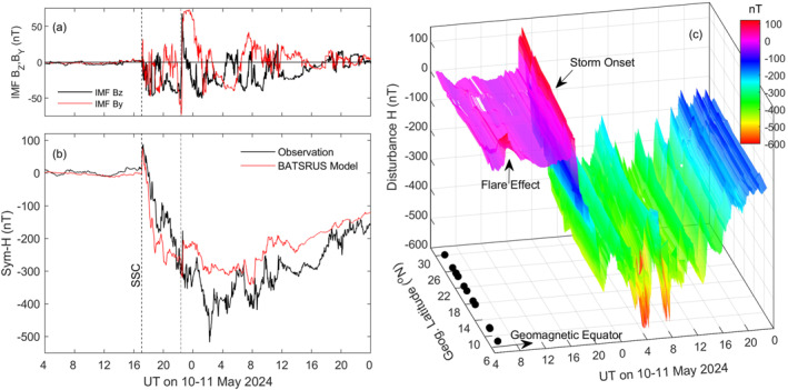
(a–b) UT variations of vertical and dawn‐dusk components of interplanetary magnetic field (IMF B z and B Y, top panel), and Sym‐H (bottom panel). (c) Latitudinal distribution of isturbance in geomagnetic H‐component field observed from the Indian network of magnetometers. The latitudes of magnetometer stations are indicated as black dots in Figure 3c.
Figure 3c shows the latitudinal distribution of disturbance in the H‐component observed from a chain of low‐latitude magnetometers from the Indian sector. The latitudes of magnetometer stations are shown as black dots, and the geomagnetic equator is indicated with an arrow in the figure. The complete list of magnetometer stations and their geographic locations are shown (Figure S1 and Table S1 in Supporting Information S1). The disturbance in the horizontal (H‐) component at different stations is computed by subtracting the H‐component variation of a previously quiet day (9 May 2024) from the variations of storm days (10 and 11 May 2024) for the respective stations. It can be noticed that the peak disturbance‐H was nearly −600 nT at latitudes close to the geomagnetic equator and exhibits slightly lower values away from the equator. A sharp positive disturbance in H due to the onset of solar flare around ∼0650 UT can also be seen in Figure 3c. This enhancement in H due to the solar flare is more prominent (∼105 nT) close to the equator, while the amplitudes were reduced sharply at latitudes northward of the equator. This equatorial enhancement in H during the solar flare is mainly due to the enhanced E‐region conductivity by X‐ray photoionization, which will be further amplified at the equator by the Cowling effect (Rastogi et al., 1999, 2017; Sripathi et al., 2013). It may also be noted that the magnetometer stations are spread over 70.74°E–92.76°E longitudes (see Figure S1 and Table S1 in Supporting Information S1), which may introduce minor local time‐dependent variations in E‐region conductivities. However, it would not much effect the results presented in Figure 3c, as it shows the disturbance H (residual) after the removal of diurnal variation, as mentioned above. Hence, the minor differences in the local times, and the resultant differences in E‐region conductivities (if any) due to longitudinal separation are ignored here.3.2 Key Factors and Possible Mechanisms.
The factors responsible for this super‐intense storm are investigated in Figure 4. The top panel shows the UT variation of solar wind dynamic pressure (SWDP), which exhibits several oscillations but has remained at high levels (>15 nPa) for several hours since the arrival of the first ICME shock. Here, where N and V are the solar wind density and velocity, respectively, and is the proton mass. Figures 4b and 4c show the Bz and By components (black curves) measured from the GOES‐18 (137oW longitude, 6.6 RE altitude). Before the arrival of ICME, the GOES‐18 was well within the Earth's magnetosphere, measuring Bz and By to be around 100 and 30 nT, respectively. Sudden changes in the Bz and By can be observed with the arrival of ICME at 1705 UT, and within a few minutes, the Bz measured by GOES‐18 turned southward. Bz and By measured by GOES‐18 exhibit rapid fluctuations (due to turbulence) in the magnetic field. The southward turning of Bz and the turbulence in Bz and By indicate that GOES‐18 was indeed measuring the shocked IMF outside the magnetopause (in the magnetosheath region). The strong SWDP exerted by ICME pushed the magnetopause below the geostationary orbit (6.6 R E), exposing the GOES‐18 to shocked and turbulent IMF in the magnetosheath region.
Figure 4.
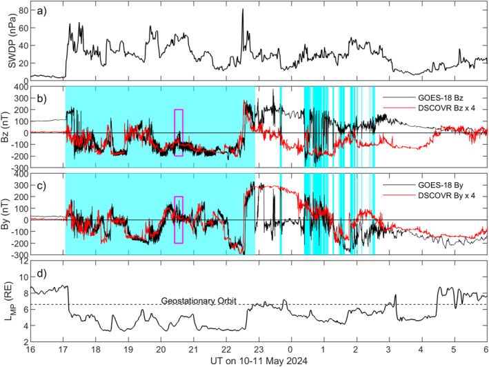
UT variations of (a) SWDP (b)–(c) Bz and By from GOES‐18 (black) and DSCOVR (red) satellites, (d) Magnetopause location (LMP) from BATSRUS model. The shaded region indicates the intervals when the magnetopause is pushed below the geostationary orbit (6.6 RE), thereby exposing GOES‐18 to shocked solar wind in the magnetosheath. The pink box in panels (b) and (c) indicates the time period expanded and shown in Figure 5, wherein the bow‐shock also pushed below the geostationary orbit for about 3 min.
The red curves in Figures 4b and 4c are the IMF Bz and By measured by DSCOVR satellite at L1. Here, the Bz and By from DSCOVR are multiplied by 4 for a better comparison with GOES‐18 observations. It is interesting to see that the Bz and By from GOES‐18 at 6.6 R E followed similar variations to those from DSCOVR at L1. These observations reveal two important facts: (a) the magnetopause was pushed to below 6.6 RE continuously for ∼6 hr (1705–2252 UT), and (b) the IMF Bz and By were amplified ∼4 times due to compression/accumulation of flux in the magnetosheath. The decrease of SWDP around 2252 UT caused relaxation of magnetopause to above 6.6 RE, as seen from the clear deviation of Bz and By measured by GOES‐18 from the DSCOVR measurements. However, variations in the SWDP caused several geostationary orbit crossings (compressions and relaxations) of magnetopause during the next 4 hours. The shaded area in light blue [Figures 4b and 4c] indicates the times when the magnetopause was pushed below the GOES‐18 orbit. Figure 4d shows the variation of magnetopause location, LMP (the minimum distance of magnetopause (boundary of closed field lines) from Earth within ±30° longitudes (i.e., 1,000 to 1,400 MLT) from the Sun‐Earth lineestimated by the BATSRUS MHD model. The model also predicted the magnetopause location below the geostationary orbit during ∼1705–∼2300 UT. which is consistent with that inferred from the GOES‐18 observations. The model results further indicate that the LMP was pushed to as low as 3.31 R E at 1852 UT and about 3.34 R E at 2222 UT. Another interesting observation of severe compression of Earth's magnetosphere and magnetosheath is presented in Figure 5. The panels from top to bottom display the variations of Bx, By and Bz components (black curves) measured by GOES‐18 at 6.6 RE, respectively. The red curves represent the IMF Bx, By and Bz from the DSCOVR at L1‐point. The GOES‐18 observations of Bx, By, and Bz exhibit rapid fluctuations, indicating turbulence in the shocked IMF in the magnetosheath region. Interestingly, one can observe that the turbulence was absent for a brief period of ∼3 min during ∼2030–2033 UT. During this period, the magnetic field components measured by GOES‐18 were nearly identical to those from DSCOVR. This suggests that the GOES‐18 was indeed going out of the bow‐shock region and measuring the unshocked IMF. In other words, the strong compression conditions led even the bow‐shock to be pushed below the geostationary orbit (6.6 RE) during this brief period. Therefore, the results from Figures 4 and 5 indicate the strongly compressive conditions of the Earth's magnetosphere and the bow‐shock prevailed during this storm period. Similar compressions of magnetopause and bow‐shock inside the geostationary orbit were earlier reported for the 31 March 2001 storm (Ober et al., 2002).
Figure 5.
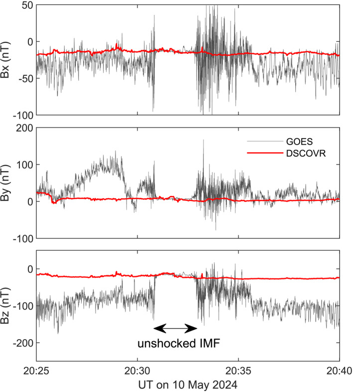
Variations of Bx, By and Bz measured from GOES‐18 at 6.6 RE (black) and the DSCOVR at L1‐point (red). The period when Earth's magnetospheric bow shock is compressed below the geostationary orbit and allowing the GOES‐18 to measure the unshocked IMF is indicated in the figure.
When the particles in the magnetosphere flow toward the Earth, they encounter an increasingly strong magnetic field. The positive gradient of the geomagnetic field is further amplified due to the compression of the magnetosphere. Consequently, the particles undergo a rapid transverse motion due to a stronger gradient drift force, and the resulting ring current flows at much closer distances to the Earth (Daglis et al., 1999 and references therein]. The more the magnetosphere is compressed, the more intense the ring current becomes and the closer it flows to the Earth. However, the location of the magnetopause is influenced by two factors: (a) the geomagnetic pressure balance with the SWDP (Holzer & Slavin, 1978) and (b) erosion of the magnetosphere via magnetic reconnection with IMF, which maximizes during the intense southward‐oriented IMF Bz (Maezawa, 1974). Southward IMF Bz also facilitates enhanced injection of solar wind particles into the magnetosphere, then to the ring current region (Dungey, 1961). A potent combination of strong SWDP and intense southward IMF Bz can push the magnetopause to much lower distances, guiding the intense ring current to flow much closer to the Earth. This was what occurred during this storm, where the SWDP was maintained above 15 nPa throughout the main phase (except for a few brief intervals), and the IMF Bz turned strongly southward for several sustained intervals.
The ICME structures that trigger geomagnetic storms typically comprise a forward shock and a high‐density sheath, followed by a low‐density and high‐magnetic field cloud region (Burlaga et al., 1998; Gopalswamy, 2006). The sheath region exerts strong SWDP on the magnetosphere; however, the highly fluctuating IMF (Temmer & Bothmer, 2022) may not facilitate a stable dayside reconnection. The major part of the geomagnetic storm's main phase develops with the arrival of a low‐density (low SWDP) magnetic cloud with sustained southward Bz (Temmer & Bothmer, 2022; Burlaga et al., 1982; Lepping et al., 1997; Gonzalez & B. Tsurutani, 1987; Gonzalez et al., 2011; Kilpua et al., 2017; Liu et al., 2020). However, in the present storm case, a series of CMEs interacted with each other and formed a composite ICME on their journey to Earth. At least two distinct ICMEs can be identified around 1634 UT and 2136 UT within this composite ICME from the solar wind observations at L1‐point. This composite ICME structure consisted of a rare and unique combination of elevated SWDP (high‐density) and sustained southward IMF Bz for several hours.
To highlight the uniqueness of this ICME structure and the resultant storm, a comparison of the most intense geomagnetic storms with peak negative Sym‐H less than −300 nT occurred in the solar cycles 23 and 24 is made in Figure 6. Figures 6a–6f show the variations of SWDP and interplanetary electric field, IEFY (‐V x IMF Bz), and Sym‐H index during 7 April 2000, 31 March 2001, 20 November 2003, 7–8 November 2004, 15 May 2005, and 10–11 May 2024 (present storm), respectively. The Halloween storms that occurred during 29–31 October 2003 and 5 Novovember 2,001 storms could not be examined here due to the unavailability of corresponding solar wind data. Here, the IEFY is presented (instead of IMF Bz), which is a more commonly used parameter (directly or indirectly) to represent the solar wind‐magnetosphere coupling efficiency (Akasofu, 1980; Burton et al., 1975; O'Brien & McPherron, 2000; Newell et al., 2007). By examining Figures 6a–6f, one distinct feature that can be observed is the high SWDP conditions sustained for long hours (throughout the main phase) during 10–11 May 2024 compared to other storms. As discussed above, a potent combination of high SWDP and eastward IEFY can cause a strong ring current to flow at much closer distances to the Earth, leading to a large decrease in the geomagnetic field. For example, a combination of SWDP ≥ 15 nPa and IEFY ≥ 2.5 mV/m is considered as a criterion for comparison among the storms presented in Figures 6a–6f. The shaded region with a light blue color represents the periods that satisfy the above criterion. From Figure 6f, one can observe that such a potent combination of SWDP ≥ 15 nPa and IEFY ≥ 2.5 mV/m lasted for a total of 409 min out of the total main phase of 539 min during the present storm. On the other hand, such a combination of SWDP ≥ 15 nPa and IEFY ≥ 2.5 mV/m occurred for only 54, 132, 79, 78, and 68 min during the 6 April 2000, 31 March 2001, 20 November 2003, 7–8 November 2004, and 15 May 2005 storms (Figures 6a–6e), respectively. This difference in the SWDP and IEFY conditions makes the present storm distinctly different from the other intense storms that occurred in the past.
Figure 6.
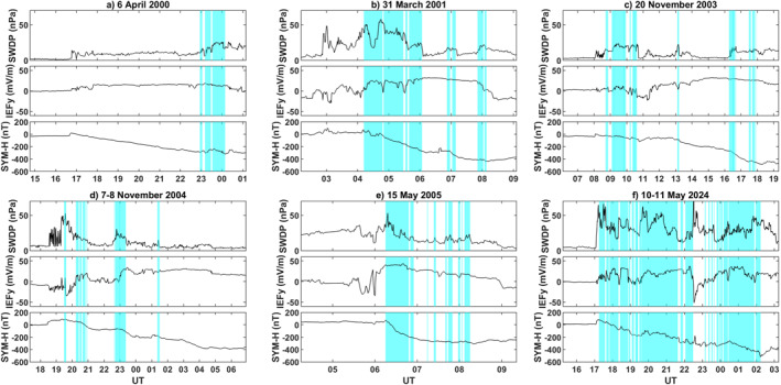
Comparison of most intense storms with peak negative Sym‐H less than −300 nT occurred during solar cycles 23–25 along with the present storm. Shaded region indicates the periods with SWDP ≥ 15 nPa simultaneously with IEFY ≥ 2.5 mV/m [refer text and Table‐1 for more details].
Table‐1 presents a comparison of peak negative Sym‐H (Sym‐H peak), the total decrease of Sym‐H during the main phase (Sym‐H range), main phase duration, duration with IEFY ≥ 2.5 mV/m, and duration with a combination of SWDP ≥ 15 nPa and IEFY ≥ 2.5 mV/m for all six storms depicted in Figure 6. The storms are listed in the order of Sym‐H range (total decrease in Sym‐H during the main phase). It is clear that the longer high SWDP (≥15 nPa) and IEFY (≥2.5 mV/m) conditions, the larger Sym‐H range, which was −606 nT during the present storm, and the Sym‐H ranges systematically decrease with the reduction in the durations of these conditions. On the other hand, the duration of IEFY ≥ 2.5 mV/m alone does not show any systematic variation with the Sym‐H range.
Table 1.
Comparison of Most Intense Storms That Occurred in Solar Cycles 23–25
| Dates | SYM‐H peak | SYM‐H range | Main phase duration | Duration with IEFy ≥ 2.5 (mV/M) | Duration with SWDP ≥ 15 (nPa) and IEFy ≥ 2.5 (mV/M) |
|---|---|---|---|---|---|
| 10 May 2024 | −518 | −606 | 539 | 444 | 409 |
| 31 Mar 2001 | −437 | −512 | 235 | 228 | 132 |
| 20 Nov 2003 | −490 | −498 | 612 | 496 | 79 |
| 7 Nov 2004 | −394 | −489 | 635 | 512 | 78 |
| 15 May 2005 | −305 | −377 | 125 | 125 | 68 |
| 6 Apr 2000 | −320 | −339 | 445 | 441 | 54 |
Figure 7 displays a bar diagram of Sym‐H ranges as a function of duration (in minutes) that satisfies the conditions of IEFY ≥ 2.5 mV/m alone (top panel) and the combination of SWDP ≥ 15 nPa and IEFY ≥ 2.5 mV/m (bottom panel). From the top panel, it is evident that conditions of IEFY ≥ 2.5 mV/m alone cannot explain the variation of Sym‐H ranges. For example, the condition IEFY ≥ 2.5 mV/m was sustained for nearly similar durations on 6 April 2000 (441 min) and 10–11 May 2024 (444 min) storms. However, weaker SWDP conditions on 6 April 2000 (see Figure 6a) limited the Sym‐H range only to −339 nT. On the other hand, stronger SWDP conditions caused a large Sym‐H range of −606 nT in the present storm. It may also be noted here that although the IEFY ≥ 2.5 mV/m was sustained for nearly 441, the magnitude of IEFY was slightly due to smaller solar wind velocity (not shown in figure) during the 6 April 2000 storm compared to that of the 10–11 May 2024 storm. The smaller levels of IEFY would also be partly responsible for the reduced Sym‐H range during the 6 April 2000 storm besides the weaker SWDP conditions.
Figure 7.
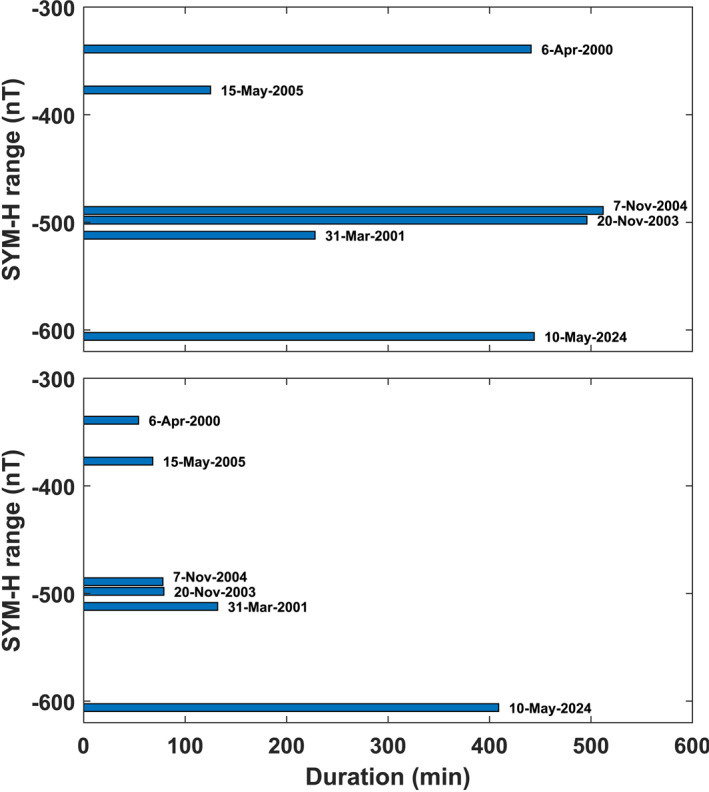
Sym‐H ranges as a function of durations (in minutes) under the conditions of IEFY ≥ 2.5 mV/m alone (top panel) and the combination of SWDP ≥ 15 nPa and IEFY ≥ 2.5 mV/m (bottom panel).
From the bottom panel of Figure 7, it can be clearly seen that the combination of SWDP ≥ 15 nPa and IEFY ≥ 2.5 mV/m better explains the variation in Sym‐H ranges. The Sym‐H range increases systematically with the longer durations of SWDP ≥ 15 nPa and IEFY ≥ 2.5 mV/m. Therefore, from the results presented in Figures 4, 5, 6, 7 and Table 1, we conclude that the sustenance of high SWDP simultaneously with eastward IEFY (≥2.5 mV/m) for nearly 409 min was the key factor responsible for this super‐intense storm with a total Sym‐H range of −606 nT. As discussed above, the potent combination of high SWDP and intense eastward IEFY would cause a strong ring current guided to flow at much closer distances to Earth, leading to strong magnetic field disturbances on the ground.
3.2. Impacts Observed in the Ionosphere
Strong electrodynamical disturbances triggered via enhanced solar wind—magnetosphere ‐ ionosphere interactions during this geomagnetic storm led to severe ionospheric total electron content (TEC) disturbances and a strong positive storm lasted for several hours on the dayside ionosphere. Figure 8 shows the global TEC maps during the main phase of the storm (middle panels) compared with the previous day (9 May 2024, top panels). It is clearly observed that the TEC on 10 May 2024 was dramatically enhanced over American longitudes (dayside) with more than a 100% increase compared to the previous quiet day. In the bottom panels are shown the latitudinal variations of TEC over the American (75oW) sector. Strong enhancements in TEC can be seen from low to mid‐latitudes (up to ±45°) in both hemispheres due to enhanced Equatorial Ionization Anomaly (EIA). Further, the crests of the EIA appear to have shifted significantly poleward on 10 May 2024 compared to those on 09 May 2024. This suggests that strong eastward penetration electric fields (PPEF) prevailed over the equatorial latitudes, leading to the strong equatorial fountain effect and an intensified EIA during this period (Tsurutani et al., 2004; Mannucci et al., 2005; Tulasi Ram et al., 2008, 2019; Venkatesh et al., 2017). In addition to the eastward PPEF, the enhanced equatorward neutral wind driven by Joule and particle heating at high latitudes also causes the uplifting of F‐layer via inclined magnetic field lines at mid‐latitudes (Fuller‐Rowell et al., 1994; Balan et al., 2009, 2012). The combined effects of the intensified equatorial fountain effect via PPEF and the enhanced equatorward neutral wind uplift the F‐region to the altitudes of reduced recombination, leading to such a strong positive ionospheric storm as seen in Figure 8. It may be recalled that one unit of TEC variation can cause an error of upto 0.16 m in positioning by single‐frequency GPS receiver (for example, Øvstedal, 2002], which are most commonly used for navigation by the majority of civilians. Therefore, the strong enhancements in TEC can lead to severe errors in positioning/navigation based on single‐frequency GPS receivers. Significant degradations in GPS‐based positional accuracy were also reported during this storm, affecting agricultural and drone users (Koebler, 2024; Davis, 2024).
Figure 8.
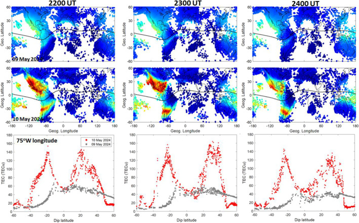
Global ionospheric TEC maps on 09th (top panels) and 10th May 2024 (bottom panels) showing the TEC enhancements with more than 100% on dayside ionosphere. Bottom panels show the latitudinal distribution of TEC along the American (75°W) longitudinal indicating the intensified Equatorial Ionization Anomaly (EIA).
The strong X‐class solar flare (X3.9 in Figure 1), which peaked at 0654 UT on 10 May 2024 (before the storm), was also found to have severely affected HF radio waves over the Indian sector. Figures 9a–9c depict the variations of X‐ray solar flux from the GOES satellite, VLF signal amplitude measured at 19.8 kHz using an NWC receiver, and the Equatorial Electrojet (EEJ) strength. Here, EEJ is computed using the two‐station method from the H‐component observations measured at an equatorial (Tirunelveli) and off‐equatorial (Alibag) pair of magnetometers (Rastogi, 1977; Reddy, 1989; Tulasi Ram et al., 2024) from the Indian sector. The blue curves represent the variation on 10 May 2024 and the black curves represent the variation on a previous quiet day (9 May 2024). It can be seen from these figures that both the VLF signal amplitude (a proxy to the D‐region ionization) and the EEJ strength (a proxy to the E‐region ionization) increased in tandem with the increase in the X‐ray flux. This suggests that the enhanced X‐ray flux due to this solar flare led to a significantly increased photoionization in the D‐ and E‐regions of the ionosphere over the Indian sector. The right‐hand side panels (Figures 9d–9i) present the ionograms obtained from a digital ionosonde at the Indian equatorial station, Tirunelveli. This figure shows that the ionogram traces were completely absent from 0,640 to 0700 UT and became very faint from 0,700 to 0720 UT. This indicates that the radiowaves were absorbed by intense ionization in the D‐ and E‐regions, caused by this solar flare, resulting in a radio blackout in the 2–12 MHz frequency band.
Figure 9.
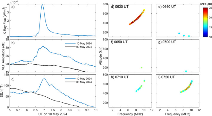
(a–c) UT variations of X‐Ray flux (top), VLF amplitude (middle) and Equatorial Electrojet (EEJ, bottom) during the X3.9 solar flare around 0654 UT (d–i) Ionograms observed from the Indian equatorial station, Tirunelveli from 0630 to 0720 UT. The absence of ionogram traces from 0640 to 0710 UT indicates the radio blackout due to the absorption of radio waves from 2 to 12 MHz.
4. Summary and Conclusions
A series of Solar flares and Coronal Mass Ejections (CMEs) occurred from 8 to 9 May 2024, interacted with one another on their voyage toward Earth, and formed a composite ICME that impacted Earth's magnetosphere around 1705 UT on tenth May 2024. At least two distinct ICMEs can be identified within this ICME, which reached the L1‐point at 1634 UT and 2136 UT. The corresponding shock signatures in ground‐based magnetometers were observed at 1705 UT and 2221 UT. The globally averaged surface geomagnetic field (Sym‐H index) was depressed by 518 nT, making it the most intense geomagnetic storm of the past three decades and the second‐largest in the space era (in terms of Sym‐H index). The strong SWDP associated with this composite ICME caused Earth's dayside magnetopause to be pushed below the geostationary orbit (6.6 R E) for continuously ∼6 hr. Furthermore, the Earth's magnetospheric bow shock was also found to compress below the geostationary orbit for about 3 min. The BATSRUS model simulations suggest that the magnetopause location could have been as low as 3.3 R E during the peak phase of the storm. Our study further reveals that a potent combination of high SWDP (≥15 nPa) with intense eastward IEFY (≥2.5 mV/m) that lasted for 409 min is the key factor responsible for the development of a strong ring current at much closer to the Earth, making this storm uniquely intense. Severe electrodynamic disturbances caused strong eastward PPEFs, significantly intensified EIA, and large SED (>100%) in the dayside ionosphere, which can severely affect the positioning/navigation based on single‐frequency GPS receivers. The enhanced D‐ and E‐region ionization due to an X3.9 solar flare at ∼0654 UT caused the absorption of radio waves in the range 2–12 MHz, resulting in an HF radio blackout over the Indian sector.
Supporting information
Supporting Information S1
Acknowledgments
The authors acknowledge the open data policy of NASA's DSCOVR and GOES‐18 data products. We also acknowledge NASA's SPDF for the solar wind and the Madrigal database at Millstone Hill for worldwide GNSS‐TEC data products. The WDC, Kyoto University is acknowledged for Sym‐H index data. We acknowledge CCMC for facilitating MHD model simulations and Dr. B. Nilam for her help in running the BATSRUS model on CCMC. We also thank Ms. M. Ankita for her help in analyzing and plotting the figures. We also thank Mr. Siba Kiran Guru for his help in plotting ionograms.
Tulasi Ram, S. , Veenadhari, B. , Dimri, A. P. , Bulusu, J. , Bagiya, M. , Gurubaran, S. , et al. (2024). Super‐intense geomagnetic storm on 10–11 May 2024: Possible mechanisms and impacts. Space Weather, 22, e2024SW004126. 10.1029/2024SW004126
Contributor Information
S. Tulasi Ram, Email: tulasiram.s@iigm.res.in.
A. P. Dimri, Email: apdimri@hotmail.com.
Data Availability Statement
The DSCOVR solar wind and IMF data are available at https://www.ngdc.noaa.gov/dscovr/portal/index.html#/download/. The Sym‐H index data is obtained from the World Data Center for Geomagnetism, Kyoto University (Imajo et al., 2022). The magnetic field (Bz and By) data from the GOES‐18 satellite at 10 Hz resolution are downloaded from https://cdaweb.gsfc.nasa.gov/pub/data/goes/goes18/. The TEC map data from the worldwide GNSS receiver network are downloaded from the Madrigal database at Millstone Hill (http://millstonehill.haystack.mit.edu/listExperiments?isGlobal=on&categories=17&instruments=8000&showDefault=on&start_date_0=1950‐01‐01&start_date_1=00%3A00%3A00&end_date_0=2024‐12‐31&end_date_1=23%3A59%3A59). The SWDP, IMF Bz and Sym‐H data of past geomagnetic storms are obtained from Omni web interface of NASA's Space Physics Data Facility (https://omniweb.gsfc.nasa.gov/form/omni_min_def.html). All the data from magnetometers, VLF receivers, and Ionosonde operated by IIG are made available at the public data repository (IIG, 2024). The 1‐min Dst (equivalent to Sym‐H index) and the closest magnetopause location (LMP) data from the BATSRUS model run are available at the Community Coordinate Modeling Center (CCMC). https://ccmc.gsfc.nasa.gov/results/viewrun.php?runnumber=Nilam_Bhosale_071124_1.
References
- Akasofu, S. I. (1980). The solar wind‐magnetosphere energy coupling and magnetospheric disturbances. Planetary and Space Science, 28(5), 495–509. 10.1016/0032-0633(80)90031-8 [DOI] [Google Scholar]
- Akasofu, S. I. , Chapman, S. , & Venkatesan, D. (1963). The main phase of great magnetic storms. Journal of Geophysical Research, 68(11), 3345–3350. 10.1029/JZ068i011p03345 [DOI] [Google Scholar]
- Araki, T. (1977). Global structure of geomagnetic sudden commencements. Planetary and Space Science, 25(4), 373–384. 10.1016/0032-0633(77)90053-8 [DOI] [Google Scholar]
- Balan, N. , Liu, J. Y. , Otsuka, Y. , Tulasi Ram, S. , & Lühr, H. (2012). Ionospheric and thermospheric storms at equatorial latitudes observed by CHAMP, ROCSAT, and DMSP. Journal of Geophysical Research, 117(A1), A01313. 10.1029/2011JA016903 [DOI] [Google Scholar]
- Balan, N. , Shiokawa, K. , Otsuka, Y. , Watanabe, S. , & Bailey, G. J. (2009). Super plasma fountain and equatorial ionization anomaly during penetration electric field. Journal of Geophysical Research, 114, A03310. 10.1029/2008JA013768 [DOI] [Google Scholar]
- Burlaga, L. F. , Fitzenreiter, R. , Lepping, R. , Ogilvie, K. , Szabo, A. , Lazarus, A. , et al. (1998). A magnetic cloud containing prominence material: January 1997. Journal of Geophysical Research, 103(A1), 277–285. 10.1029/97ja02768 [DOI] [Google Scholar]
- Burlaga, L. F. , Klein, L. , Sheeley, N. R. , Michels, D. J. , Howard, R. A. , Koomen, M. J. , et al. (1982). A magnetic cloud and a coronal mass ejection. Geophysical Research Letters, 9(12), 1317–1320. 10.1029/gl009i012p01317 [DOI] [Google Scholar]
- Burton, R. K. , McPherron, R. L. , & Russell, C. T. (1975). An empirical relationship between interplanetary conditions and Dst. Journal of Geophysical Research, 80(31), 4204–4214. 10.1029/JA080i031p04204 [DOI] [Google Scholar]
- Daglis, I. A. , Thorne, R. M. , Baumjohann, W. , & Orsini, S. (1999). The terrestrial ring current: Origin, formation, and decay. Review of Geophysics, 37(4), 407–438. 10.1029/1999RG900009 [DOI] [Google Scholar]
- Davis, W. (2024). Solar Storms are disrupting farmer GPS systems during critical planting time. Verge. https://www.theverge.com/2024/5/12/24154779/solar‐storms‐farmer‐gps‐john‐deer [Google Scholar]
- Dungey, J. W. (1961). Interplanetary magnetic field and the auroral zones. Physical Review Letters, 6(2), 47–48. 10.1103/PhysRevLett.6.47 [DOI] [Google Scholar]
- Fuller‐Rowell, T. J. , Codrescu, M. V. , Moffett, R. J. , & Quegan, S. (1994). Response of the thermosphere and ionosphere to geomagnetic storms. Journal of Geophysical Research, 99(A3), 3893–3914. 10.1029/93ja02015 [DOI] [Google Scholar]
- Gonzalez, W. , & B. Tsurutani, B. (1987). Criteria of interplanetary parameters causing intense magnetic storms (Dst< −100 nT). Planetary and Space Science, 35(9), 1101–1109. 10.1016/0032-0633(87)90015-8 [DOI] [Google Scholar]
- Gonzalez, W. D. , Echer, E. , Gonzalez, A. , Tsurutani, B. T. , & Dal Lago, A. (2011). Interplanetary origin of intense, superintense and extreme geomagnetic storms. Space Science Reviews, 158(1), 69–89. 10.1007/s11214-010-9715-2 [DOI] [Google Scholar]
- Gopalswamy, N. (2006). Properties of interplanetary coronal mass ejections. Space Science Reviews, 124(1–4), 145–168. 10.1007/s11214-006-9102-1 [DOI] [Google Scholar]
- Grandin, M. , Bruus, E. , Ledvina, V. E. , Partamies, N. , Barthelemy, M. , Martinis, C. , et al. (2024). The geomagnetic superstorm of 10 May 2024. Citizen science observations, EGUsphere [preprint]. 10.5194/egusphere-2024-2174 [DOI]
- Harel, M. , Wolf, R. A. , Reiff, P. H. , Spiro, R. W. , Burke, W. J. , Rich, F. J. , & Smiddy, M. (1981). Quantitative simulation of a magnetospheric substorm 1, Model logic and overview. Journal of Geophysical Research, 86(A4), 2217–2241. 10.1029/ja086ia04p02217 [DOI] [Google Scholar]
- Hayakawa, H. , Ebihara, Y. , Mishev, A. , Koldobskiy, S. , Kusano, K. , Bechet, S. , et al. (2024). The solar and geomagnetic storms in may 2024: A flash data report. arXiv preprint. 10.48550/arXiv.2407.07665 [DOI] [Google Scholar]
- Holzer, R. E. , & Slavin, J. A. (1978). Magnetic flux transfer associated with expansions and contractions of the dayside magnetosphere. Journal of Geophysical Research, 83(A8), 3831–3839. 10.1029/JA083iA08p03831 [DOI] [Google Scholar]
- IIG . (2024). Magnetometer and ionospheric observations from Indian sector during 10‐11 may 2024 storm [Dataset]. Zenodo. 10.5281/zenodo.12623351 [DOI]
- Imajo, S. , Matsuoka, A. , Toh, H. , & Iyemori, T. (2022). Mid‐latitude geomagnetic indices ASY and SYM (ASY/SYM indices). World Data Center for Geomagnetism. 10.14989/267216 [DOI] [Google Scholar]
- Iyemori, T. , Araki, T. , Kamei, T. , & Takeda, M. (1992). Mid‐latitude geomagnetic indices ASY and SYM (provisional). Data Analysis Center for Geomagnetism and Space Magnetism, Faculty of Science, Kyoto University. [Google Scholar]
- Kilpua, E. , Koskinen, H. E. , & Pulkkinen, T. I. (2017). Coronal mass ejections and their sheath regions in interplanetary space. Living Reviews in Solar Physics, 14, 1–83. 10.1007/s41116-017-0009-6 [DOI] [PMC free article] [PubMed] [Google Scholar]
- Koebler, J. (2024). Solar storm knocks out farmers' tractor GPS systems during peak planting season. https://www.404media.co/solar‐storm‐knocks‐out‐tractor‐gps‐systems‐during‐peak‐planting‐season/
- Lepping, R. P. , Burlaga, L. F. , Szabo, A. , Ogilvie, K. W. , Mish, W. H. , Vassiliadis, D. , et al. (1997). The Wind magnetic cloud and events of October 18–20, 1995: Interplanetary properties and as triggers for geomagnetic activity. Journal of Geophysical Research, 102(A7), 14049–14064. 10.1029/97ja00272 [DOI] [Google Scholar]
- Liemohn, M. , Ganushkina, N. Y. , De Zeeuw, D. L. , Rastaetter, L. , Kuznetsova, M. , Welling, D. T. , et al. (2018). Real‐time SWMF at CCMC: Assessing the Dst output from continuous operational simulations. Space Weather, 16(10), 1583–1603. 10.1029/2018SW001953 [DOI] [Google Scholar]
- Liu, Y. D. , Chen, C. , & Zhao, X. (2020). Characteristics and importance of “ICME in‐sheath” phenomenon and upper limit for geomagnetic storm activity. The Astrophysical Journal Letters, 897(1), L11. 10.3847/2041-8213/ab9d25 [DOI] [Google Scholar]
- Lohrey, B. , & Kaiser, A. B. (1979). Whistler‐induced anomalies in VLF propagation. Journal of Geophysical Research, 84(A9), 5121–5130. 10.1029/ja084ia09p05122 [DOI] [Google Scholar]
- Loto'aniu, P. T. M. , Romich, K. , Rowland, W. , Codrescu, S. , Biesecker, D. , Johnson, J. , et al. (2022). Validation of the DSCOVR spacecraft mission space weather solar wind products. Space Weather, 20(10), e2022SW003085. 10.1029/2022SW003085 [DOI] [Google Scholar]
- Macdougall, J. , Grant, I. , & Shen, X. (1995). The Canadian advanced digital ionosonde: Design and results. [S.l.], report UAG‐14: Ionospheric networks and stations. World Data Center A for Solar‐Terrestrial Physics, 21–27. [Google Scholar]
- Machol, J. L. , Eparvier, F. G. , Viereck, R. A. , Woodraska, D. L. , Snow, M. , Thiemann, E. , et al. (2020). GOES‐R series solar X‐ray and ultraviolet irradiance. In The GOES‐R series (pp. 233–242). Elsevier. [Google Scholar]
- Maezawa, K. (1974). Dependence of the magnetopause position on the southward interplanetary magnetic field. Planetary and Space Science, 22(10), 1443–1453. 10.1016/0032-0633(74)90040-3 [DOI] [Google Scholar]
- Mannucci, A. J. , Tsurutani, B. T. , Iijima, B. A. , Komjathy, A. , Saito, Gonzalez, A. , Gonzalez, W. D. , et al. (2005). Dayside global ionospheric response to the major interplanetary events of October 29–30, 2003 “Halloween Storms”. Geophysical Research Letters, 32(12). 10.1029/2004GL021467 [DOI] [Google Scholar]
- Newell, S. , Liou, M. , Liou, K. , Meng, C. , & Rich, F. J. (2007). A nearly universal solar wind‐magnetosphere coupling function inferred from 10 magnetospheric state variables. Journal of Geophysical Research, 112(1), 1–16. 10.1029/2006JA012015 [DOI] [Google Scholar]
- Ober, D. M. , Thomsen, M. F. , & Maynard, N. C. (2002). Observations of bow shock and magnetopause crossings from geosynchronous orbit on 31 March 2001. Journal of Geophysical Research, 107(A8), SMP–27. 10.1029/2001JA000284 [DOI] [Google Scholar]
- O'Brien, T. , & McPherron, R. L. (2000). Forecasting the ring current index Dst in real time. Journal of Atmospheric and Solar‐Terrestrial Physics, 62(14), 1295–1299. 10.1016/s1364-6826(00)00072-9 [DOI] [Google Scholar]
- Øvstedal, O. (2002). Absolute positioning with single‐frequency GPS receivers. GPS Solutions, 5(4), 33–44. 10.1007/PL00012910 [DOI] [Google Scholar]
- Powell, K. , Roe, P. , Linde, T. , Gombosi, T. , & De Zeeuw, D. L. (1999). A solution‐adaptive upwind scheme for ideal magnetohydrodynamics. Journal of Computational Physics, 154(2), 284–309. 10.1006/jcph.1999.6299 [DOI] [Google Scholar]
- Rastogi, R. G. (1977). Geomagnetic storms and electric fields in the equatorial ionosphere. Nature, 268(5619), 422–424. 10.1038/268422a0 [DOI] [Google Scholar]
- Rastogi, R. G. , Janardhan, P. , Chandra, H. , Trivedi, N. B. , & Erick, V. (2017). Effect of solar flare on the equatorial electrojet in eastern Brazil region. Journal of Earth System Science, 126(4), 51. 10.1007/s12040-017-0837-8 [DOI] [Google Scholar]
- Rastogi, R. G. , Pathan, B. M. , Rao, D. R. K. , Sastry, T. S. , & Sastri, J. H. (1999). Solar flare effects on the geomagnetic elements during normal and counter electrojet periods. Earth Planets and Space, 51(9), 947–957. 10.1186/bf03351565 [DOI] [Google Scholar]
- Reddy, C. A. (1989). The equatorial electrojet. Pure and Applied Geophysics, 131(3), 485–508. 10.1007/bf00876841 [DOI] [Google Scholar]
- Ridley, A. J. , Gombosi, T. I. , & De Zeeuw, D. L. (2004). Ionospheric control of themagnetosphere: Conductance. Annales Geophysicae, 22(2), 567–584. 10.5194/angeo-22-567-2004 [DOI] [Google Scholar]
- Sibeck, D. G. , Lopez, R. E. , & Roleof, E. C. (1991). Solar wind control of the magnetopause shape, location, and motion. Journal of Geophysical Research, 96(A4), 5489–5495. 10.1029/90JA02464 [DOI] [Google Scholar]
- Sripathi, S. , Balachandran, N. , Veenadhari, B. , Singh, R. , & Emperumal, K. (2013). Response of the equatorial and low‐latitude ionosphere to an intense X‐class solar flare (X7/2B) as observed on 09 August 2011. Journal of Geophysical Research: Space Physics, 118(5), 2648–2659. 10.1002/jgra.50267 [DOI] [Google Scholar]
- Sugiura, M. (1991). Equatorial Dst index 1957‐1986. IAGA Bulletin, 40, 17–38. [Google Scholar]
- Temmer, M. , & Bothmer, V. (2022). Characteristics and evolution of sheath and leading edge structures of interplanetary coronal mass ejections in the inner heliosphere based on Helios and Parker Solar Probe observations. Astronomy and Astrophysics, 665, A70. 10.1051/0004-6361/202243291 [DOI] [Google Scholar]
- Toffoletto, F. , Sazykin, S. , Spiro, R. , & Wolf, R. (2003). Inner magnetospheric modeling with the Rice convection model. Space Science Reviews, 107(1/2), 175–196. 10.1007/978-94-007-1069-6_19 [DOI] [Google Scholar]
- Tsurutani, B. T. , Mannucci, A. , Iijima, B. , Abdu, M. A. , Sobral, J. H. A. , Gonzalez, W. , et al. (2004). Global dayside ionospheric uplift and enhancement associated with interplanetary electric fields. Journal of Geophysical Research, 109(A8), A08302. 10.1029/2003JA010342 [DOI] [Google Scholar]
- Tulasi Ram, S. , Ankita, M. , Nilam, B. , Gurubaran, S. , Nair, M. , Seemala, G. K. , et al. (2024). Empirical model of Equatorial ElectroJet (EEJ) using long‐term observations from the Indian sector. Space Weather, 22(7), e2024SW003988. 10.1029/2024SW003988 [DOI] [Google Scholar]
- Tulasi Ram, S. , Nilam, B. , Balan, N. , Zhang, Q. , Shiokawa, K. , Chakrabarty, D. , et al. (2019). Three different episodes of prompt equatorial electric field perturbations under steady southward IMF Bz during St. Patrick's Day storm. Journal of Geophysical Research: Space Physics, 124(12), 10428–10443. 10.1029/2019JA027069 [DOI] [Google Scholar]
- Tulasi Ram, S. , Rama Rao, P. V. S. , Prasad, D. S. V. V. D. , Niranjan, K. , Gopi Krishna, S. , Sridharan, R. , & Sudha, R. (2008). Local time dependent response of postsunset ESF during geomagnetic storms. Journal of Geophysical Research, 113(A7). 10.1029/2007JA012922 [DOI] [Google Scholar]
- Vallat, C. , Dandouras, I. , Dunlop, M. , Balogh, A. , Lucek, E. , Parks, G. K. , et al. (2005). First current density measurements in the ring current region using simultaneous multi‐spacecraft CLUSTER‐FGM data. Annales Geophysicae, 23(5), 1849–1865. 10.5194/angeo-23-1849-2005 [DOI] [Google Scholar]
- Venkatesh, K. , Tulasi Ram, S. , Fagundes, P. R. , Seemala, G. K. , & Batista, I. S. (2017). Electrodynamic disturbances in the Brazilian equatorial and low‐latitude ionosphere on St. Patrick's Day storm of 17 March 2015. Journal of Geophysical Research: Space Physics, 122(4), 4553–4570. 10.1002/2017JA024009 [DOI] [Google Scholar]
- Xia, Z. , Chen, L. , Zhima, Z. , & Parrot, M. (2020). Spectral broadening of NWC transmitter signals in the ionosphere. Geophysical Research Letters, 47(13), e2020GL088103. 10.1029/2020GL088103 [DOI] [Google Scholar]
- Yu, Y. , Ridley, A. J. , Welling, D. T. , & Tóth, G. (2010). Including gap region field‐aligned currents and magnetospheric currents in the MHD calculation of ground‐based magnetic field perturbations. Journal of Geophysical Research, 115(A8), A08207. 10.1029/2009JA014869 [DOI] [Google Scholar]
Associated Data
This section collects any data citations, data availability statements, or supplementary materials included in this article.
Data Citations
- Grandin, M. , Bruus, E. , Ledvina, V. E. , Partamies, N. , Barthelemy, M. , Martinis, C. , et al. (2024). The geomagnetic superstorm of 10 May 2024. Citizen science observations, EGUsphere [preprint]. 10.5194/egusphere-2024-2174 [DOI]
- IIG . (2024). Magnetometer and ionospheric observations from Indian sector during 10‐11 may 2024 storm [Dataset]. Zenodo. 10.5281/zenodo.12623351 [DOI]
Supplementary Materials
Supporting Information S1
Data Availability Statement
The DSCOVR solar wind and IMF data are available at https://www.ngdc.noaa.gov/dscovr/portal/index.html#/download/. The Sym‐H index data is obtained from the World Data Center for Geomagnetism, Kyoto University (Imajo et al., 2022). The magnetic field (Bz and By) data from the GOES‐18 satellite at 10 Hz resolution are downloaded from https://cdaweb.gsfc.nasa.gov/pub/data/goes/goes18/. The TEC map data from the worldwide GNSS receiver network are downloaded from the Madrigal database at Millstone Hill (http://millstonehill.haystack.mit.edu/listExperiments?isGlobal=on&categories=17&instruments=8000&showDefault=on&start_date_0=1950‐01‐01&start_date_1=00%3A00%3A00&end_date_0=2024‐12‐31&end_date_1=23%3A59%3A59). The SWDP, IMF Bz and Sym‐H data of past geomagnetic storms are obtained from Omni web interface of NASA's Space Physics Data Facility (https://omniweb.gsfc.nasa.gov/form/omni_min_def.html). All the data from magnetometers, VLF receivers, and Ionosonde operated by IIG are made available at the public data repository (IIG, 2024). The 1‐min Dst (equivalent to Sym‐H index) and the closest magnetopause location (LMP) data from the BATSRUS model run are available at the Community Coordinate Modeling Center (CCMC). https://ccmc.gsfc.nasa.gov/results/viewrun.php?runnumber=Nilam_Bhosale_071124_1.