The effect of resampling techniques on the performances of machine learning clinical risk prediction models in the setting of severe class imbalance: development and internal validation in a retrospective cohort

Abstract

Purpose

The availability of population datasets and machine learning techniques heralded a new era of sophisticated prediction models involving a large number of routinely collected variables. However, severe class imbalance in clinical datasets is a major challenge. The aim of this study is to investigate the impact of commonly-used resampling techniques in combination with commonly-used machine learning algorithms in a clinical dataset, to determine whether combination(s) of these approaches improve upon the original multivariable logistic regression with no resampling.

Methods

We previously developed and internally validated a multivariable logistic regression 30-day mortality prediction model in 30,619 patients using preoperative and intraoperative features.

Using the same dataset, we systematically evaluated and compared model performances after application of resampling techniques [random under-sampling, near miss under-sampling, random oversampling, and synthetic minority oversampling (SMOTE)] in combination with machine learning algorithms (logistic regression, elastic net, decision trees, random forest, and extreme gradient boosting).

Results

We found that in the setting of severe class imbalance, the impact of resampling techniques on model performance varied by the machine learning algorithm and the evaluation metric. Existing resampling techniques did not meaningfully improve area under receiving operating curve (AUROC). The area under the precision recall curve (AUPRC) was only increased by random under-sampling and SMOTE for decision trees, and oversampling and SMOTE for extreme gradient boosting. Importantly, some combinations of algorithm and resampling technique decreased AUROC and AUPRC compared to no resampling.

Conclusion

Existing resampling techniques had a variable impact on models, depending on the algorithms and the evaluation metrics. Future research is needed to improve predictive performances in the setting of severe class imbalance.

Introduction

Every year, more than 300 million surgeries are performed globally, with more than 4 million deaths [1]. Worldwide, postoperative mortality is the third leading cause of death, after ischaemic heart disease and stroke, contributing to 8% of all deaths [1]. There has been significant research interest in the accurate prediction of postoperative mortality, to assist with perioperative risk stratification, shared decision making, and disposition planning [2–8]. The availability of population perioperative datasets from electronic health record (EHR) [9] and machine learning techniques heralded a new era of sophisticated prediction models. These models involve a large number of routinely collected preoperative and intraoperative variables, such as demographics, surgery types, laboratory values, and vital signs [5, 7, 8]. However, a major challenge in postoperative mortality prediction is the problem of severe class imbalance in the clinical datasets [10].

Class imbalance occurs when the event rate of a binary outcome (i.e. has two categories or classes) is <50% and can be particularly problematic when the outcome is rare [10, 11]. In the setting of postoperative mortality prediction, the incidence of mortality is typically 2% or lower [3, 5–8]. Such extreme class imbalance poses two significant challenges during model development and validation. First, during model development, the algorithms will mostly learn from samples without events. Second, standard performance metrics [e.g. accuracy and area under receiving operating curve (AUROC)] can be misleading and overly optimistic in the setting of class imbalance [10–12]. For example, with a mortality event rate of only 2%, a model that predicts that no one dies will only be wrong only 2% of the time and will be correct 98% of the time. However, such a model would be useless and harmful, despite high accuracy. Moreover, clinicians are more interested in predicting who will have the event in order to implement appropriate interventions (such as increased monitoring). Thus, missing a high-risk patient may lead to dire consequences.

Several methods have been used in the literature to mitigate the issue of imbalanced datasets [10, 11], which can be grouped into the broad categories performance metrics and resampling techniques. In terms of performance metrics, several alternatives have been studied [13]. The area under precision-recall curve (AUPRC) presents precision [positive predictive value (PPV)] against recall (sensitivity) and indicates how well the model  can predict true positives [12]. The baseline of AUPRC in a given model is the event rate in the dataset [12]. However, this metric has only been reported in two papers in the postoperative mortality prediction literature [7, 8]. In terms of model development, a possible approach involves using resampling techniques in the derivation set [7, 14, 15], to balance the class distribution by sampling more from patients with events (over-sampling) or sampling less from patients without events (under-sampling). Note that resampling is never applied to the validation set, such that model performances can be correctly calculated in a dataset with the unaltered, real-life event rate.

However, it remains under active research how different resampling techniques to improve class imbalance affect model performances when used in combination with machine learning algorithms (learners), which would be important to inform best practices in clinical machine learning modeling. While studies found that resampling techniques improved model performances, the effectiveness of the resampling strategies varies with the dataset and the learner [16, 17]. As within a given dataset it is usually unknown which one will have the best performance, one must also test multiple learners for the domain task under consideration. Special-purpose algorithms have been proposed to learn in conditions where the data is imbalanced, such as different versions of extreme gradient boosting (XGBoost) [18, 19]. Moreover, some characteristics of medical data, such as high dimensionality, can lead to problems that can make resampling strategies less effective in improving model performance [18, 19].

We have previously developed and internally validated a multivariable logistic regression 30-day mortality prediction model in 30,619 patients using preoperative and intraoperative features, with validation set AUROC of 0.893 (95% CI 0.861–0.920) and AUPRC of 0.158 (baseline 0.017 based on mortality rate) [8]. The aim of this study is to systematically evaluate and compare commonly-used resampling techniques [random under-sampling, near miss under-sampling, random oversampling, and synthetic minority oversampling (SMOTE)] in combination with commonly-used machine learning algorithms (logistic regression, elastic net, decision trees, random forest, and extreme gradient boosting) in a clinical dataset where the events are rare, to determine whether combination(s) of these approaches improve upon the original multivariable logistic regression with no resampling.

Materials and methods

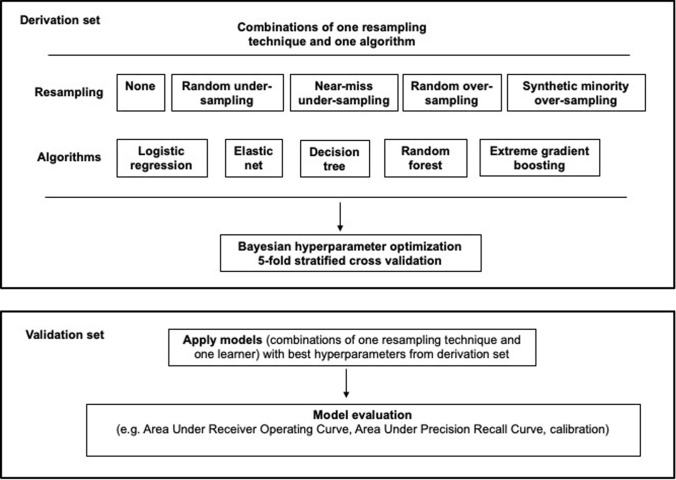
We received research ethics approval (Nova Scotia Health Authority Research Ethics Board, Halifax, NS, Canada; file # 1024251), with waiver informed consent for secondary analysis of de-identified population dataset developed in a published retrospective cohort study [8]. Figure 1 illustrates the methodology of this study.

Fig. 1.

Methodology overview

Dataset

Please see the previous publication [8] for details about the dataset. Briefly, the cohort consists of 30,619 patients age ≥45 and undergoing inpatient noncardiac surgery (except deceased organ donation) at two tertiary academic hospitals in Halifax, Nova Scotia, Canada, between January 1, 2013 to December 1, 2017. Multiple sources of data [hospitals’ Anesthesia Information Management System (AIMS) containing intraoperative vital signs and anesthetic interventions, hospitals’ perioperative EHR, the Nova Scotia Vital Statistics database which documented all deaths within Nova Scotia, and Canadian Institute for Health Information (CIHI) Discharge Abstract Database (DAD)] were linked to create the final de-identified dataset containing preoperative, intraoperative, and postoperative variables. The final de-identified dataset was extracted by and accessed through Health Data Nova Scotia (HDNS).

To mirror real-life application, where prediction models are built using data from the past and validated with prospective data, the cohort was divided into derivation and validation sets temporally by ranking surgery dates from the earliest to the latest [8]. The derivation set consisted of patients with the earliest 75% of the surgery dates, and the validation set consisted of patients with the latest 25% of the surgery dates (i.e. 75:25 division). There were no major differences in cohort characteristics between the derivation and validation datasets (standardized mean difference were all <0.2) [8].

Also, the models in this study used the same final set of features (predictors) and event (outcome) as the previously published primary multivariable logistic regression model [8]. The event was all-cause mortality within 30 days after surgery, in- or out-of-hospital. The event rate was 2.2% (493/22964) in the derivation set, and 1.7% (131/7655) in the validation set (i.e., the derivation and validation sets have an imbalance ratio of 2.2 and 1.7%, respectively). While the class imbalance ratios within the derivation and validation sets are extremely high, they are within the expected values observed in the literature for postoperative mortality, where the typical imbalance ratio is approximately 2% or lower. The features (predictors) are listed in Table 1. The mean (SD) age was 66 (11) years, with 50.2% female (8).

Table 1 .

List of features according to preoperative, intraoperative vital signs, and other intraoperative groups

Features
Preoperative features
Age (years)
Female sex
Emergency surgery
Procedural Index for Mortality Risk
Surgery type (compared to general surgery)
Neurosurgery
Obstetrics and gynecology
Orthopedic surgery
Other
Otolaryngology
Plastic surgery
Thoracic surgery
Urology
Vascular surgery
Hypertension
Chronic obstructive pulmonary disease
Revised Cardiac Risk Index
Elixhauser Comorbidity Index
Hospital Frailty Risk Score
Obesity
Vital signs features
Max. decrease (%) of SBP relative to first AIMS SBP
Cumulative duration (minutes) < MAP 70 mmHg
Max. change of HR in 10 BPM above first AIMS HR
Max. change of HR in 10 BPM below first AIMS HR
Cumulative duration (minutes) of HR < 60
Cumulative duration (minutes) of HR > 100
Cumulative duration (minutes) SpO2 < 88%
Cumulative duration (hour) of temperature <36 °C
Cumulative duration (hour) of temperature >38 °C
Cumulative duration (minutes) ETCO2 < 30 mmHg, GA
Cumulative duration (minutes) of ETCO2 > 45 mmHg, GA
Other intraoperative features
Duration of Surgery (hour)
General anesthesia
Neuraxial anesthesia
Peripheral nerve block
Laparoscopic surgery with no conversion to open
Age-adjusted MAC during GA, time averaged
Crystalloid (L) above 1L
Use of vasopressors and inotropes
Use of vasodilators

For the surgery type, the reference group was general surgery

AIMS Anesthesia Information Management System, BPM beats per minute, ETCO₂ end-tidal CO₂, GA general anesthesia, HR heart rate, IQR interquartile range, MAC Minimal Alveolar Concentration, MAP mean arterial pressure, Max. maximum, SE standard error, SBP systolic blood pressure

Statistical analysis

Software

Data analysis was performed on the HDNS Citadel server using R 4.1.0 and Python 2.7.10 (in particular scikit-learn, hyperopt, and imblearn) [20–23].

Pre-processing

To facilitate machine learning, one hot encoding was used for categorical encoding, and standard scaling was applied to continuous variables with zero mean and unit standard deviation.

Resampling techniques

The resampling approaches tested were: no resampling, random under-sampling [24, 25], near miss under-sampling [26], random oversampling [24, 25], and SMOTE [10, 11]. The more frequent event class (i.e. patients without mortality in our dataset) is referred to as the majority class, and the less frequent event class (i.e. patients with mortality in our dataset) the minority class. The class weight and resampling ratio are amongst hyperparameter that needed to be tuned (please see “Hyperparameter tuning” below). Under-sampling addresses class imbalance by removing samples from the majority class randomly (random under-sampling) or by proximity in the feature distribution space amongst majority and minority classes (near-miss under-sampling). Over-sampling balances the dataset by adding subjects to the minority class with randomly selected replicas (random over-sampling) or by generating sample data by interpolating amongst randomly selected subjects and their K nearest neighbours (SMOTE) [27, 28].

Machine learning algorithms

The algorithms developed in the derivation set were logistic regression, elastic net [29], decision tree [30], random forest [31], and XGBoost [32]. Elastic net is logistic regression with L1 and L2 regularization, which helps reduce overfitting. Decision trees are simple models that are interpretable. XGBoost and random forest are ensemble methods based on decision trees, which work well for nonlinear relationships, can reveal feature importance, and help reduce overfitting.

Hyperparameter optimization

Each algorithm has hyperparameters that must be optimized (Appendix 1). Hyperparameter tuning for algorithms, class weight, and the resampling ratio are necessary to ensure that when comparing the different models, the differences are due to the algorithm or the resampling technique rather than suboptimal hyperparameter settings. In the derivation set, Bayesian optimization [22, 33] was used to efficiently obtain the best hyperparameters for each model, with five-fold stratified cross validation in the derivation set using AUROC as the metric. The models were subsequently validated in the validation set using the best hyperparameters.

Model validation

Model performances were evaluated in the validation set. A variety of metrics were calculated, since no single metric is sufficient for discerning the best model [34, 35]. The main metrics assessed were AUROC (95% CI calculated by 2000 stratified bootstrap replicates using the original event rate in the test set) and AUPRC.

In addition, sensitivity (also known as recall), specificity, positive predictive value (also known as precision), negative predictive value, F1-score (harmonic mean of precision and recall, i.e. measure of accuracy), and G-mean (geometric mean of sensitivity and specificity, helpful in imbalanced datasets) were assessed at a probability threshold of 0.5.

Results

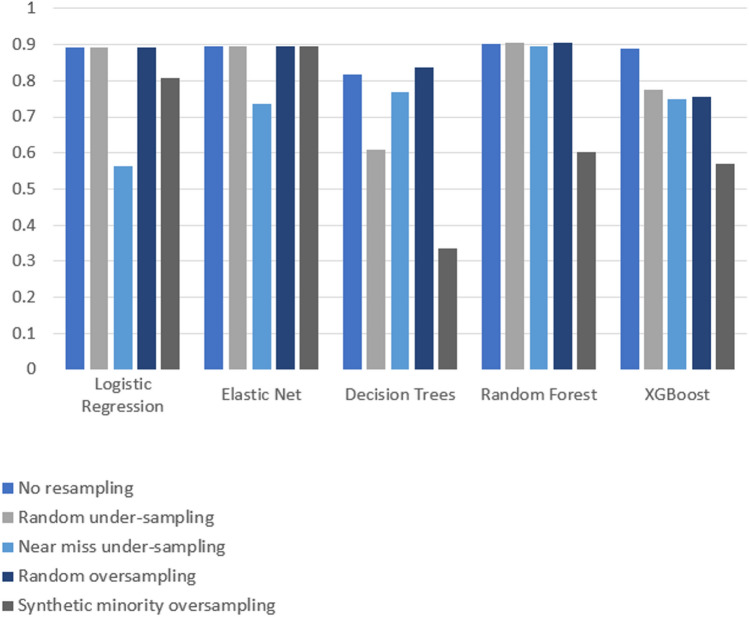
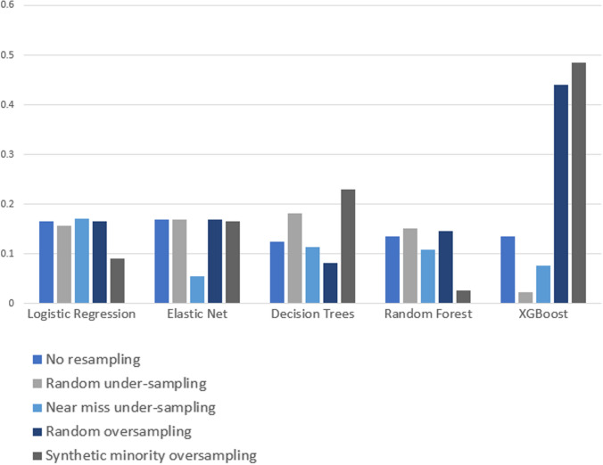
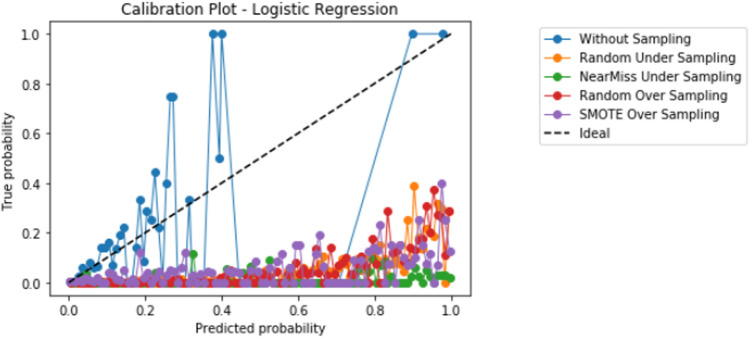
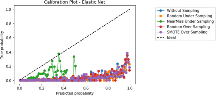
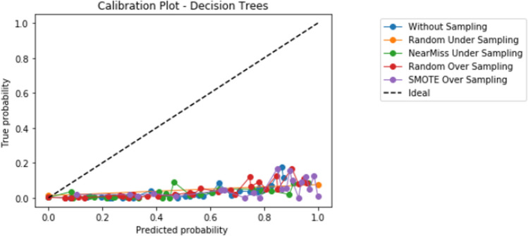
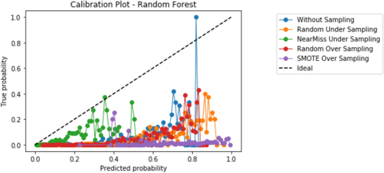
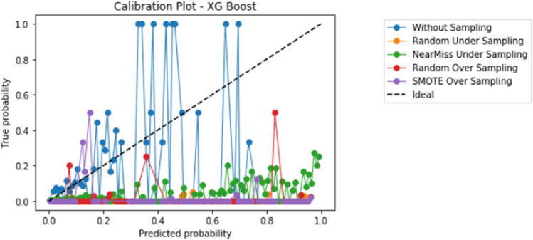
Compared to logistic regression, at baseline (without resampling), the other models (elastic net, decision tree, random forest, and XGBoost) did not meaningfully improve upon the AUROC nor AUPRCs. Different resampling techniques impacted each algorithm differently. A summary of the performances from combinations of each resampling technique and each algorithm are displayed in Fig. 2 for AUROC, and Fig. 3 for AUPRC. Importantly, despite the high AUROC, all models exhibited poor calibration (Appendix 2).

Fig. 2.

Area under the receiver operating curve (AUROC) results from combinations of algorithms and resampling techniques. Legend: y-axis, area under the receiver operating curve (AUROC); x-axis, algorithms in combination with resampling techniques

Fig. 3.

Area under the precision recall curve (AUPRC) results from combinations of algorithms and resampling techniques. Legend: y-axis, area under the precision recall curve (AUPRC); x-axis, algorithms in combination with resampling techniques

Overall, existing resampling techniques improved some performance metrics (i.e. AUPRC) for decision tree and XGBoost, but did not meaningfully improve model performances for logistic regression, elastic net, and random forest. Random over-sampling minimally improved AUROC for decision trees (0.837 with over-sampling vs. 0.817 without resampling), though this needs to be interpreted in the context of lower baseline AUROC compared to other algorithms. The AUPRC was only increased by random under-sampling and SMOTE for decision trees (increase between 0.05 and 0.1, approximately), and oversampling and SMOTE for XGBoost (increase between 0.3 and 0.35, approximately).

Importantly, some combinations of algorithm and resampling technique decreased AUROC and AUPRC compared to no resampling. For example, all resampling techniques returned worse AUROC for XGBoost (with a decrease ranging between 0.1 and 0.3), and near miss undersampling decreased the AUROC of logistic regression (approximately 0.3 decrease) and elastic net (approximately 0.15 decrease). For AUPRC, SMOTE decreased AUPRC for logistic regression, and random forest (approximately 0.1 decrease), while near miss undersampling decreased the AUPRC for elastic net, randomforest, and XGBoost (decrease ranging between 0.05 and 0.1). Overall, the AUROC bootstrapped results show a performance consistent with the non-bootstrapped results for all learning algorithms and resampling techniques. The exception to this is a general decrease in performance for the alternative of not using any resampling technique. This decrease ranged between approximately 0.1 for elastic net, decision trees, and random forest, to a 0.4 decrease for XGBoost. When using logistic regression with the option involving no resampling, a performance of approximately 0.9 is observed for both bootstrapped and non-bootstrapped alternatives.

The performances of the five algorithms in combination with each resampling approach are displayed in Table 2 (no resampling), Table 3 (random under-sampling), Table 4 (near-miss under-sampling), Table 5 (random over-sampling), and Table 6 (SMOTE). Table 7 provides the p-values of a paired t-test carried out for each learning algorithm comparing pairs of resampling techniques, on both AUROC and AUPRC scores, with the Benjamini–Hochberg correction [39] for multiple hypothesis testing.

Table 2.

Model performances in the validation set for algorithms with no resampling

Metric	Logistic regression	Elastic net	Decision trees	Random forest	XGBoost
AUROC	0.892	0.897	0.817	0.903	0.888
Bootstrapped AUROC mean	0.890	0.733	0.702	0.777	0.485
Bootstrapped AUROC 95% CI	0.859–0.918	0.698–0.769	0.657–0.749	0.743–0.809	0.436–0.537
AUPRC	0.166	0.169	0.125	0.135	0.135
Precision	0.400	0.074	0.040	0.111	0.166
Recall (sensitivity)	0.015	0.853	0.830	0.700	0.030
F1-score	0.030	0.136	0.080	0.190	0.051
Specificity	0.999	0.816	0.962	0.903	0.997
Negative predictive value	0.980	0.996	0.995	0.994	0.983
Geometric mean	0.124	0.834	0.752	0.795	0.175

Bootstrapping was performed using 2000 replicates

AUROC area under the receiver operating curve, AUPRC area under the precision recall curve, CI confidence interval

Table 3.

Model performances in the validation set for algorithms with random under-sampling

Algorithm	Logistic regression	Elastic net	Decision trees	Random forest	XGBoost
AUROC	0.893	0.895	0.609	0.906	0.775
Bootstrapped AUROC mean	0.897	0.897	0.609	0.906	0.775
Bootstrapped AUROC 95% CI	0.871–0.923	0.870–0.923	0.573–0.648	0.880–0.930	0.747–0.800
AUPRC	0.157	0.169	0.182	0.151	0.022
Precision	0.080	0.071	0.070	0.089	0.020
Recall	0.823	0.838	0.270	0.861	0.961
F1-score	0.145	0.132	0.118	0.161	0.040
Specificity	0.836	0.813	0.941	0.847	0.261
Negative predictive value	0.996	0.996	0.986	0.997	0.997
Geometric mean	0.829	0.825	0.510	0.845	0.501

Bootstrapping was performed using 2000 replicates

AUROC area under the receiver operating curve, AUPRC area under the precision recall curve, CI confidence interval

Table 4.

Model performances in the validation set for algorithms with near-miss under-sampling

Algorithm	Logistic regression	Elastic net	Decision trees	Random forest	XGBoost
AUROC	0.564	0.737	0.767	0.894	0.750
Bootstrapped AUROC mean	0.564	0.738	0.767	0.894	0.750
Bootstrapped AUROC 95% CI	0.518–0.611	0.699–0.778	0.729–0.805	0.868–0.918	0.727–0.780
AUPRC	0.171	0.055	0.114	0.109	0.077
Precision	0.018	0.029	0.040	0.125	0.150
Recall	0.923	0.815	0.715	0.007	0.084
F1-score	0.037	0.057	0.070	0.014	0.100
Specificity	0.175	0.541	0.704	0.999	0.980
Negative predictive value	0.992	0.994	0.993	0.983	0.990
Geometric mean	0.402	0.664	0.710	0.087	0.380

Bootstrapping was performed using 2000 replicates

AUROC area under the receiver operating curve, AUPRC area under the precision recall curve, CI confidence interval

Table 5.

Model performances in the validation set for algorithms with random over-sampling

Metric	Logistic regression	Elastic net	Decision trees	Random forest	XGBoost
AUROC	0.892	0.895	0.837	0.906	0.756
Bootstrapped AUROC mean	0.893	0.895	0.727	0.906	0.754
Bootstrapped AUROC 95% CI	0.863–0.920	0.866–0.921	0.687–0.767	0.881–0.928	0.718–0.786
AUPRC	0.166	0.169	0.082	0.146	0.441
Precision	0.080	0.074	0.051	0.080	0.017
Recall	0.800	0.838	0.776	0.800	0.946
F1-score	0.154	0.136	0.105	0.158	0.030
Specificity	0.845	0.818	0.785	0.856	0.104
Negative predictive value	0.996	0.996	0.992	0.995	0.990
Geometric mean	0.826	0.828	0.775	0.827	0.314

Bootstrapping was performed using 2000 replicates

AUROC area under the receiver operating curve, AUPRC area under the precision recall curve, CI confidence interval

Table 6.

Model performances in the validation set for algorithms with synthetic minority oversampling technique (SMOTE)

Algorithm	Logistic regression	Elastic net	Decision trees	Random forest	XGBoost
AUROC	0.808	0.895	0.334	0.604	0.570
Bootstrapped AUROC mean	0.808	0.895	0.334	0.603	0.578
Bootstrapped AUROC 95% CI	0.769–0.845	0.866–0.922	0.291–0.375	0.554–0.657	0.555–0.598
AUPRC	0.091	0.166	0.229	0.026	0.484
Precision	0.078	0.075	0.010	0.016	0.017
Recall	0.423	0.838	0.923	0.976	0.969
F1-score	0.132	0.138	0.03	0.032	0.034
Specificity	0.913	0.821	0.077	0.008	0.058
Negative predictive value	0.989	0.996	0.983	0.955	0.990
Geometric mean	0.621	0.830	0.266	0.090	0.237

Bootstrapping was performed using 2000 replicates

AUROC area under the receiver operating curve, AUPRC area under the precision recall curve, CI confidence interval

Table 7.

P-value results of a paired t-test comparing all resampling techniques for each learner with the Benjamini–Hochberg correction [39]

Learners	Resampling	AUROC				AUPRC
		SMOTE	RUS	ROS	NearM	SMOTE	RUS	ROS	NearM
Decision trees	Baseline	0.0000	0.0000	0.0065	0.0000	0.0000	0.0000	0.0000	0.0309
	SMOTE		0.0000	0.0000	0.0000		0.0000	0.0000	0.0000
	RUS			0.0000	0.0000			0.0000	0.0000
	ROS				0.0000				0.0002
ElasticNet	Baseline	0.8285	0.8230	0.5734	0.0000	0.2968	0.9682	0.9682	0.0000
	SMOTE		0.8592	0.8592	0.0000		0.2968	0.2206	0.0000
	RUS			0.8285	0.0000			0.9755	0.0000
	ROS				0.0000				0.0000
Logistic regression	Baseline	0.0000	0.3181	0.2290	0.0000	0.0000	0.0882	0.0520	0.0933
	SMOTE		0.0000	0.0000	0.0000		0.0000	0.0000	0.0000
	RUS			0.5566	0.0000			0.0260	0.0238
	ROS				0.0000				0.0816
Random forest	Baseline	0.0000	0.7833	0.1926	0.0304	0.0000	0.0043	0.0692	0.0000
	SMOTE		0.0000	0.0000	0.0000		0.0000	0.0000	0.0030
	RUS			0.3952	0.0086			0.0030	0.0000
	ROS				0.0133				0.0000
XGBoost	Baseline	0.0000	0.0000	0.0000	0.0000	0.0000	0.0000	0.0000	0.0000
	SMOTE		0.0000	0.0000	0.0000		0.0000	0.0000	0.0000
	RUS			0.0000	0.0007			0.0000	0.0000
	ROS				0.9138				0.0000

AUROC area under the receiver operating curve, AUPRC area under the precision recall curve, NearM near miss under-sampling, ROS random oversampling, RUS random under-sampling, SMOTE synthetic minority oversampling

Discussion

In medical settings, prediction models must be able to accurately identify which patients will have rare but severe consequences, such as postoperative mortality. However, model performances are often overestimated by commonly reported metrics such as the AUROC [12]. It remains unknown the optimal approaches to improve the models’ ability to identify positive cases in the setting of severe class imbalance. Our study systematically evaluated the performances of combinations of algorithms and resampling techniques in a highly imbalanced cohort with imbalance ratios of 2.2% and 1.7% in the derivation and validation sets, respectively. This study found that in the setting of severe class imbalance, the impact of resampling techniques on model performance varied by the machine learning algorithm and the evaluation metric, and that existing resampling techniques are inadequate to meaningfully improve model performances. With the exception of decision trees and XGBoost, the resampling techniques worsened or only minimally improved AUROC or AUPRC. For decision trees, random oversampling minimally improved AUROC, while random under-sampling and SMOTE improved AUPRC. For XGBoost, random oversampling and SMOTE increased AUPRC but at the cost of decreased AUROC. Some combinations of algorithm and resampling techniques worsened model performance.

The overall poor results of AUROC may indicate that the dataset have other factors that were not solved by resampling techniques. The loss in performance observed when applying near miss under-sampling when compared to random under-sampling points to the presence of other factors such as small disjuncts not directly related to the imbalance that are not addressed by these techniques. Moreover, the performance loss observed for all learners when applying SMOTE indicates that in this case at least one of the known scenarios that cause SMOTE to fail is present (e.g. small disjuncts, presence of outliers). Regarding the AUPRC results, the same impact in performance is observed with the exception of random under-sampling and SMOTE for decision trees, and random oversampling and SMOTE for XGBoost. Still, these improvements are obtained in a setting where all alternatives exhibit a very low performance (below 0.2). Overall, this shows that the predictive task involves other more complex factors that resampling techniques generally are not able to address.

Importantly, despite high AUROC, all models demonstrated poor calibration. The additional impact of different techniques to improve calibration in combination with resampling techniques and learners, including Platt scaling, isotonic regression, or Bayesian binning into quantiles, should also be further explored in future studies. Our study highlights that further research is much needed to develop techniques to improve prediction in the setting of severe class imbalance that is common in many medical applications of machine learning [10]. When modeling using a dataset with class imbalance, researchers may consider exploring a variety of resampling techniques in combination with different algorithms.

Our results align with the findings from a recent study by van den Goorbergh et al. [36]. They examined model performances of standard and penalized logistic regression models in the setting of under-sampling, over-sampling, and SMOTE, in a dataset of 3369 patients with an event rate of 20%. They also performed Monte Carlo simulations of various numbers of predictors and outcome event rates. They found that resampling methods did not improve AUROC and worsened calibration, though they did not examine AUPRC. Rather than changing event distribution, van den Goorbergh et al. suggest refining the probability threshold for classifying events from non-events. Finding the optimal probability threshold may be difficult in practice in the clinical setting, as we need to balance the consequences of not applying interventions on patients with events versus unnecessarily treating patients with non-events. We agree with van den Goorbergh et al. that a decision curve analysis approach focusing on Net Benefit [37] may be complementary for optimizing clinical utility.

Other studies using medical data suggest that resampling techniques effectively improve performance [16]. However, how resampling strategies impact performance is not well understood, especially in the setting of factors specific to individual datasets such as small disjuncts that may hinder the performance of resampling techniques and add complexity to the predictive task [11]. Problems intrinsic to the resampling techniques have also been identified. For instance, in high-dimensional datasets, issues with SMOTE includes decrease in the variability of the minority class or the introduction of correlation between some samples [38]. Our results align with these difficulties, except for XGBoost when observing the AUPRC. Regarding the performance of the XGBoost, mixed results have been reported regarding its capability to deal with imbalanced data [18]. Our results align with the literature that XGBoost impacts performance differently depending on the metric and resampling techniques are applied.

Regarding paired t-tests of model performances with the Benjamini–Hochberg correction [39] for multiple hypothesis testing (Table 7), all decision tree results are statistically significant for AUROC and AUPRC (p-values <0.05). The same trend is observed for XGBoost (p-values <0.05) with the exception of the pair random oversampling and near miss for AUROC which has a high p-value. For elastic net, both metrics do not show statistically significant results for all resampling techniques pairs except for the pairs involving near miss. In this case, when compared against near miss, all alternative resampling strategies tested show a p-value >0.22, while the pairs including near miss show a p-value <0.05. Finally, a more mixed scenario is observed for random forest and logistic regression where generally no statistical significance is observed with the exception of pairs involving SMOTE on both metrics (exhibiting a p-value <0.05) and pairs involving near miss for AUCROC (with a p-value <0.05 for both models) or most pairs involving random under-sampling for AUPRC (all pairs show a p-value <0.05, except the random undersampling and baseline pair for which the logistic regression model shows a p-value of ~0.0882).

In addition to model performances, the computational efficiency, memory usage, and complexity of the models in the setting of electronic health records and healthcare informatics networks must also be considered. Overall, logistic regression and elastic net may be more resource efficient, while random forest and the XGBoost are the most time-consuming. When considering the resampling techniques, both under-sampling techniques (random unders-sampling and near miss under-sampling) reduce the dataset size and in turn learner training time and memory usage, but present the risk of information loss. Random oversampling and SMOTE have a high memory usage and increase the dataset size, which leads to a higher training time for the learners.

Strengths and limitations

The strengths of our study include a robust clinical dataset with large sample size and high data quality, systematic evaluation of combinations of algorithms and resampling techniques, and use of Bayesian hyperparameter tuning to ensure hyperparameter optimization of the models. Our conclusions are limited by the use of a retrospective dataset from tertiary academic hospitals, and prospective, external validation are required. Moreover, the machine learning algorithms used are restricted to logistic and decision tree-based models. Other types of machine learning models should be considered in the future. This study considered all features available in the original model [8] (Table 1), and no additional feature selection method was applied beyond the learner; the impact of feature selection in conjunction with resampling can be explored as future research. Our study focused on the most used resampling techniques, and the impact in performance of more advanced resampling techniques under highly imbalanced settings can be further explored. We observed an overall poor calibration of the algorithms, an issue that should be addressed in future research through methods such as Platt scaling or isotonic regression. Finally, our results are dependent on the dataset used and might not be generalizable to other dataset in the medical domain or other applications. Simulation studies can help better understand the characteristics of the resampling methods that are dependent and independent of the datasets used to improve generalizability.

Conclusion

This study found that in the setting of severe class imbalance, the impact of resampling techniques on model performance varied by the machine learning algorithm and the evaluation metric. Existing resampling techniques did not meaningfully improve model performances for logistic regression, elastic net, and random forest. For XGBoost, improvements in AUPRC random oversampling and SMOTE were offset by decreased AUROC. Performances of decision trees were improved by multiple resampling techniques.

Future research is needed to improve predictive performances in the setting of severe class imbalance.

Appendix

Appendix 1: Hyperparameter optimization

Elastic net

Hyperparameter	Range of Parameter tested	No resampling	Resampling strategy
			Random under-sampling	Near miss under-sampling	Random oversampling	Synthetic minority oversampling
C	1 to 1000, increment of 10	800	140	130	10	130
Class weight	None, Balanced	Balanced	None	Balanced	Balanced	Balanced
L1 ratio	0.1 to 0.9, increment of 0.1	0.5	0.4	0.2	0.7	0.2
Max Iteration	1000 to 100,000	2606	91,357	91,323	36,888	91,232
Sampling Strategy	0.1 to 0.9, increment of 0.1	N/A	0.2	0.1	0.2	0.1

Decision trees

Hyperparameter	Range of parameter tested	No resampling	Resampling strategy
			Random under-sampling	Near miss under-sampling	Random oversampling	Synthetic minority oversampling
Maximum depth	5 to 70, increment of 1	39	41	41	50	10
Maximum features	Sqrt, Log2	Sqrt	Sqrt	Sqrt	Log2	Sqrt
Criterion	Gini, Entropy	Gini	Entropy	Entropy	Entropy	Entropy
Class weight	Balanced, None	Balanced	Balanced	Balanced	Balanced	Balanced
Minimum samples leaf	1, 100, 200, 300, 400, 500	300	100	100	4000	200
Sampling Strategy	0.1 to 0.9, increment of 0.1	N/A	0.1	0.1	0.4	0.6

Random forest

Hyperparameter	Range of parameter tested	No resampling	Resampling strategy
			Random under-sampling	Near miss under-sampling	Random oversampling	Synthetic minority oversampling
Class weight	None, Balanced	Balanced	Balanced	Balanced	Balanced	Balanced
Criterion	Entropy, GINI	GINI	Entropy	Entropy	Entropy	Entropy
Max depth	6 to 15	7	13	14	6	14
Max features	Sqrt, Log2	Log2	Sqrt	Sqrt	Sqrt	Sqrt
Number of estimators	100 to 1000	972	604	630	460	630
Sampling strategy	0.1 to 0.9, increment of 0.1	N/A	0.8	0.3	0.6	0.4

XGBoost

Hyperparameter	Range of parameter tested	No resampling	Resampling strategy
			Random under-sampling	Near miss under-sampling	Random oversampling	Synthetic minority oversampling
Gamma	0 to 0.5, increment of 0.01	0.47	0.42	0.11	0.49	0.49
Learning rate	0 to 0.5, increment of 0.01	0.07	0.11	0.33	0.09	0.09
Max depth	5 to 70, increment of 1	38	10	25	9	9
Minimum child weight	1 to 10, increment of 1	10	7	8.0	1	1.0
Number of Estimators	20–200, 5	16	20	20	28	28
Scale positive weight	1 or 91,454 (ratio of positive to negative classes from training set)	1	91,454	1	91,454	91,454
Sampling Strategy	0.1 to 0.9, increment of 0.1	N/A	0.1	0.1	0.1	0.1

Appendix 2: Calibration graphs

Appendix 2.1 Logistic regression

Appendix 2.2 Elastic net

Appendix 2.3 Decision tree

Appendix 2.4 Random forest

Appendix 2.5 XGBoost

Author contributions

JK: Study design, data analysis, interpretation, manuscript first draft and revisions. AD: Study design, data analysis, interpretation, manuscript first draft and revisions. PB: Study design, data analysis, interpretation, manuscript revisions. RG: Study design, interpretation, manuscript revisions.

Funding

Natural Sciences and Engineering Research Council of Canada for open access publication fees. Department of Anesthesia, Pain Management & Perioperative Medicine at Dalhousie University ($2,595) and Nova Scotia Health Authority Research Fund ($5000) for the previously published cohort dataset (https://doi.org/10.1007/s12630-022-02287-0).

Data availability

The datasets used in this study are managed by the Health Data Nova Scotia and Nova Scotia Health Authority, and are not publicly available due to provincial privacy legislation and institutional restrictions. Analysis codes are available here: Dakshinamurthy A. GitHub In hospital Mortality Prediction Research Project [Internet]. 2022 [cited 2022 Sep 8]. Available from: https://github.com/Arunachalam4505/In-hospital-Mortality-Prediction-Research-Project.

Disclaimer

The data used in this report were made available by Health Data Nova Scotia of Dalhousie University. Although this research analysis is based on data obtained from the Nova Scotia Department of Health and Wellness, the observations and opinions expressed are those of the authors and do not represent those of either Health Data Nova Scotia or the Department of Health and Wellness.

Declarations

Ethics approval and consent to participate

We obtained research ethics approval (Nova Scotia Health Authority Research Ethics Board, Halifax, NS, Canada; file # 1024251), and conducted this study according to the principles of the Declaration of Helsinki.

Competing interests

Dr. Janny Ke received salary support as the Clinical Data Lead, St. Paul’s Hospital, Canada, for Project “Reducing Opioid Use for Pain Management” from Canadian Digital Supercluster DIGITAL and Consortium (Careteam Technologies Inc, Thrive Health Inc, Excelar Technologies (Connected Displays Inc), Providence Health Care Ventures Inc, and Xerus Inc). Dr Ke provided paid consulting for Careflow Technologies (Connected Displays Inc), funded via Providence Health Care Ventures. Dr. Ke receives research and salary support for Project "Continuous Connected Patient Care" in patients with high perioperative risk, funded by DIGITAL and Consortium: Medtronic Canada ULC, Cloud Diagnostics Canada ULC, Excelar Technologies (Connected Displays Inc), Providence Health Care Ventures Inc, 3D Bridge Solutions Inc, and FluidAI (NERv Technology Inc). Dr. Paula Branco received research funding from NSERC, Mitacs, IBM and University of Ottawa.

References

- 1.Nepogodiev D, et al. Global burden of postoperative death. Lancet. 2019;393(10170):401. [DOI] [PubMed] [Google Scholar]
- 2.Moonesinghe SR, Mythen MG, Das P, Rowan KM, Grocott MPW. Risk stratification tools for predicting morbidity and mortality in adult patients undergoing major surgery: qualitative systematic review. Anesthesiology. 2013;119(4):959–81. [DOI] [PubMed] [Google Scholar]
- 3.Wong DJN, Harris S, Sahni A, Bedford JR, Cortes L, Shawyer R, et al. Developing and validating subjective and objective risk-assessment measures for predicting mortality after major surgery: an international prospective cohort study. PLOS Med. 2020;17(10): e1003253. [DOI] [PMC free article] [PubMed] [Google Scholar]
- 4.Sigakis MJG, Bittner EA, Wanderer JP. Validation of a risk stratification index and risk quantification index for predicting patient outcomesin-hospital mortality, 30-day mortality, 1-year mortality, and length-of-stay. Anesthesiol J Am Soc Anesthesiol. 2013;119(3):525–40. [DOI] [PubMed] [Google Scholar]
- 5.Lee CK, Hofer I, Gabel E, Baldi P, Cannesson M. Development and validation of a deep neural network model for prediction of postoperative in-hospital mortality. Anesthesiology. 2018;129(4):649–62. [DOI] [PMC free article] [PubMed] [Google Scholar]
- 6.Hill BL, Brown R, Gabel E, Rakocz N, Lee C, Cannesson M, et al. An automated machine learning-based model predicts postoperative mortality using readily-extractable preoperative electronic health record data. Br J Anaesth. 2019;123(6):877–86. [DOI] [PMC free article] [PubMed] [Google Scholar]
- 7.Fritz BA, Cui Z, Zhang M, He Y, Chen Y, Kronzer A, et al. Deep-learning model for predicting 30-day postoperative mortality. Br J Anaesth. 2019;123(5):688–95. [DOI] [PMC free article] [PubMed] [Google Scholar]
- 8.Ke JXC, McIsaac DI, George RB, Branco P, Cook EF, Beattie WS, et al. Postoperative mortality risk prediction that incorporates intraoperative vital signs: development and internal validation in a historical cohort. Can J Anesth. 2022. 10.1007/s12630-022-02287-0. [DOI] [PubMed] [Google Scholar]
- 9.Kazemi P, Lau F, Simpao AF, Williams RJ, Matava C. The state of adoption of anesthesia information management systems in Canadian academic anesthesia departments: a survey. Can J Anaesth J Can Anesth [Internet]. 2021 Jan 29; Available from: https://rdcu.be/cesb5 [DOI] [PubMed]
- 10.Megahed FM, Chen YJ, Megahed A, Ong Y, Altman N, Krzywinski M. The class imbalance problem. Nat Methods. 2021;18(11):1270–2. [DOI] [PubMed] [Google Scholar]
- 11.Branco P, Torgo L, Ribeiro RP. A survey of predictive modeling on imbalanced domains. ACM Comput Surv. 2016;49(2):31:1-31:50. [Google Scholar]
- 12.Saito T, Rehmsmeier M. The precision-recall plot is more informative than the ROC plot when evaluating binary classifiers on imbalanced datasets. PLoS ONE. 2015;10(3): e0118432. [DOI] [PMC free article] [PubMed] [Google Scholar]
- 13.Gaudreault JG, Branco P, Gama J. An analysis of performance metrics for imbalanced classification. In: Soares C, Torgo L, editors. Discovery science: lecture notes in computer science. Cham: Springer International Publishing; 2021. p. 67–77. [Google Scholar]
- 14.Brajer N, Cozzi B, Gao M, Nichols M, Revoir M, Balu S, et al. Prospective and external evaluation of a machine learning model to predict in-hospital mortality of adults at time of admission. JAMA Netw Open. 2020;3(2): e1920733. [DOI] [PubMed] [Google Scholar]
- 15.Davoodi R, Moradi MH. Mortality prediction in intensive care units (ICUs) using a deep rule-based fuzzy classifier. J Biomed Inform. 2018;79:48–59. [DOI] [PubMed] [Google Scholar]
- 16.Kabir MF, Ludwig S. Classification of Breast Cancer Risk Factors Using Several Resampling Approaches. In: 2018 17th IEEE International Conference on Machine Learning and Applications (ICMLA) [Internet]. 2018 [cited 2024 Sep 22]. p. 1243–8. Available from: https://ieeexplore.ieee.org/document/8614227
- 17.Khushi M, Shaukat K, Alam TM, Hameed IA, Uddin S, Luo S, et al. A comparative performance analysis of data resampling methods on imbalance medical data. IEEE Access. 2021;9:109960–75. [Google Scholar]
- 18.Wang C, Deng C, Wang S. Imbalance-XGBoost: leveraging weighted and focal losses for binary label-imbalanced classification with XGBoost. Pattern Recognit Lett. 2020;1(136):190–7. [Google Scholar]
- 19.Zhang P, Jia Y, Shang Y. Research and application of XGBoost in imbalanced data. Int J Distrib Sens Netw. 2022;18(6):15501329221106936. [Google Scholar]
- 20.Dakshinamurthy A. GitHub In hospital Mortality Prediction Research Project [Internet]. 2022 [cited 2022 Sep 8]. Available from: https://github.com/Arunachalam4505/In-hospital-Mortality-Prediction-Research-Project
- 21.scikit-learn: machine learning in Python—scikit-learn 1.1.2 documentation [Internet]. [cited 2022 Sep 8]. Available from: https://scikit-learn.org/stable/
- 22.Bergstra J, Yamins D, Cox DD. Making a science of model search: hyperparameter optimization in hundreds of dimensions for vision architectures. In: Proceedings of the 30th International Conference on International Conference on Machine Learning - Volume 28. Atlanta, GA. JMLR.org; 2013. p. I-115–I-123. (ICML’13).
- 23.imbalanced-learn documentation—Version 0.9.1 [Internet]. [cited 2022 Sep 8]. Available from: https://imbalanced-learn.org/stable/
- 24.Kubat M, Matwin S. Addressing the curse of imbalanced training sets: one-sided selection. Fourteenth Int Conf Mach Learn. 1997;97(1):1–8. [Google Scholar]
- 25.Estabrooks A, Jo T, Japkowicz N. A multiple resampling method for learning from imbalanced data sets. Comput Intell. 2004;20(1):18–36. [Google Scholar]
- 26.Zhang J, Mani I. KNN approach to unbalanced data distributions: a case study involving information extraction. In: Proceedings of the ICML’2003 Workshop on Learning from Imbalanced Datasets; 2003.
- 27.Chawla NV, Bowyer KW, Hall LO, Kegelmeyer WP. SMOTE: synthetic minority over-sampling technique. J Artif Intell Res. 2002;16(1):321–57. [Google Scholar]
- 28.Fernandez A, Garcia S, Herrera F, Chawla NV. SMOTE for learning from imbalanced data: progress and challenges, marking the 15-year anniversary. J Artif Intell Res. 2018;20(61):863–905. [Google Scholar]
- 29.Zou H, Hastie T. Regularization and variable selection via the elastic net. J R Stat Soc Ser B Stat Methodol. 2005;67(2):301–20. [Google Scholar]
- 30.Breiman L, Friedman JH, Olshen RA, Stone CJ. Classification and regression trees. Monterey, CA: Wadsworth and Brooks; 1984. [Google Scholar]
- 31.Breiman L. Random forests. Mach Learn. 2001;45(1):5–32. [Google Scholar]
- 32.Chen T, Guestrin C. XGBoost: A scalable tree boosting system. Proc 22nd ACM SIGKDD Int Conf Knowl Discov Data Min. 2016.
- 33.Pelikan M, Goldberg DE, Cantú-Paz E. BOA: the Bayesian optimization algorithm. In: Proceedings of the 1st Annual Conference on Genetic and Evolutionary Computation - Volume 1. San Francisco, CA: Morgan Kaufmann Publishers Inc.; 1999. p. 525–32. (GECCO’99).
- 34.James G, Witten D, Hastie T, Tibshirani R. An introduction to statistical learning: with applications in R. Springer texts in statistics. New York: Springer; 2013. [Google Scholar]
- 35.Steyerberg EW, Vickers AJ, Cook NR, Gerds T, Gonen M, Obuchowski N, et al. Assessing the performance of prediction models: a framework for some traditional and novel measures. Epidemiol Camb Mass. 2010;21(1):128–38. [DOI] [PMC free article] [PubMed] [Google Scholar]
- 36.van den Goorbergh R, van Smeden M, Timmerman D, Van Calster B. The harm of class imbalance corrections for risk prediction models: illustration and simulation using logistic regression. J Am Med Inform Assoc. 2022;29(9):1525–34. [DOI] [PMC free article] [PubMed] [Google Scholar]
- 37.Vickers AJ, van Calster B, Steyerberg EW. A simple, step-by-step guide to interpreting decision curve analysis. Diagn Progn Res. 2019;3(1):18. [DOI] [PMC free article] [PubMed] [Google Scholar]
- 38.Blagus R, Lusa L. SMOTE for high-dimensional class-imbalanced data. BMC Bioinformatics. 2013;14(1):106. [DOI] [PMC free article] [PubMed] [Google Scholar]
- 39.Benjamini Y, Hochberg Y. Controlling the false discovery rate: a practical and powerful approach to multiple testing. J Roy Stat Soc Ser B. 1995;57(1):289–300. [Google Scholar]
Associated Data
This section collects any data citations, data availability statements, or supplementary materials included in this article.
Data Availability Statement