

Abstract
The majority of deep learning models in medical image analysis concentrate on single snapshot timepoint circumstances, such as the identification of current pathology on a given image or volume. This is often in contrast to the diagnostic methodology in radiology where presumed pathologic findings are correlated to prior studies and subsequent changes over time. For multiple sclerosis (MS), the current body of literature describes various forms of lesion segmentation with few studies analyzing disability progression over time. For the purpose of longitudinal time-dependent analysis, we propose a combinatorial analysis of a video vision transformer (ViViT) benchmarked against traditional recurrent neural network of Convolutional Neural Network–Long Short-Term Memory (CNN-LSTM) architectures and a hybrid Vision Transformer-LSTM (ViT-LSTM) to predict long-term disability based upon the Extended Disability Severity Score (EDSS). The patient cohort was procured from a two-site institution with 703 patients’ multisequence, contrast-enhanced MRIs of the cervical spine between the years 2002 and 2023. Following a competitive performance analysis, a VGG-16-based CNN-LSTM was compared to ViViT with an ablation analysis to determine time-dependency of the models. The VGG16-LSTM predicted trinary classification of EDSS score in 6 years with 0.74 AUC versus the ViViT with 0.84 AUC (p-value < 0.001 per 5 × 2 cross-validation F-test) on an 80:20 hold-out testing split. However, the VGG16-LSTM outperformed ViViT when patients with only 2 years of MRIs (n = 94) (0.75 AUC versus 0.72 AUC, respectively). Exact EDSS classification was investigated for both models using both classification and regression strategies but showed collectively worse performance. Our experimental results demonstrate the ability of time-dependent deep learning models to predict disability in MS using trinary stratification of disability, mimicking clinical practice. Further work includes external validation and subsequent observational clinical trials.
Keywords: Artificial intelligence, Medical imaging, Multiple sclerosis, Time-dependent deep learning, Video transformers
Background
Multiple sclerosis (MS) is a severely debilitating disease that impacts patients in the formative years of their lives. While primarily thought of as a disease that impacts women, MS can be seen in both genders [1]. Disability ranges from mental to physical and can have highly variable disease onset and duration. Estimated to affect approximately 2.8 million patients worldwide with almost 1,000,000 in the United States as of 2022 [1–4]. Early diagnosis of MS is important as the disease pathogenesis involves antibodies binding to myelin in the central and peripheral nervous systems, which are targeted for destruction, often leading to irreversible neurological damage. The impact of disability can often be predicated on the location in the nervous system. As a result, MS patients have a 2.9 higher overall mortality rate with an approximate life expectancy of 75 years, compared to 84 years of patients without MS. From one of the largest meta-analyses to date, the most common causes of death include those from cardiovascular disease (SMR 1.5), respiratory illness (SMR 5.2), and suicide (SMR 2.0) [5]. As it stands, there are no clear solutions to early intervention and even less to predict disease course [6]. Although first named in 1868, there is still a limited understanding of the initiation of disease and its progression.
Multiple scales have been developed to provide an objective measure of patients’ disability. The Extended Disability Severity Score (EDSS) has been adopted as one of the most universal of these measures [5]. The EDSS is based upon an objective and highly standardized exam which has been around for decades and freely available. Components include self-sufficiency of ambulation, a review of pyramidal symptoms (referring to paresis or paraplegia), cerebellar symptoms (e.g., ataxia, gait), brainstem symptoms (e.g., nystagmus, cranial nerve palsy, dysarthria, and difficulty swallowing), sensory issues (e.g., loss of proprioception, fine touch), bowel and bladder incontinence, visual manifestations, cognition, and any additional neurologic symptoms attributed to MS.
There are numerous technical challenges with predicting EDSS and its change over time. In most populations, there is a class imbalance with the majority of patients demonstrating an EDSS of 0–3, meaning little or no disability. Additionally, MS can be Relapsing Remitting (RR) or Primary Progressive (PP) so there is no linear time-dependency [4–6]. Given its varying presentations and clinical manifestations, traditional statistical methods have proven unsuitable for predicting long-term disease progression. Numerous studies have investigated the utility of deep learning models in MS disability prediction; however, these have mixed results with limited attention to the time-dependency of the disease [7–11].
MS Disability Prediction
Our research is significant as there is potential to initiate patients who are projected to have high-risk disease on more potent treatment regimens should the patient so choose. This would hopefully provide an improved quality of life with better life planning. MS impacts patients when they are starting or developing a young family, growing in their career, or planning for the future years for their own parents.
An evolving body of literature supports the specificity of cervical spinal cord lesions as a prognostic factor of disability severity [5, 12–17]. Our utilization of the longest documented time period ranging from 3 to 12 years provides greater longitudinal data. There is potential for these methods to provide the first prognostic tool available to clinicians and patients to help predict the course of both PP and RR MS.
Time-Dependent Deep Learning
An additional consideration is that prior studies used single-time instance images. For those that did provide multiple images for a patient over time did not utilize a temporal dependency for input into the models. This is often the case in machine learning applied to medical imaging which focus on single-timepoint images (e.g., intracranial hemorrhage, pneumonia, fractures, lung nodules); however, this is contrarian to the clinical workflow of radiologists and most clinicians. The presence of a pathology on medical imaging can be classified as a binary or trinary entity, but how it changed over time is more important to the clinicians and the patients, especially if it is incidentally found.
Time-dependent architectures are best suited for establishing and predicting this temporal development of pathology. Often used in weather forecasting and stock prediction, the medical imaging deep learning zeitgeist has yet to fully embrace this methodology. In 1997, Sepp Hochreiter and Jurgen Schmidhuber first established the concept of long short-term memory (LSTM) architectures which provided feed-forward loops of historical information [18]. Unfortunately, these architectures have a limited time-dependency secondary to vanishing gradients or exploding gradients. In 2014, Cho et al. introduced gated recurrent units (GRU) as a lighter, faster form of LSTM; however, these suffered from a more limited capacity [19].
Only 3 years later in 2017, Vaswani et al. [20] introduced a novel architecture known as transformer which has become state-of-the-art (SOTA) for a multitude of machine learning tasks with a growing presence in the medical field. Primarily utilized in natural language processing (NLP) tasks, transformers have continued to evolve with more recent incorporation of images as seen by the introduction of the vision transformer (ViT) by Dosovitskiy et al. in 2021 [21]. The ability to tokenize the data was not necessarily novel as patchification of images prior to introduction in a CNN may provide a similar mechanism [22]; however, the implementation of multi-head attention provided a greater time-dependency to the models which was especially useful in the setting of long segments of text [23]. A more recent addition to the model zoo is the video vision transformer (ViViT) introduced by Arnab et al. in 2021 [24] that incorporated spatial tokenization with additional tubelet embedding to provide a tokenized time-dependency specific to video frames.
Manuscript Layout
The content of the manuscript is organized as follows: Data Selection and Preprocessing, Model Selection and Architectures, Experimental Design for 3 different studies, Discussion with Comparison to SOTA (state of the art), and Conclusion with Future Works.
Methods
Data Selection
This study is compliant with the Health Insurance Portability and Accountability Act (HIPAA) and was approved by the institutional review board (IRB) with waiver of the requirement to obtain informed consent. A select cohort of 2232 patients from a two-site institution was provided by the University of South Florida (USF) Neuroimmunology Department between the years 2006 to 2023. Patients with 2 or more years of multisequence cervical spine MRIs including T1-weighted (T1w), T2-weighted (T2w), and contrast-enhanced T1w sequences were selected leaving a total of 703 patients for evaluation (Fig. 1). Final patient selection is as follows on Fig. 1. Average age of the selected patient cohort was 46.6 (IQR 37–56). Average EDSS was 3.5 (s.d. 1.0–6.0) (Table 1).
Fig. 1.
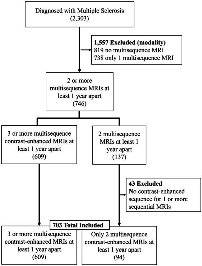
Flow chart of cohort selection
Table 1.
Demographic data of study cohort. Numbers are separated by those with 3 or more sequential MRIs of the cervical spine and those with only 2 MRIs (designated ). This distinction is important for further classification tasks in Experiment #3, below
| Sex | |
|---|---|
| Female | 464 + 73 (77%) |
| Male | 145 + 21 (23%) |
| Race | |
| White or Caucasian | 479 + 75 |
| - Hispanic or Latino | 38 + 5 |
| - Not Hispanic or Latino | 447 + 70 |
| Black or African American | 66 + 8 |
| Hispanic Caribbean | 10 + 2 |
| Asian | 4 + 1 |
| Arab of Middle Eastern | 4 + 1 |
| Multiracial | 1 |
| Other | 33 + 4 |
| Unable to determine/patient declined | 10 + 2 |
Data
Data Preprocessing
Original DICOMs are transformed into NIfTI files using MATLAB 2023b. Select sequences of T2-weighted, T1-weighted, and T1-weighted plus gadolinium contrast are selected and uploaded into a preprocessing Jupyter notebook. Spinal Cord Toolbox (https://spinalcordtoolbox.com/index.html) was used to find the centerline of the 3D NIfTI, and a straightened cord is produced. The resultant T2w straightened.nii is used to segment out the cord, and the resultant mask is used to subtract the surrounding tissues and vertebrae. Images are stacked as 3-channel (T1, T2, T1 +) and then concatenated into a "video"-type format with each frame representing a year of the patient’s MRI. Based upon a histogram of the total number of MRIs from the cohort, six (6) frames were selected as this was the median. For patients with less than 6 frames, the difference was divided by 6 and spaced accordingly (i.e., a patient with three scans in the years 2017, 2018, and 2023 would have them spaced in the following frame order: 2017, 2018, 2018, 2018, 2018, 2023). An example is demonstrated in Fig. 2.
Fig. 2.

Schematic of cord segmentation and preprocessing to a sequential, multichannel input as a six-frame "video." Initial processing of DICOM images to NIfTI utilizing MATLAB® with subsequent straightening using Spinal Cord Toolbox (https://github.com/spinalcordtoolbox/spinalcordtoolbox) results in a three-channel image containing the T1-weighted, T1 + contrast, and T2-weighted image (top). This is implemented for each year’s MRI for the patient and placed in sequential order (bottom)
Data Partitioning
Given the inherent class imbalance in EDSS, we utilized ADASYN (adaptive synthetic) sampling of the minority classes prior to normalization. To provide the models with full exposure to the data cohort, Stratified k-fold (k = 5) cross validation was implemented based upon prior works with large data imbalances [25]. Class-specific precision, recall, and harmonic mean are subsequently reported.
To our knowledge and efforts, we have not found an existing external validation set to evaluate the generalization of the model. To provide as much useful information as possible, we have provided a broad analysis of model architectures with an 20% hold-out testing split for all experiments prior to cross-validation on the remaining 80% of the data. The hold-out internal testing cohort was selected based upon temporal occurrence using the TRIPOD-AI guidelines [26].
Model Selection and Architectures
Model Selection and Optimization
We took inspiration from industry use of time-dependent deep learning models as seen in finance and meteorology. The time-dependency of the data necessitates the use of RNN models to provide temporal relationships between feature spaces in each patient, and to extract these feature spaces, we used traditional CNN-based architectures, resulting in a CNN-RNN model farm. These were used as a benchmark to test the more novel transformer models which provide encoding of each year (or frame) of patients’ images, giving the progression a form of “syntax” as seen in large language models (LLMs) in natural language processing (NLP) implementation. Finally, we created a competitive analysis based upon the trinary classification of EDSS using the entire dataset with further analysis of the best model from the convolutional and transformer-based architectures (Fig. 3). We used Keras Tuner (https://keras.io/keras_tuner/) Hyperband for initial hyperparameter tuning and optimization for learning rate, batch size, and dense layer size. Fine tuning was completed manually for the individual experiments.
Fig. 3.

Competitive analysis of convolutional-based architectures versus transformer-based models. Across five repeated random samplings (RRS), VGG16-LSTM and ViViT consistently had the highest validation and hold-out testing AUC on the entire dataset
CNN-RNN Architectures
Initial benchmarking for our time-dependent analysis was implemented using hybrid CNN-RNN models to address multivariate spatial and temporal data, respectively. Our initial competitive performance analysis included the use of pretrained ResNet50 and VGG16 architectures which were subsequently fed into LSTM. This architecture allowed for a temporal memory with limited gradient decay of the spatial data between each patient’s scans. A 3D representation of the individual multisequence MRI containing T1w, T1w + contrast, and T2w images into a three-channel image is represented as ((HxW)) with output volume as where F is kernel size, P is padding, and S is stride of the filter, and W is the input volume. The output feature map as . The resultant receptive field is calculated as follows: where is the filter size at layer , the stride of layer .
From each frame, these features are passed to the LSTM through an input gate:
where is the sigmoid function, , is the input gate, is the forget gate, is the output gate, x_t is the current input feature, and are the bias and weight for each gate neuron (respectively), is the output from the previous LSTM. For our experiment, a dropout of 0.5 was implemented.
ViT-based Architectures
An initial ViT architecture was used to patchify each multichannel image to provide tokenization for each frame. The input image is transformed into a flat feature vector of shape
where represents patches N∈{1:n} and E is the embedding projection. For each individual frame (year n multisequence MRI), the patches are flattened and multiplied by a trainable embedding tensor of dimension 1024. Each of the tokens is associated with sequential patch embeddings and fed into an LSTM for each frame prior to a linear classifier layer.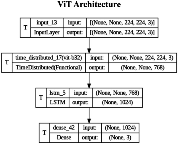
In contrast, the ViViT is a pure transformer architecture. Similar to ViT, patch embedding is prepended to a tokenized sequence resulting in a positional embedding, . These tokens are then passed to an encoder consisting of transformer layers, each with multi-headed attention (MHA) layers. Subsequently, this is passed to layer normalization (LN) and sequential dense layers of size 4d and 1d (d is number of classes) with Generalized Linear Rectifying Unit (GeLU) normalization at each layer.
The unique component of ViViT is Tubelet encoding that creates three-dimensional tokenized patches, , , , which are the temporal, height, and width dimensions, respectively. For our experiment, we tokenized the temporal dimension by size of two frames with spatial size of 56 × 56.
Evaluation Metrics
Evaluation of the experimental models as well as implementation details comparator SOTA was based upon their individual ROC-AUC favored over accuracy given the class imbalance, as shown in Eq. 5.
where is signal, is noise, is the sum of examples demonstrating the positive class label, is the negative class label, and is a designated cutoff (typically 0.5). To compare model variance and establish statistical significance of performance differences, a 5 × 2 cross-validation F-statistic is described by Alpaydin et al. [25], as shown in Eqs. 6–10. Internal model variance between training folds was measured using the 5 × 2 cross-validation T-statistic, as shown in Eq. 11.
| 1 |
| 2 |
| 3 |
| 4 |
| 5 |
| 6 |
| 7 |
| 8 |
| 9 |
| 10 |
| 11 |
Model Implementation
All models and experiments were implemented using TensorFlow Keras. The GPU is a single NVIDIA A100 with 80 GB GPU RAM. For data partitioning, the full dataset underwent random split of 20% for hold-out testing which was repeated with each RRS to avoid a biased set evaluation. This was implemented for all models at the onset of the competitive analysis (Fig. 1). In a separate experiment, the patients with only two sets of images (greater than or equal to 1 year apart) served as a hold-out testing set. The remaining data consisted of 3 or more years of imaging and underwent Stratified k-fold (k = 5) cross validation. Time to train (fine-tune for pretrained models) was measured for all models which assisted in which models would undergo final ablation analysis and clinical 2-channel evaluation.
Experimental Design
Experiment #1 is a competitive analysis of convolutional-based models (CNN-LSTM and CNN-GRU) seeded against one another with ROC-AUC as the measured metric, as well as a competitive analysis of transformer-based architectures (ViT-LSTM and ViViT) with similar measure. The best performing model from each category will proceed to Experiments #2 and #3.
Experiment #2 is an analysis of the impact of the individual timepoints on model performance. Sequential MRIs (frames) are incrementally removed from each patient’s collection of imaging, and subsequent ROC-AUC is compared against the CNN-RNN and transformer-based models selected from Experiment #1. These are then benchmarked against performance with all frames available.
Experiment #3 is an analysis of the impact of only two frames of data in comparison to patients who had 3 or more years of imaging. The select cohort of patients with only 2 scans serves as a separate hold-out testing set, and analysis of ROC-AUC is compared between the models selected from Experiment #1.
Experiment #4 is a study of the models’ ability to predict the exact EDSS value based upon the 11-point scale.
Interpretability
In an effort to better understand which imaging features of the individual frames were important to the model, a GradCAM may be used; however, we wanted to incorporate the four-dimensional weight and bias distribution throughout the ablation studies. For this, we utilized a multi-dimensional ablation analysis which sequentially passed a 3D patch (2D + time) of zeros across multiple frames at once and subsequently calculated the difference in output logits as described by Faghani et al. [27]. Examples of the resultant occlusion maps with instances of mislabeling and probabilities are shown for each experiment (Fig. 4).
Fig. 4.

Examples of misclassification with occlusion maps and classification probability
Results
Experiment #1: Competitive Model Analysis
Two families of time-dependent machine learning models underwent internal competitive analysis on the full dataset with the best performing model continuing to the next “round” in a bracket-based “playoff” scenario. In the CNN-RNN architecture branch, the LSTM-based models consistently outperformed their GRU counterparts. For the transformer-based branch, ViViT demonstrated the best performance consistently over the ViT-LSTM architecture with less memory requirements (Table 2).
Table 2.
Competitive performance analysis of the time-dependent models
| Model | Param (M) | Flops (G) | Internal Validation AUC (95% CI) | Hold-out Testing AUC |
|---|---|---|---|---|
| ResNet50-LSTM | 128 | 4.5 | 0.78 (0.75–0.81) | 0.76 |
| ResNet50-GRU | 31 | 4.3 | 0.74 (0.75–0.80) | 0.75 |
| VGG16-LSTM | 89 | 15.9 | 0.81 (0.70–0.87) | 0.85 |
| VGG16-GRU | 21 | 15.4 | 0.76 (0.71–0.86) | 0.74 |
| ViTL32-LSTM | 314 | 15.4 | 0.77 (0.68–0.78) | 0.70 |
| ViTB32-LSTM | 1170 | 15.1 | 0.78 (0.67–0.89) | 0.78 |
| ViViT | 838 | 4.9 | 0.83(0.81–0.86) | 0.84 |
Experiment #2: Data Ablation Study
Incremental subtraction of video frames (sequential MRIs) was performed to evaluate where each of the architectures began to experience performance loss. For each RRS, ROC-AUC and loss were measured after the introduction of only the first two, three, four, or five frames which were compared to the inclusion of all six frames (Table 3). A hold-out test set of 71 was constant for each stratified 5-fold split of training and validation data with a seed value of 42.
Table 3.
Ablation study of the time-dependency of deep learning models. P-values were calculated using paired Student's T-test for variance of mean between VGG-LSTM and ViViT Validation AUC
| Model | Frames 1–2 | Frames 1–3 | Frames 1–4 | Frames 1–5 | All Frames | |||||
|---|---|---|---|---|---|---|---|---|---|---|
| Val AUC (95% CI) | Test AUC | Val AUC (95% CI) | Test AUC | Val AUC (95% CI) | Test AUC | Val AUC (95% CI) | Test AUC | Val AUC (95% CI) | Test AUC | |
| VGG-LSTM | 0.75 (0.65–0.85) | 0.85 | 0.76 (0.68–0.84) | 0.80 | 0.75 (0.68–0.83) | 0.80 | 0.76 (0.71–0.81) | 0.80 | 0.74 (0.70–0.78) | 0.78 |
| ViViT | 0.80 (0.74–0.85) | 0.82 | 0.81 (0.77–0.86) | 0.79 | 0.81 (0.75–0.87) | 0.75 | 0.82 (0.77–0.85) | 0.77 | 0.81 (0.80–0.82) | 0.82 |
| p-value | 0.122 | 0.109 | 0.346 | 0.409 | 0.039 | |||||
Experiment #3: Temporal Depth Study
Given the difference in data density between those patients with six MRIs and those with only two, we performed an additional ablation study with removal of all patients with only two MRIs for training and validation, using this cohort as a hold-out test set (n = 94) (Fig. 5). A traditional 10% internal hold-out testing set was implemented for performance loss comparison (Table 4). While the VGG16-based architecture had a greater performance on the hold-out sparse cohort, the difference between the models was not statistically significant (p-value 0.361, 5 × 2 cross-validation F-test) (Fig. 6) (Table 5) [28].
Fig. 5.

Confusion matrices for trinary classification of hold-out testing on patients with only 2 sequential MRIs
Table 4.
Ablation study with two-scan cohort hold-out testing. P-value is calculated using paired Student's T-test for variance in mean between holdout testing AUC
| Model | Internal validation (3 + frames) AUC (95% CI) | Internal testing (3 + frames) AUC | Hold-out testing accuracy | Hold-out Ttesting AUC | ||
|---|---|---|---|---|---|---|
| VGG16-LSTM | 0.78 (0.70–0.87) | 0.81 | 0.57 | 0.75 | ||
| ViViT | 0.83 (0.78–0.89) | 0.84 | 0.61 | 0.72 | ||
| p-value | 0.361 | |||||
Fig. 6.


Occlusion maps for trinary EDSS prediction between models. A small patch of zeros is passed across the data and logit change is measured. Brighter pixels equate to more important features to the models. Predicted and Truth class labels are provided for each example. VGG = VGG16-LSTM, SVIT = ViViT. 0 = mild, 1 = moderate, 2 = severe disability
Table 5.
Class-based performance metrics
| Model | Class | Precision | Recall | F1-score |
|---|---|---|---|---|
| VGG16-LSTM | Mild | 0.69 | 0.66 | 0.68 |
| Moderate | 0.38 | 0.43 | 0.40 | |
| Severe | 0.58 | 0.47 | 0.52 | |
| ViViT | Mild | 0.68 | 0.81 | 0.74 |
| Moderate | 0.56 | 0.24 | 0.33 | |
| Severe | 0.39 | 0.60 | 0.47 |
Experiment #4: Exact EDSS Prediction Study
To further test the classification by the model, we analyzed the ability of the VGG16-LSTM and ViViT to pinpoint the individual EDSS scores for each patient demonstrating limited performance. As discussed above, there was a more considerable class imbalance and imbalance with this data set (Figs. 7 and 8).
Fig. 7.

Confusion matrices for hold-out testing on exact EDSS predictions (scale 0–10) for a Classification and b Regression architectures for the VGG16-LSTM (left) and ViViT (right)
Fig. 8.


Occlusion maps for exact EDSS prediction between models in classification. A small patch of zeros is passed across the data and logit change is measured. Brighter pixels equate to more important features to the models. Predicted and Truth class labels are provided for each example. VGG = VGG16-LSTM, SVIT = ViViT
Discussion
In this study, we demonstrate that time-dependent models can predict disability in MS using the EDSS as a predictive target outcome of trinary disability stratification. This mimics the categorization of disability seen in clinical practice where “mild” refers to no need for assistive devices, “moderate” refers to the use of sporadic cane up to bilateral support, and “severe” ranges from wheelchair-bound to death. Specifically, we found that both the CNN-RNN architecture and the ViViT had similar performance in this experiment, predicting EDSS with an AUC of 0.84 utilizing the whole dataset.
Additionally in experiment 3, we were able to demonstrate that the convolutional-based and transformer-based models both lost hold-out testing predictability performance when only presented with two studies when they have been trained on three or more. While patients may have undergone only a few scans at clinical presentation, this should be incorporated into the training data to anticipate this possibility and maintain predictive performance.
When we attempted to provide exact EDSS predication in experiment 4, the models did not perform as well. In exact EDSS classification, a performance of 0.77 AUC with a diminished F1-score was the best by ViViT but much lower than trinary classification.
We analyzed our results against the current literature. The majority of deep learning studies that investigated MS analyzed brain lesions, often with segmentation. For those studies implementing EDSS as a ground-truth label, the longest span was weeks to a few years. Additionally, fewer studies used multisequence MRI with gadolinium enhancement which indicates active demyelination. A variety of models were used in these studies; however, no study implemented either CNN-RNN or ViT-based architectures in their analysis (Table 6).
Table 6.
Exact EDSS prediction using both classification and regression
| Model | Internal validation AUC (95% CI) | Hold-out testing Acc | Hold-out testing AUC | Precision | Recall | F1-score (weighted mean) |
|---|---|---|---|---|---|---|
| VGG16-LSTM Classification | 0.75 (0.70–0.77) | 0.32 | 0.76 | 0.37 | 0.34 | 0.34 |
| VGG16-LSTM Regression | 0.74 (0.69–0.78) | 0.28 | 0.73 | 0.37 | 0.31 | 0.32 |
| ViViT Classification | 0.77 (0.71–0.79) | 0.30 | 0.77 | 0.37 | 0.34 | 0.33 |
| ViViT Regression | 0.70 (0.65–0.73) | 0.26 | 0.73 | 0.37 | 0.30 | 0.32 |
There has been a large number of studies which have investigated the classification of MS as well as its progression; however, the majority of studies which attempted to predict disability using the EDSS were often limited to small timeframes with the largest study spanning 5 years [29–35]. Studies that utilized imaging data (primarily MRI) for the prediction of EDSS analyzed brain lesions only, all of which were segmented. Only a small number of these studies utilized additional contrast-enhanced T1-weighted (T1w + contrast) sequences which would indicate active demyelination. While there were studies that implemented logistic regression techniques, the majority of recent literature utilized deep learning models (Table 7).
Table 7.
Comparison of prior studies. These studies reported modest performance with many utilizing prior SOTA techniques such as 3D CNNs and various SVM (support vector machine) or DTC (decision tree classifier) architectures. None of the existing studies reported the use of time-dependent architectures such as recurrent neural networks (RNNs) much less transformer architectures, which is necessary to account for changes over time and how they impact the prediction; however, there is a zeitgeist establishing the need for deep learning in the role of MS [29–35]
| Study | Location | EDSS | MRI sequences | Data | Model(s) | Patients | Metric |
|---|---|---|---|---|---|---|---|
| Our Study (Exp. #2) | US | Trinary (2–12 years) |
T1w T2w T1w + C |
Spinal cord (no lesion segmentation) |
VGG16-LSTM ViViT |
703 | 0.84 AUC |
| Our Study (Exp. #4) | US | Exact EDSS (2–12 years) |
T1w T2w T1w + C |
Spinal cord (no lesion segmentation) |
VGG16-LSTM ViViT |
703 | 0.77 AUC |
| Coll et al. (2023) [29] | Spain | Binary (< or > = 3) |
T1w T2w |
Brain lesions | 3D CNN Linear Regression | 319 | 0.79 Acc |
| Plati et al. (2022) [30] | Greece | Trinary (1-year change) | Not specified | Brain lesions + clinical data using ProMiSi software |
DTC ROT Naïve Bayes KNN SVM |
79 (50 low, 18 mod, 10 severe) | 0.83 Acc |
| Talon et al. (2022) [31] | Italy | Increase by > = 1.5, 1.0, 0.5 | T1w | Brain lesions | ResNet50 | 181 | 0.81 AUC |
| Pontillo et al. (2021) [32] | Italy | Exact prediction (mean EDSS 2.5) |
T1w T2w |
Brain lesion volume + radiomics |
Ridge Gaussian SVM RFR |
604 | 0.79 Acc |
| Tommasin et al. (2021) [33] | Italy | Binary | T2w | Brain lesion load + FA | RFC | 163 | 0.81 AUC |
| Tousignant et al. (2019) [34] | Canada | Increase by > = 1.5 (12 weeks) |
T1w + C T2w |
Brain lesions | 3D InceptionNet | 465 | 0.70 AUC |
| Zhao et al. (2017) [35] | US | Increase by > = 1.5 (1–5 years) | T2w | Brain lesion volumes | tenfold SVM | 1693 | 0.67 Acc |
Limitations of the study include the use of single institution data which may provide inherent bias and must be tested with external validation. As this dataset does not exist currently, we are in negotiations with other institutions to evaluate the models’ generalizability using federated learning.
Given the initial results, clinical implementation of the algorithm in neurology clinics is feasible given model and weight sharing; however, containerization and improved preprocessing must be completed beforehand. To further investigate this, future studies beyond external validation include prospective observational studies where patients presenting early in their disease course will have their initial imaging analyzed by the models to predict an EDSS within 3–6 years. The scores would be double-blinded as not to influence neuroimmunology upon scoring the patient, nor the patient to bias disability questionnaire responses. No treatment modification would be implemented at this time, and final prediction AUC would be tested against their ground truth.
Conclusion
In this study, we analyzed the ability of different time-dependent deep learning models to predict physical disability from MS based upon their EDSS. We demonstrated the improved classification accuracy of ViViT over pretrained CNN-LSTM models on the entire dataset following a competitive performance analysis of different architectures.
Our subsequent ablation study showed that the more spatial-dependent CNN-LSTM architecture demonstrated mildly improved performance on the hold-out testing set than the spatiotemporal transformer model, ViViT; however, the difference was not statistically significant. This is important clinically as patients with MS who present early in their clinical course may only have a few MRIs available for analysis versus those in the study with 6–12 years’ worth of data. Earlier prediction of disability may provide the selection of “high-risk” patients for earlier, more potent medical management. Additionally, these patients may be able to have a greater understanding of their prognosis so that they may better plan their lives, given the disease occurs during formative years.
The greatest potential impact of this study is for the patient. We attempt to provide a pilot methodology to provide these patients and their families with an opportunity to have greater informed decision making in possible more potent therapies earlier in their disease course, as well as planning to optimize quality of life.
Our proposed methodology for providing accurate prediction of disease progression may be extrapolated to other disease states where sequential imaging data is available. This ranges from short-term sequential imaging such as dynamic contrast-enhanced MRI (DCE-MRI) and multiphase CT and MRI as seen in hepatocellular or adrenal cancer, as well as long-term sequential imaging such as traumatic brain injury (TBI), Alzheimer’s disease (AD), and lung cancer following chemoradiation, for example.
Author Contributions
John Mayfield – Data scientist, engineer, primary author, first draft creation, IRB approval. Ryan Murtagh – Clinical radiology correlation and imaging reviewer, commented on manuscript revisions. John Ciotti – Patient identification, clinical neurology correlation, contributing author, IRB approval, contributing author, commented on manuscript revisions. Derrick Robertson – Patient identification, clinical neurology correlation, contributing author, IRB approval, contributing author, commented on manuscript revisions. Issam El Naqa – Data scientist, engineer, overall study design supervision, IRB approval, commented on manuscript revisions.
Data Availability
Models and weights are available upon request from the authors. Dataset is not currently available, however, the authors are currently negotiating a shareable repository with other institutions.
Declarations
Ethics Approval
This study was retrospective and did not involve change to treatment plans, additional radiation doses through increased diagnostic examinations, or release of patient information. The USF IRB committee approved a waiver and confirmed no ethical approval would be required.
Consent to Participate
Informed consent was waived per IRB as this was a retrospective study. Patients upon receiving any scan within the facility network sign a form stating their deidentified exams may be used for future research and teaching purposes.
Consent for Publication
The authors affirm that informed consent was waived per the IRB for publication of the images in Fig. 4.
Competing Interests
The authors declare no competing interests.
Footnotes
Previous presentation: Presentation of the abstract took place at 2023 ASFNR in Boston, MA.
Publisher's Note
Springer Nature remains neutral with regard to jurisdictional claims in published maps and institutional affiliations.
References
- 1.Rovira, Àlex, and Cristina Auger. “Beyond McDonald: updated perspectives on MRI diagnosis of multiple sclerosis.” Expert Review of Neurotherapeutics 21.8 (2021): 895–911. [DOI] [PubMed] [Google Scholar]
- 2.Wallin MT, Culpepper WJ, Campbell JD, Nelson LM, Langer-Gould A, Marrie RA, et al. The prevalence of MS in the United States. Neurology. 2019 Mar 5; 92(10): e1029–e1040. [DOI] [PMC free article] [PubMed] [Google Scholar]
- 3.Csepany, Tunde. “Diagnosis of multiple sclerosis: A review of the 2017 revisions of the McDonald criteria.” Ideggyogyaszati szemle 71.9–10 (2018): 321–329. [DOI] [PubMed] [Google Scholar]
- 4.Smyrke N, Dunn N, Murley C, Mason D. Standardized mortality ratios in multiple sclerosis: Systematic review with meta‐analysis. Acta Neurologica Scandinavica. 2022 Mar;145(3):360-70. [DOI] [PubMed] [Google Scholar]
- 5.Lycklama, Geert, et al. “Spinal-cord MRI in multiple sclerosis.” The Lancet Neurology 2.9 (2003): 555–562. [DOI] [PubMed] [Google Scholar]
- 6.McGinley, M.P., Goldschmidt, C.H. and Rae-Grant, A.D., 2021. Diagnosis and treatment of multiple sclerosis: a review. JAMA, 325(8), pp.765-779. [DOI] [PubMed] [Google Scholar]
- 7.Aslam, Nida, et al. “Multiple Sclerosis Diagnosis Using Machine Learning and Deep Learning: Challenges and Opportunities.” Sensors 22.20 (2022): 7856. [DOI] [PMC free article] [PubMed] [Google Scholar]
- 8.Afzal, HM Rehan, et al. “The emerging role of artificial intelligence in multiple sclerosis imaging.” Multiple Sclerosis Journal 28.6 (2022): 849–858. [DOI] [PubMed]
- 9.Seccia, Ruggiero, et al. “Machine learning use for prognostic purposes in multiple sclerosis.” Life 11.2 (2021): 122. [DOI] [PMC free article] [PubMed] [Google Scholar]
- 10.Eshaghi, Arman, et al. “Identifying multiple sclerosis subtypes using unsupervised machine learning and MRI data.” Nature communications 12.1 (2021): 1–12. [DOI] [PMC free article] [PubMed] [Google Scholar]
- 11.Shoeibi, Afshin, et al. “Applications of deep learning techniques for automated multiple sclerosis detection using magnetic resonance imaging: A review.” Computers in Biology and Medicine 136 (2021): 104697. [DOI] [PubMed] [Google Scholar]
- 12.Lukas C, Knol DL, Sombekke MH, Bellenberg B, Hahn HK, Popescu V, Weier K, Radue EW, Gass A, Kappos L, Naegelin Y. Cervical spinal cord volume loss is related to clinical disability progression in multiple sclerosis. Journal of Neurology, Neurosurgery & Psychiatry. 2015 Apr 1;86(4):410-8. [DOI] [PubMed] [Google Scholar]
- 13.Losseff NA, Webb SL, O'riordan JI, Page R, Wang L, Barker GJ, Tofts PS, McDonald WI, Miller DH, Thompson AJ. Spinal cord atrophy and disability in multiple sclerosis: a new reproducible and sensitive MRI method with potential to monitor disease progression. Brain. 1996 Jun 1;119(3):701-8. [DOI] [PubMed] [Google Scholar]
- 14.Cohen AB, Neema M, Arora A, Dell’Oglio E, Benedict RH, Tauhid S, Goldberg‐Zimring D, Chavarro‐Nieto C, Ceccarelli A, Klein JP, Stankiewicz JM. The relationships among MRI‐defined spinal cord involvement, brain involvement, and disability in multiple sclerosis. Journal of Neuroimaging. 2012 Apr;22(2):122-8. [DOI] [PMC free article] [PubMed] [Google Scholar]
- 15.Hidalgo de la Cruz M, Valsasina P, Meani A, Gallo A, Gobbi C, Bisecco A, Tedeschi G, Zecca C, Rocca MA, Filippi M. Differential association of cortical, subcortical and spinal cord damage with multiple sclerosis disability milestones: a multiparametric MRI study. Multiple Sclerosis Journal. 2022 Mar;28(3):406–17. [DOI] [PubMed]
- 16.Pravatà E, Valsasina P, Gobbi C, Zecca C, Riccitelli GC, Filippi M, Rocca MA. Influence of CNS T2-focal lesions on cervical cord atrophy and disability in multiple sclerosis. Multiple Sclerosis Journal. 2020 Oct;26(11):1402-9. [DOI] [PubMed] [Google Scholar]
- 17.Lee LE, Vavasour IM, Dvorak A, Liu H, Abel S, Johnson P, Ristow S, Au S, Laule C, Tam R, Li DK. Cervical cord myelin abnormality is associated with clinical disability in multiple sclerosis. Multiple Sclerosis Journal. 2021 Dec;27(14):2191-8. [DOI] [PMC free article] [PubMed] [Google Scholar]
- 18.Hochreiter S, Schmidhuber J. Long short-term memory. Neural computation. 1997 Nov 15;9(8):1735-80. [DOI] [PubMed] [Google Scholar]
- 19.Cho, K., Van Merriënboer, B., Gulcehre, C., Bahdanau, D., Bougares, F., Schwenk, H. and Bengio, Y., 2014. Learning phrase representations using RNN encoder-decoder for statistical machine translation. arXiv preprint arXiv:1406.1078.
- 20.Vaswani, A., Shazeer, N., Parmar, N., Uszkoreit, J., Jones, L., Gomez, A.N., Kaiser, Ł. and Polosukhin, I., 2017. Attention is all you need. Advances in neural information processing systems, 30.
- 21.Dosovitskiy, A., Beyer, L., Kolesnikov, A., Weissenborn, D., Zhai, X., Unterthiner, T., Dehghani, M., Minderer, M., Heigold, G., Gelly, S. and Uszkoreit, J., 2020. An image is worth 16x16 words: Transformers for image recognition at scale. arXiv preprint arXiv:2010.11929.
- 22.Wang, Z., Bai, Y., Zhou, Y. and Xie, C., 2022. Can cnns be more robust than transformers?. arXiv preprint arXiv:2206.03452.
- 23.Raghu, M., Unterthiner, T., Kornblith, S., Zhang, C. and Dosovitskiy, A., 2021. Do vision transformers see like convolutional neural networks?. Advances in Neural Information Processing Systems, 34, pp.12116–12128. [Google Scholar]
- 24.Arnab, A., Dehghani, M., Heigold, G., Sun, C., Lučić, M. and Schmid, C., 2021. Vivit: A video vision transformer. In Proceedings of the IEEE/CVF international conference on computer vision (pp. 6836–6846).
- 25.Szeghalmy, S. and Fazekas, A., 2023. A Comparative Study of the Use of Stratified Cross-Validation and Distribution-Balanced Stratified Cross-Validation in Imbalanced Learning. Sensors, 23(4), p.2333. [DOI] [PMC free article] [PubMed] [Google Scholar]
- 26.Collins, G.S. and Moons, K.G., 2019. Reporting of artificial intelligence prediction models. The Lancet, 393(10181), pp.1577–1579. [DOI] [PubMed] [Google Scholar]
- 27.Faghani, S., Khosravi, B., Zhang, K., Moassefi, M., Jagtap, J.M., Nugen, F., Vahdati, S., Kuanar, S.P., Rassoulinejad-Mousavi, S.M., Singh, Y. and Vera Garcia, D.V., 2022. Mitigating bias in radiology machine learning: 3. Performance metrics. Radiology: Artificial Intelligence, 4(5), p.e220061. [DOI] [PMC free article] [PubMed] [Google Scholar]
- 28.Alpaydm E. Combined 5× 2 cv F test for comparing supervised classification learning algorithms. Neural computation. 1999 Nov 15;11(8):1885-92. [DOI] [PubMed] [Google Scholar]
- 29.Coll, L., Pareto, D., Carbonell-Mirabent, P., Cobo-Calvo, Á., Arrambide, G., Vidal-Jordana, Á., Comabella, M., Castilló, J., Rodríguez-Acevedo, B., Zabalza, A. and Galán, I., 2023. Deciphering multiple sclerosis disability with deep learning attention maps on clinical MRI. NeuroImage: Clinical, 38, p.103376. [DOI] [PMC free article] [PubMed] [Google Scholar]
- 30.Plati D, Tripoliti E, Zelilidou S, Vlachos K, Konitsiotis S, Fotiadis DI. Multiple Sclerosis Severity Estimation and Progression Prediction Based on Machine Learning Techniques. In2022 44th Annual International Conference of the IEEE Engineering in Medicine & Biology Society (EMBC) 2022 Jul 11 (pp. 1109–1112). IEEE. [DOI] [PubMed]
- 31.Taloni A, Farrelly FA, Pontillo G, Petsas N, Giannì C, Ruggieri S, Petracca M, Brunetti A, Pozzilli C, Pantano P, Tommasin S. Evaluation of Disability Progression in Multiple Sclerosis via Magnetic-Resonance-Based Deep Learning Techniques. International Journal of Molecular Sciences. 2022 Sep 13;23(18):10651. [DOI] [PMC free article] [PubMed] [Google Scholar]
- 32.Pontillo G, Tommasin S, Cuocolo R, Petracca M, Petsas N, Ugga L, Carotenuto A, Pozzilli C, Iodice R, Lanzillo R, Quarantelli M. A combined radiomics and machine learning approach to overcome the clinicoradiologic paradox in multiple sclerosis. American Journal of Neuroradiology. 2021 Nov 1;42(11):1927-33. [DOI] [PMC free article] [PubMed] [Google Scholar]
- 33.Tommasin S, Cocozza S, Taloni A, Giannì C, Petsas N, Pontillo G, Petracca M, Ruggieri S, De Giglio L, Pozzilli C, Brunetti A. Machine learning classifier to identify clinical and radiological features relevant to disability progression in multiple sclerosis. Journal of Neurology. 2021 Dec;268(12):4834-45. [DOI] [PMC free article] [PubMed] [Google Scholar]
- 34.Roca P, Attye A, Colas L, Tucholka A, Rubini P, Cackowski S, Ding J, Budzik JF, Renard F, Doyle S, Barbier EL. Artificial intelligence to predict clinical disability in patients with multiple sclerosis using FLAIR MRI. Diagnostic and Interventional Imaging. 2020 Dec 1;101(12):795–802. [DOI] [PubMed] [Google Scholar]
- 35.Zhao Y, Healy BC, Rotstein D, Guttmann CR, Bakshi R, Weiner HL, Brodley CE, Chitnis T. Exploration of machine learning techniques in predicting multiple sclerosis disease course. PloS one. 2017 Apr 5;12(4):e0174866. [DOI] [PMC free article] [PubMed] [Google Scholar]
Associated Data
This section collects any data citations, data availability statements, or supplementary materials included in this article.
Data Availability Statement
Models and weights are available upon request from the authors. Dataset is not currently available, however, the authors are currently negotiating a shareable repository with other institutions.