Abstract
GM(1,1) model is widely used because it does not require a large number of samples and has a low computational complexity and no limitation of statistical assumptions. Common drawback of the GM(1,1) models developed by various techniques for improving the performance is their unsatisfied predicting accuracy although they have satisfied fitting accuracy. The aim of this paper is to develop GM(1,1) model with excellent predicting accuracy rather than fitting one. We proposed an improved GM(1,1) model based on weighted mean squared error (MSE) and optimal weighted background value: OB-WMSE-GM(1,1). To illustrate its effectiveness, it was applied to one simulation example and two application examples. For the exponential function simulation example, the fitting MSE, fitting WMSE and predicting MSE of the proposed GM(1,1) (0.000002, 0.000039 and 0.015485) were much lower than ones of the typical GM(1,1) (0.001492, 0.002606 and 1.144524). For the annual LCD TV output prediction example, the fitting MSE, fitting WMSE and predicting MSE of the proposed GM(1,1) (1.425255, 3.199446 and 132.046775) were much lower than ones of the typical GM (1,1) (48.003290, 111.431942 and 5519.135753). For the crude oil processing volume prediction example, the fitting MAPE, fitting WMRE and predicting MAPE of the proposed GM(1,1) (4.090405, 3.213106 and 3.775669) were lower than ones of the typical GM(1,1) (4.399448, 3.883765 and 5.040509). When the proposed method is properly combined with the other various techniques including metabolic mechanism, residual GM(1,1), original sequence pre-processing, background value reconstruction and initial condition optimization, its performance may be more and more improved.
Keywords: GM(1,1); Weighted mean squared error (MSE); Weighted background value; Pipeline corrosion prediction
Subject terms: Chemical engineering, Electrical and electronic engineering, Information technology
Introduction
In general, there are different types of uncertain systems with small samples and poor information in real world. Grey system is a system with partially known (white) and partially unknown (black) information1–3. Grey model plays an important role for modelling, prediction, evaluation, decision making, control and system analysis in many fields because of its advantages of simple expression and computation, and excellent prediction performance with insufficient data4.
GM(1,1) model is an important part of grey model, where ‘GM’ indicates ‘Grey Model’, the first number ‘1’ in brackets indicates the first order differential equation, and the second number ‘1’ indicates the differential equation of one variable. It is based on first order linear ordinary differential equation and least square method, mathematically. It requires a relatively small amount of data (four or more samples) to develop a mathematical model, and a simple calculation process to analyse the behaviour of the unknown system. It has been widely used because it does not require a large number of samples and has a low computational complexity and no limitation of statistical assumptions1,5,6.
The GM(1,1) model is based on accumulated generating operation (AGO), which is the most crucial characteristic of the grey theory. The purpose of the AGO is smoothing the data and reducing the randomness in the raw data, and converting it to a monotonic increasing function5.
Up to now, many research works to improve the accuracy of the GM(1,1) have been performed on the following aspects: optimization of initial condition, reconstruction of background values, pre-processing of original sequence, error compensation with a residual GM(1,1) model, optimization of model internal parameters, improvement of time response function, combination model, and introducing of intelligent global optimization algorithms2,3,7–10.
To evaluate the accuracy of the GM(1,1) models, mean absolute error (MAE), mean absolute percentage error (MAPE), mean squared error (MSE), and root mean squared error (RMSE) are commonly used10,11. In fact, since the prediction or forecast can be said as a technique to predict the future values by paying attention and considering past and present data12, the predicting accuracy should be considered as the main performance for the prediction model rather than the fitting accuracy. Although the prediction model has high fitting accuracy, the model without high predicting accuracy is no reasonable to use in the practice. Therefore, it should be paid attention to improve the predicting accuracy rather than the fitting accuracy due to the original purpose of the prediction model. However, many previous methods for improving the accuracy of the grey models used the MAE, MAPE, MSE and RMSE as the accuracy measures of the developed models13–18. The accuracy measures were calculated using the arithmetic average operation of the errors at the fitting points, and they include no sufficient information about the predicting accuracy. Consequently, the almost previous works may be regarded as the works for improving the fitting accuracy of the GM(1,1). It may be a common drawback of the previous works for improving the performance of the GM(1,1). When we use the accuracy evaluating measures with more sufficient information about the predicting accuracy, it is possible to use for improving the predicting accuracy of the prediction model.
The higher the accuracy at the recent fitting points is, the higher the predicting accuracy at the predicting points may be. Therefore, the accuracy evaluating measure has to better reflect the accuracy of the recent fitting points near to the last fitting point of the original sequence than the accuracy of the past fitting points father to the last fitting point. To do this, we introduce weighted mean squared error (WMSE), where the weights of the recent fitting points near to the last fitting point have to be higher than the weights of the past fitting points farther to the last fitting point, and proposes a new improved GM(1,1) model based on WMSE and optimal weighted background value: OB-WMSE-GM(1,1).
The remaining parts of the paper are organized as follows. The following section describes the main steps to develop the typical GM(1,1) and improved GM(1,1) model based on WMSE and optimal background value: OB-WMSE-GM(1,1). The next section applies the proposed method to one simulation example and two application examples to illustrate its effectiveness.
Methods
Method to develop typical GM(1,1)
Let X(0) = {x(0)(1),…, x(0)(k),…, x(0)(n)} be an original non-negative sequence (n ≥ ←∆), where x(0)(k) represents the behavior of the data at the time index k.
The main steps to develop the typical GM(1,1) are as follows1–3,10,13:
Step 1. Construct the accumulated generating operation (AGO) sequence X(1) = {x(1)(1),…, x(1)(k),…, x(1)(n)} from the original sequence X(0) using the following equation:
 |
1 |
Step 2. Calculate the background value z(1)(k) of x(1)(k) using the following equation: ( )
)
 |
2 |
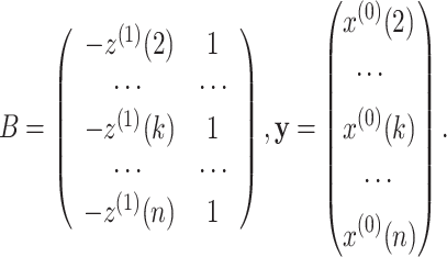
Step 3. Construct a matrix B and vector y as follows:
 |
3 |
Step 4. Calculate the vector  using the following equation:
 |
4 |
where  and
and  are the estimated values of development coefficient a and grey input u.
Step 5. Calculate the parameter C of the GM(1,1) using the following equation:
 |
5 |
Step 6. Develop the GM(1,1) as follows:
 |
6 |
It is the equation to calculate the time response sequence of the GM(1,1).
By substituting k = n + 1 into Eq. (6), we can predict the future value at k = n + 1. By substituting k = n + 2 into Eq. (6), we can predict the future value at k = n + 1. This procedure continues to the needed times.
To evaluate the accuracy performance of the developed GM (1, 1) model, we introduce the following evaluation measures:
(1) Absolute error (AE), and mean absolute error (MAE):
 |
7 |
 |
8 |
(2) Absolute percentage error (APE), and mean absolute percentage error (MAPE):
 |
9 |
 |
10 |
Method to develop an improved GM(1,1) based on weighted mean squared error and optimal weighted background value: OB-WMSE-GM(1,1)
As can be seen in the time response equation  of the GM(1,1), the parameter C is one of the influencing factors on the accuracy of the GM(1,1). In the typical GM(1,1), the value of the parameter C is calculated using Eq. (5).
As the major aim of the GM(1,1) is to predict the future values by considering and using the past and present data, it is desirable to improve the predicting accuracy of the GM(1,1) rather than the fitting accuracy.
The fitting errors at the last fitting points may has higher influence on the predicting error at the future predicting points, while the fitting errors at the front fitting points may has lower influence on the predicting error at the future predicting points. Therefore, we have to improve the fitting accuracy at the last points in the original data sequence rather than the front points to more and more improve the predicting accuracy for the future values.
To do this, we first introduce a weighted mean squared error (WMSE):
 |
11 |
by generalizing the typical mean squared error (MSE):
 |
12 |
where w(2),…, w(k),…, and w(n) are the importance weights of each point, and they have to satisfy w(2),…, w(k),…, w(n) ≥ 0, and  .
.
When w(2) = … = w(k) = … = w(n) = 1/(n-1), the WMSE in Eq. (11) becomes to the typical MSE in Eq. (12).
In this work, we try to find the best value of the parameter C to minimize the WMSE in Eq. (11).
We have
 |
13 |
Since the function WMSE(C) is a quadratic function with one extreme point, we can determine optimal C to minimize the function WMSE(C) by the extremum principle.
We have
 |
14 |
By the extremum principle, we have to solve the following equation:
 |
15 |
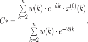
From Eq. (15), we have
 |
16 |
It becomes the best value of the parameter C to minimize the WMSE.
Consequently, the improved GM(1,1) based on the WMSE is as follows:
 |
17 |
As can be seen in Eq. (17), the key parameters are C* and  , and therefore the accuracy of the model depends on the parameters. The value of C* is calculated using Eq. (16), and the value of
  is calculated using Eq. (4). In Eq. (4), the matrix B contains the background values z(1)(k);
  . Consequently, the background values also affect the accuracy of the GM(1,1), and it is possible to more increase the accuracy of the GM(1,1) by using the reasonable background values.
To more improve the accuracy of the GM(1,1), this subsection intoduces the following weighted background values:
 |
18 |
where p is the background weight. In the typical GM(1,1), p is commonly equal to 0.5.
When the value of p is appropriately selected, the accuracy of the GM(1,1) may be more increased.
We determine the optimal background weight p so that the GM(1,1) has the minimum WMSE by varying the value of p between 0 and 1 with a fine spacing.
The main steps to develop an improved GM(1,1) based on WMSE and optimal weighted background value are as follows:
Step 1. Construct the accumulated generating operation (AGO) sequence X(1) = {x(1)(1),…, x(1)(k),…, x(1)(n)} from the original sequence X(0) using Eq. (1).
Step 2. Calculate the weights w(k) = 2(k-1)/[n(n-1)], k = 2, 3, …, n.
Step 3. p = 0, minWMSE = 1,000,000.
Step 4. Calculate the weighted background values z(1)(k);  using Eq. (18).
Step 5. Construct a matrix B and vector y using Eq. (3).
Step 6. Calculate the vector  using Eq. (4).
Step 7. Calculate the optimal value C* of the GM(1,1) with mininum WMSE using Eq. (16).
Step 8. Develop the GM(1,1) using Eq. (17).
Step 9. Evaluate the WMSE WMSE(p) of the GM(1,1).
Step 10. If WMSE(p) < minWMSE then minWMSE = WMSE(p) and p* = p.
Step 11. p = p + dp. If p ≤ 1 then go to Step 3. dp is a varied spacing for p. In this work, dp = 0.01.
Step 12. Determine p* as the optimal background weight, and select the corresponding GM(1,1) with optimal p* as the optimal GM(1,1).
The above-mentioned model is called improved GM(1,1) based on WMSE and optimal weighted background value, namely, OB-WMSE-GM(1,1).
In order that the weights of the recent fitting points have higher values than the past fitting points, this work determines the weights w(2),…, w(k),…, and w(n) as follows:
 |
19 |
where r is called weighting factor. It is sure that  .
.
If r = 1 then it indicates that the past data and recent data play the same roles to develop the GM(1,1), and if r > 1 then it indiates that the recent data play more important role than the past data. The predicting performance of the GM(1,1) may depend on selecting the weighting factor r. When the value of r is too higher, the information of the past some fitting points may be ignored.
For example, when n = 5 and r = 2.5, the importance weights are w(2) = 0.039, w(3) = 0.099, w(4) = 0.246, w(5) = 0.616. Since the importance weight of the last fitting point w(5) is 0.616, and the importance weights of the second and third fitting points w(2) and w(3) are respectively 0.039 and 0.099, the recent information is too emphasized and the past informations are almost ignored. The same can be said of r = 2.0. As the result, we can know that it is necessary to select the suitable value of r. According to the authors’ practical experience and the reference14, this work selected the value of weighting factor as r = 1.5.
Results and discussion
This section applied the proposed methods to two examples: two examples: exponential function simulation example and mine tailings pipeline corrosion prediction problem. The authors developed the MATLAB program for the proposed methods, and applied them to solve the examples.
Simulation example
As one simulation example, this subsection took the simulated data sequence obtained from the exponential function f(t) = e0.3t, t = 1, 2,…, 14. Namely, the simulated data sequence was as follows:
{1.349859, 1.822119, 2.459603, 3.320117, 4.481689, 6.049647, 8.166170, 11.023176, 14.879732, 20.085537, 27.112639, 36.598234, 49.402449, 66.686331}.
For the simulation example, we selected the exponential function f(t) = e0.3t because the GM(1,1) model with -a ≤ 0.3 is applicable to middle and long term prediction, where a is a development coefficient.
In the above simulated data sequence, the first five values X(0) = {1.349859, 1.822119, 2.459603, 3.320117, 4.481689} were used to develop the GM(1,1) and evaluate its fitting accuracy. The last eight values Xt = {6.049647, 8.166170, 11.023176, 14.879732, 20.085537, 27.112639, 36.598234, 49.402449, 66.686331} were used to evaluate the predicting accuracy of the GM(1,1).
We developed the typical GM(1,1) with the original data sequence X(0). The parameter values a and u were a = -0.297770, u = 1.148885, and the parameter value C was C = 0.995837. Consequently, the typical GM(1,1) was as follows:
 |
20 |
Next, we developed the OB-WMSE-GM(1,1) with weighting factor r = 1.5 using the proposed method.
The importance weights were respectively w(2) = 0.123077, w(3) = 0.184615, w(4) = 0.276923, w(5) = 0.415385, the optimal background weight p* was p* = 0.48, the parameter values a and u were a = -0.299554, u = 1.155768, and the optimal parameter value C* was C* = 1.002007. Consequently, the OB-WMSE-GM(1,1) was as follows:
 |
21 |
Table 1 shows the fitting (k = 1, 2,…, 5) and predicting (k = 6, 7,…, 14) accuracy test results of the typical GM(1,1) and proposed OB-WMSE-GM(1,1): Eqs. (20) and (21).
Table 1.
Fitting and predicting accuracy test results of typical and proposed GM(1,1) models: Eqs. (20) and (21).
| k | True value | Typical GM(1,1) | OB-WMSE-GM(1,1) | ||||
|---|---|---|---|---|---|---|---|
| Calculated value | AE | APE (%) | Calculated value | AE | APE (%) | ||
| 1 | 1.349859 | 1.349859 | 0.000000 | 0.000000 | 1.349859 | 0.000000 | 0.000000 |
| 2 | 1.822119 | 1.806459 | 0.015660 | 0.859415 | 1.824148 | 0.002029 | 0.111358 |
| 3 | 2.459603 | 2.433033 | 0.026570 | 1.080246 | 2.461244 | 0.001641 | 0.066721 |
| 4 | 3.320117 | 3.276936 | 0.043181 | 1.300585 | 3.320851 | 0.000734 | 0.022105 |
| 5 | 4.481689 | 4.413548 | 0.068141 | 1.520432 | 4.480681 | 0.001008 | 0.022492 |
| 6 | 6.049647 | 5.944396 | 0.105251 | 1.739791 | 6.045590 | 0.004057 | 0.067069 |
| 7 | 8.166170 | 8.006222 | 0.159948 | 1.958660 | 8.157054 | 0.009116 | 0.111626 |
| 8 | 11.023176 | 10.783197 | 0.239979 | 2.177042 | 11.005962 | 0.017214 | 0.156163 |
| 9 | 14.879732 | 14.523371 | 0.356360 | 2.394938 | 14.849871 | 0.029861 | 0.200680 |
| 10 | 20.085537 | 19.560833 | 0.524704 | 2.612348 | 20.036292 | 0.049245 | 0.245178 |
| 11 | 27.112639 | 26.345548 | 0.767091 | 2.829274 | 27.034106 | 0.078533 | 0.289655 |
| 12 | 36.598234 | 35.483556 | 1.114679 | 3.045717 | 36.475955 | 0.122279 | 0.334113 |
| 13 | 49.402449 | 47.791101 | 1.611349 | 3.261677 | 49.215436 | 0.187013 | 0.378551 |
| 14 | 66.686331 | 64.367543 | 2.318788 | 3.477157 | 66.404269 | 0.282062 | 0.422969 |
Table 2 shows the mean fitting and predicting accuracy test results of the typical GM(1,1) Eq. (20) and proposed OB-WMSE-GM(1,1) Eq. (21). In Table 3, the WMAE and WMAPE respectively indicate the weighted MAE and weighted MAPE as follows:
 |
22 |
 |
23 |
Table 2.
Mean fitting and predicting accuracy test results of typical and proposed GM(1,1) models: Eqs. (20) and (21).
| Mean fitting performance | Mean predicting performance | ||||||||
|---|---|---|---|---|---|---|---|---|---|
| MAE | MAPE | MSE | WMAE | WMAPE | WMSE | MAE | MAPE | MSE | |
| Typical GM(1,1) | 0.030710 | 0.952136 | 0.001492 | 0.047095 | 1.296930 | 0.002606 | 0.799794 | 2.610734 | 1.144524 |
| Proposed GM(1,1) | 0.001082 | 0.044535 | 0.000002 | 0.001175 | 0.041488 | 0.000039 | 0.086598 | 0.245112 | 0.015485 |
Table 3.
Fitting and predicting accuracy test results of typical and proposed GM(1,1) models: Eqs. (24) and (25).
| k | Year | True value | Typical GM(1,1) | OB-WMSE-GM(1,1) | ||||
|---|---|---|---|---|---|---|---|---|
| Calculated value | AE | APE (%) | Calculated value | AE | APE (%) | |||
| 1 | 1996 | 3.280000 | 3.280000 | 0.000000 | 0.000000 | 3.280000 | 0.000000 | 0.000000 |
| 2 | 1997 | 5.480000 | 4.819230 | 0.660770 | 12.057856 | 5.533047 | 0.053047 | 0.968017 |
| 3 | 1998 | 10.070000 | 8.370397 | 1.699603 | 16.877885 | 9.699805 | 0.370195 | 3.676215 |
| 4 | 1999 | 17.700000 | 14.538329 | 3.161671 | 17.862546 | 17.004413 | 0.695587 | 3.929873 |
| 5 | 2000 | 29.730000 | 25.251254 | 4.478746 | 15.064736 | 29.809882 | 0.079882 | 0.268691 |
| 6 | 2001 | 49.390000 | 43.858260 | 5.531740 | 11.200121 | 52.258733 | 2.868733 | 5.808328 |
| 7 | 2002 | 92.670000 | 76.176295 | 16.493705 | 17.798322 | 91.613084 | 1.056916 | 1.140516 |
| 8 | 2003 | 162.230000 | 132.308668 | 29.921332 | 18.443773 | 160.603914 | 1.626086 | 1.002333 |
| 9 | 2004 | 280.860000 | 229.803555 | 51.056445 | 18.178610 | 281.549493 | 0.689493 | 0.245493 |
| 10 | 2005 | 513.400000 | 399.139943 | 114.260057 | 22.255562 | 493.575249 | 19.824751 | 3.861463 |
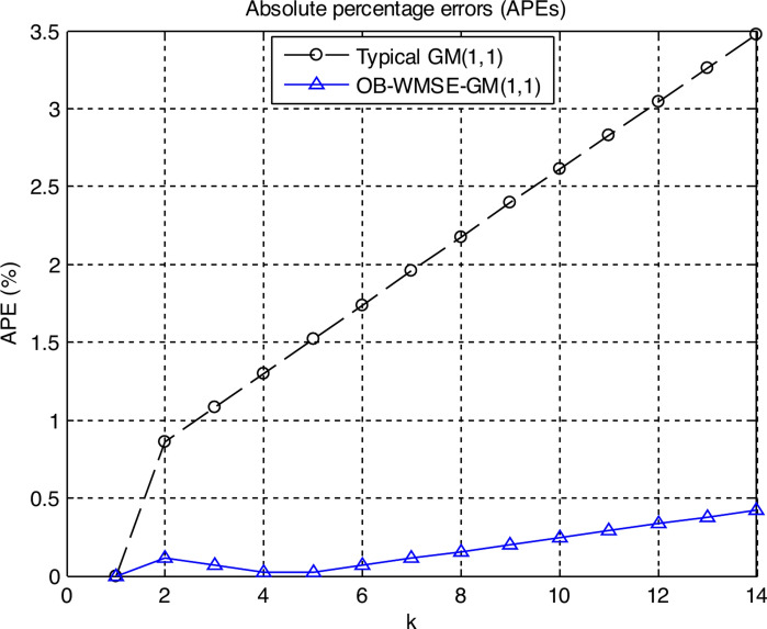
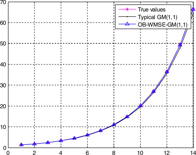
Figure 1 shows the graph of the APEs of the typical GM(1,1) and OB-WMSE-GM(1,1). In Fig. 1, the points from k = 1 to k = 5 indicate the fitting points, and the points from k = 6 to k = 14 indicate the predicting points. Figure 2 shows the graph of the true values, fitting and predicting values of the typical GM(1,1) and OB-WMSE-GM(1,1).
Fig. 1.
Graph of the APEs of the typical GM(1,1) and OB-WMSE-GM(1,1).
Fig. 2.
Graph of the true values, fitting and predicting values of the typical GM(1,1) and OB-WMSE-GM(1,1).
Tables 1–2 and Figs. 1–2 numerically and visually illustrated that the fitting and predicting accuracy of the proposed OB-WMSE-GM(1,1) were significantly much higher than the typical GM(1,1).
On the other hand, look at the APEs from the first fitting point (k = 1) to the last fitting point (k = 5) of the original sequence in Tables 1–2 and Figs. 1–2. The APEs of the proposed OB-WMSE-GM(1,1) were significantly trending downward from the second fitting point (k = 2) to the last fitting point (k = 5), while the APEs of the typical GM(1,1) were significantly trending upward. Namely, the closer the fitting point is to the last point (k = 5) of the original sequence, the lower the fitting errors of the proposed OB-WMSE-GM(1,1) become, while the higher the fitting error of the typical GM(1,1) becomes. It is because that we introduced the WMSE to improve the predicting accuracy of the GM(1,1).
The simulation result clearly demonstrated that the proposed OB-WMSE-GM(1,1) was pretty superior to the typical GM(1,1) from the viewpoints of not only fitting accuracy but also predicting accuracy.
Application examples
In the application examples, we selected the annual LCD TV output and crude oil processing volume prediction examples2,3 for demonstrating the details of the proposed method and comparing its performance with the performance of the typical GM(1,1) model and previous methods.
Case 1: Annual LCD TV output prediction
This subsection developed the GM(1,1) for predicting the annual LCD TV output of China.
The historical annual LCD TV output of China from 1996 to 2005 are as follows:2
3.28, 5.48, 10.07, 17.70, 29.73, 49.39, 92.67, 162.23, 280.86, 513.40.
The first seven values (from 1996 to 2002) X(0) = {3.28, 5.48, 10.07, 17.70, 29.73, 49.39, 92.67} were used to develop the OB-WMSE-GM(1,1) and evaluate its fitting accuracy. The last three values (from 2003 to 2005) Xt = {162.23, 280.86, 513.40} were used to evaluate the predicting accuracy of the OB-WMSE-GM(1,1).
We developed the typical GM(1,1) with the original data sequence X(0). The parameter values a and u were a = -0.552087, u = 1.799857, and the parameter value C was C = 1.597499. Consequently, the typical GM(1,1) was as follows:
 |
24 |
Next, we developed the OB-WMSE-GM(1,1) with weighting factor r = 1.5 using the proposed method.
The importance weights w(2), w(3),…, w(7) were respectively 0.048120, 0.072180, 0.108271, 0.162406, 0.243609, 0.365414, the optimal background weight p* was p* = 0.47, the parameter values a and u were a = -0.561367, u = 1.831217, and the optimal parameter value C* was C* = 1.800392. Consequently, the OB-WMSE-GM(1,1) was as follows:
 |
25 |
Table 3 shows the fitting (k = 1, 2,…, 7) and predicting (k = 8, 9, 10) accuracy test results of the typical and proposed GM(1,1) models: Eqs. (24) and (25). Table 4 shows the mean fitting and predicting accuracy test results of the typical GM(1,1) Eq. (24) and proposed OB-WMSE-GM(1,1) Eq. (25).
Table 4.
Mean fitting and predicting accuracy test results of the typical and proposed GM(1,1) models: Eqs. (24) and (25)
| Mean fitting performance | Mean predicting performance | ||||||||
|---|---|---|---|---|---|---|---|---|---|
| MAE | MAPE | MSE | WMAE | WMAPE | WMSE | MAE | MAPE | MSE | |
| Typical GM(1,1) | 4.575176 | 12.980209 | 48.003290 | 8.598771 | 15.411273 | 111.431941 | 65.079278 | 19.625982 | 5519.135753 |
| Proposed GM(1,1) | 0.732052 | 2.255949 | 1.425255 | 1.202619 | 2.612780 | 3.199446 | 7.380110 | 1.703097 | 132.046775 |
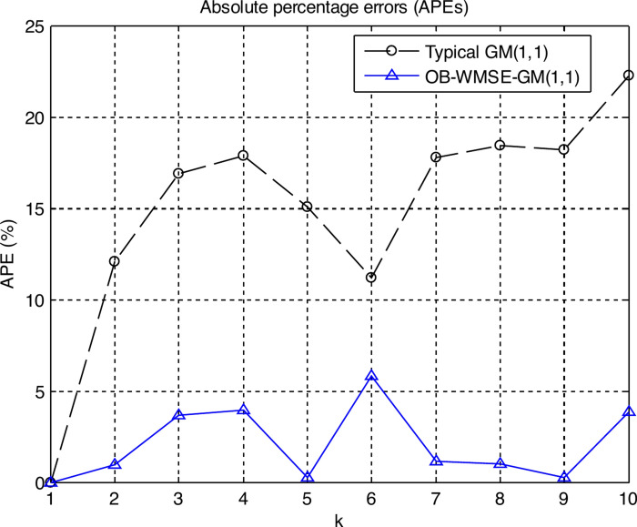
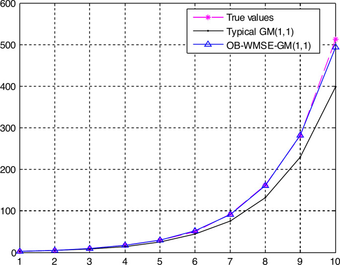
Figure 3 shows the graph of the APEs of the typical GM(1,1) and OB-WMSE-GM(1,1). In Fig. 3, the points from k = 1 to k = 7 indicate the fitting points, and the points from k = 8 to k = 10 indicate the predicting points. Figure 4 shows the graph of the true values, fitting and predicting values of the typical GM(1,1) and OB-WMSE-GM(1,1) models: Eqs. (24) and (25).
Fig. 3.
Graph of the APEs of the typical and proposed GM(1,1) models: Eqs. (24) and (25).
Fig. 4.
Graph of the true values, fitting and predicting values of the typical and proposed GM(1,1) models: Eqs. (24) and (25).
Tables 3–4 and Figs. 3–4 numerically and visually illustrated that the fitting and predicting accuracy of the proposed OB-WMSE-GM(1,1) were significantly much higher than the typical GM(1,1).
Finally, we compared the APEs and MAPEs at the fitting and predicting points of the proposed OB-WMSE-GM(1,1) with the ones of the previous similar work (improved GM(1,1) based on initial condition optimization) proposed by Madhi et al.2. As can be seen in Table 3, for the proposed OB-WMSE-GM(1,1), the APEs at the fitting points (k = 1, 2, …, 7) were respectively 0.000000, 0.968017, 3.676215, 3.929873, 0.268691, 5.808328, 1.140516, and the MAPE was 2.255949%. The APEs at the predicting points (k = 8, 9, 10) were respectively 1.002333, 0.245493, 3.861463, and the MAPE was 1.703097%. Meanwhile, for the previous GM(1,1) proposed by Madhi et al.2, the APEs at the fitting points were respectively 0.000000, 4.927007, 0.794439, 1.977401, 1.345442, 5.972869, 1.910003, and the MAPE was 2.821194%. The APEs at the predicting points were respectively 2.681378, 2.364167, 7.228282, and the MAPE was 4.091276%. By comparing the APEs and MAPEs, it is clear that the proposed OB-WMSE-GM(1,1) is pretty superior to the previous GM(1,1).
Case 2: Crude oil processing volume prediction
This subsection developed the GM(1,1) for predicting the crude oil processing volume.
The processing volumes from 1983 to 1994 are as follows:3
7490, 7665, 7904, 8565, 9718, 10,164, 10,528, 9783, 10,250, 10,815, 11,290, 11,000.
The first ten values (from 1983 to 1992) X(0) = {7490, 7665, 7904, 8565, 9718, 10,164, 10,528, 9783, 10,250, 10,815} were used to develop the OB-WMSE-GM(1,1) and evaluate its fitting accuracy. The last two values (from 1993 to 1994) Xt = {11,290, 11,000} were used to evaluate the predicting accuracy of the OB-WMSE-GM(1,1).
We developed the typical GM(1,1) with the original data sequence X(0). The parameter values a and u were a = -0.038969, u = 7631.408923, and the parameter value C was C = 7473.893931. Consequently, the typical GM(1,1) was as follows:
 |
26 |
Next, we developed the OB-WMSE-GM(1,1) with weighting factor r = 1.5 using the proposed method.
The importance weights w(2), w(3),…, w(10) were respectively 0.013354, 0.020030, 0.030045, 0.045068, 0.067602, 0.101403, 0.152105, 0.228157, 0.342236, the optimal background weight p* was p* = 1.0, the parameter values a and u were a = -0.038414, u = 7475.605881, and the optimal parameter value C* was C* = 7431.224183. Consequently, the OB-WMSE-GM(1,1) was as follows:
 |
27 |
Table 5 shows the fitting (k = 1, 2,…, 10) and predicting (k = 11, 12) accuracy test results of the typical and proposed GM(1,1): Eqs. (26) and (27).
Table 5.
Fitting and predicting accuracy test results of typical and proposed GM(1,1) models: Eqs. (26) and (27).
| k | Year | True value | Typical GM(1,1) | OB-WMSE-GM(1,1) | ||||
|---|---|---|---|---|---|---|---|---|
| Calculated value | AE | APE (%) | Calculated value | AE | APE (%) | |||
| 1 | 1983 | 7490.000000 | 7490.000000 | 0.000000 | 0.000000 | 7490.000000 | 0.000000 | 0.000000 |
| 2 | 1984 | 7665.000000 | 8079.687665 | 414.687665 | 5.410146 | 8024.650484 | 359.650484 | 4.692113 |
| 3 | 1985 | 7904.000000 | 8400.756448 | 496.756448 | 6.284874 | 8338.904630 | 434.904630 | 5.502336 |
| 4 | 1986 | 8565.000000 | 8734.583789 | 169.583789 | 1.979963 | 8665.465314 | 100.465314 | 1.172975 |
| 5 | 1987 | 9718.000000 | 9081.676685 | 636.323315 | 6.547883 | 9004.814473 | 713.185527 | 7.338810 |
| 6 | 1988 | 10,164.000000 | 9442.562279 | 721.437721 | 7.097970 | 9357.452919 | 806.547081 | 7.935331 |
| 7 | 1989 | 10,528.000000 | 9817.788662 | 710.211338 | 6.745928 | 9723.901075 | 804.098925 | 7.637718 |
| 8 | 1990 | 9783.000000 | 10,207.925705 | 424.925705 | 4.343511 | 10,104.699744 | 321.699744 | 3.288355 |
| 9 | 1991 | 10,250.000000 | 10,613.565925 | 363.565925 | 3.546985 | 10,500.410908 | 250.410908 | 2.443033 |
| 10 | 1992 | 10,815.000000 | 11,035.325384 | 220.325384 | 2.037220 | 10,911.618556 | 96.618556 | 0.893375 |
| 11 | 1993 | 11,290.000000 | 11,473.844623 | 183.844623 | 1.628385 | 11,338.929549 | 48.929549 | 0.433388 |
| 12 | 1994 | 11,000.000000 | 11,929.789640 | 929.789640 | 8.452633 | 11,782.974511 | 782.974511 | 7.117950 |
Table 6 shows the mean fitting and predicting accuracy test results of the typical and proposed GM(1,1) models: Eqs. (26) and (27).
Table 6.
Mean fitting and predicting accuracy test results of the typical and proposed GM(1,1) models: Eqs. (26) and (27).
| Mean fitting performance | Mean predicting performance | ||||||||
|---|---|---|---|---|---|---|---|---|---|
| MAE | MAPE | MSE | WMAE | WMAPE | WMSE | MAE | MAPE | MSE | |
| Typical GM(1,1) | 415.781729 | 4.399448 | 223,855.669410 | 393.035721 | 3.883765 | 186,919.812697 | 556.817132 | 5.040509 | 449,153.810171 |
| Proposed GM(1,1) | 388.758117 | 4.090405 | 230,984.215129 | 323.868116 | 3.213106 | 175,292.647223 | 415.952030 | 3.775669 | 307,721.592738 |
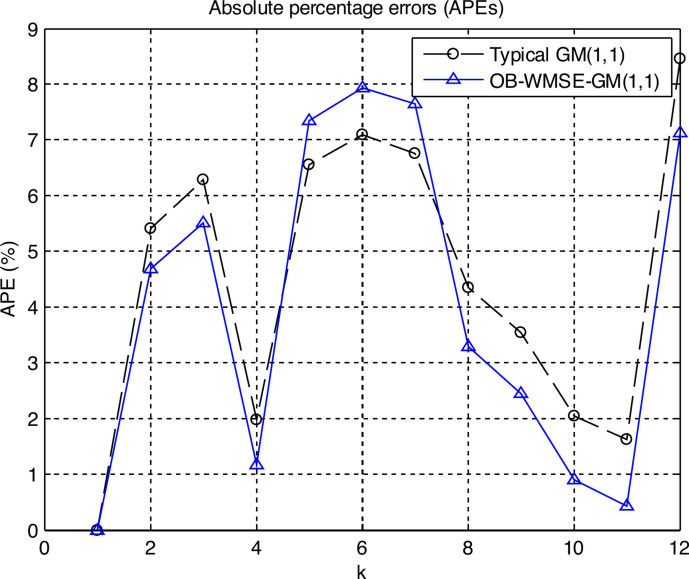
Figure 5 shows the graph of the APEs of the typical and proposed GM(1,1) models: Eqs. (26) and (27).
Fig. 5.
Graph of the APEs of the typical and proposed GM(1,1) models: Eqs. (26) and (27).
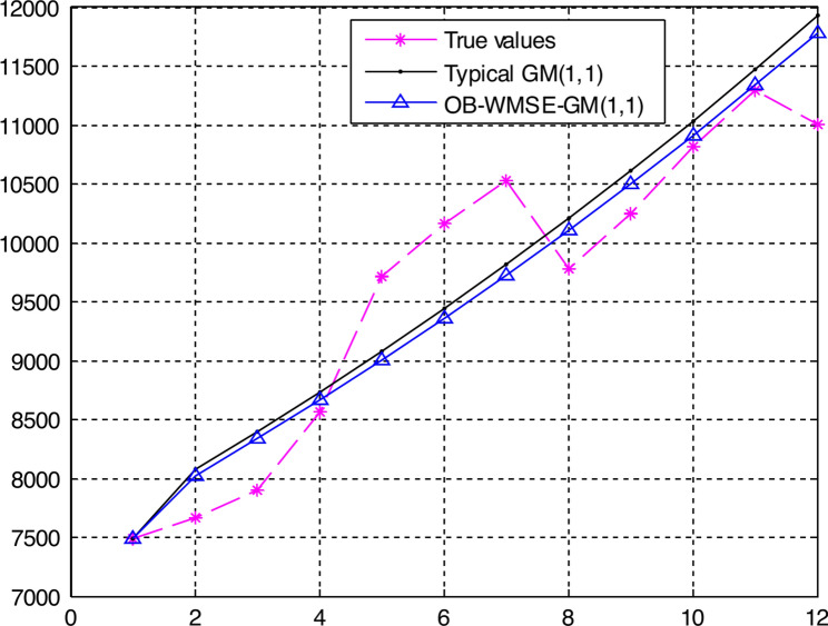
In Fig. 5 the points from k = 1 to k = 10 indicate the fitting points, and the points from k = 11 to k = 12 indicate the predicting points. Figure 6 shows the graph of the true values, fitting and predicting values of the typical and proposed GM(1,1) models: Eqs. (26) and (27).
Fig. 6.
Graph of the true values, fitting and predicting values of the typical and proposed GM(1,1) models: Eqs. (26) and (27).
Tables 5–6 and Figs. 5–6 numerically and visually illustrated that the fitting and predicting accuracy of the proposed OB-WMSE-GM(1,1) were significantly much higher than the typical GM(1,1).
Table 7 shows the fitting and predicting accuracy test results of the previous methods given in the Ref.3.
Table 7.
Fitting and predicting accuracy test results of the previous methods.
| k | Year | True value | Previous model 1: GA-Based GM(1,1) |
Previous model 2: GM(1,1;λ) with constrained linear least squares |
||
|---|---|---|---|---|---|---|
| Calculated value | APE (%) | Calculated value | APE (%) | |||
| 1 | 1983 | 7490 | 7490 | 0 | 7490 | 0 |
| 2 | 1984 | 7665 | 8052 | 5.048924 | 7914.36 | 3.253229 |
| 3 | 1985 | 7904 | 8370 | 5.895749 | 8224.29 | 4.052252 |
| 4 | 1986 | 8565 | 8700 | 1.576182 | 8546.36 | 0.21763 |
| 5 | 1987 | 9718 | 9444 | 2.81951 | 8881.05 | 8.612369 |
| 6 | 1988 | 10,164 | 9802 | 3.56159 | 9228.84 | 9.200708 |
| 7 | 1989 | 10,528 | 9983 | 5.176672 | 9590.25 | 8.9072 |
| 8 | 1990 | 9783 | 10,158 | 3.83318 | 9965.82 | 1.868752 |
| 9 | 1991 | 10,250 | 10,560 | 3.02439 | 10,356.09 | 1.035024 |
| 10 | 1992 | 10,815 | 10,977 | 1.49792 | 10,761.65 | 0.493296 |
| 11 | 1993 | 11,290 | 11,412 | 1.080602 | 11,183.09 | 0.946944 |
| 12 | 1994 | 11,000 | 11,946 | 8.6 | 11,621.03 | 5.645727 |
Table 8 shows the comparison result of the fitting and predicting MAPEs of the previous and proposed GM(1,1) models. As can be seen in Table 8, the proposed OB-WMSE-GM(1,1) has comparatively higher fitting and predicting performance. Especially, as can be seen in Table 8, the predicting APE at the first predicting year 1993 of the proposed GM(1,1) was 0.433388, and it was the first rank from among four models (1.628385, 0.433388, 1.080602, 0.946944). Consequently, we can evaluate that it is pretty superior to the APEs of the previous models 1 and 2.
Table 8.
Comparison of the fitting and predicting MAPEs of the previous and proposed GM(1,1) models.
| GM(1,1) | Fitting MAPEs (rank) | Predicting MAPEs (rank) |
|---|---|---|
| Typical GM(1,1) | 4.399448 (4) | 5.040509 (4) |
| Previous model 1: GA-Based GM(1,1) | 3.603791 (1) | 4.840301 (3) |
| Previous model 2: GM(1,1;λ) with constrained linear least squares | 4.182273 (3) | 3.296336 (1) |
| Proposed GM(1,1) | 4.090405 (2) | 3.775669 (2) |
The above results clearly demonstrated that the proposed OB-WMSE-GM(1,1) can significantly improve not only the fitting accuracy but also the predicting accuracy.
Conclusions
This paper proposed a new method to develop the improved GM(1,1) model based on weighted MSE and optimal weighted background value: OB-WMSE-GM(1,1), and verified its effectiveness by applying them to the simulation and application examples.
Conclusively, the following conclusions were drawn:
The main novelty of this work is to introduce the weighted accuracy evaluating metric: WMSE to improve the predicting accuracy of the GM(1,1), while all the previous GM(1,1) models have used the accuracy evaluating metrics with no weights (equal weights).
By selecting the appropriate optimal background weight, the accuracy of the GM(1,1) could be more and more improved.
The proposed OB-WMSE-GM(1,1) has not only excellent fitting accuracy but also excellent predicting accuracy.
The performance of the proposed OB-WMSE-GM(1,1) was significantly pretty higher than the typical GM(1,1).
By applying not only WMSE but also various techniques for improving the performance of the GM(1,1) such as original sequence pre-processing and smoothing, optimization of initial condition, reconstruction of background values, intelligent global optimization algorithms, rolling and metabolism mechanism, error compensation with residual GM(1,1) model, and combination of other modelling techniques, we can more and more improve the performance of the OB-WMSE-GM(1,1).
This work did not consider the problem to select more reasonable value of weighting factor r for improving the accuracy of the GM(1,1) owing to the limited space and time. Our future work will study such problem.
The proposed methods could be widely used to many prediction problems arising in practice.
Acknowledgements
This work was supported by Kim Chaek University of Technology, Democratic People’s Republic of Korea. The supports are gratefully acknowledged. The authors express their gratitude to the editors and the reviewers for their helpful suggestions for improvement of this paper.
Author contributions
Won-Chol Yang: Conceptualization, Methodology, Project administration, Supervision, Writing-original draft; Song-Chol Ri: Investigation, Methodology, Validation; Kyong-Su Ri: Methodology, Software, Writing-original draft; Chol-Ryong Jo: Data curation, Formal analysis; Jin-Sim Kim: Investigation, Validation, Visualization.
Funding
No funding has been received for this article.
Data availability
All data that support the findings of this study are included within this article.
Declarations
Competing interests
The authors declare no competing interests.
Ethics approval
The authors consent that the work carried out in this research is of high ethical standard. Moreover, this study does not include any human or animal subjects.
Consent to participate
Not applicable. This study does not have any participants, and hence, consent is not needed.
Footnotes
Publisher’s note
Springer Nature remains neutral with regard to jurisdictional claims in published maps and institutional affiliations.
References
- 1.Deng, J. L. Control problems of grey systems. Syst. Control Lett.1(5), 288–294 (1982). [Google Scholar]
- 2.Madhi, M. & Mohamed, N. An initial condition optimization approach for improving the prediction precision of a GM(1,1) mode. Math. Comput. Appl.22(21), 1–8. 10.3390/mca22010021 (2017). [Google Scholar]
- 3.Yeh, M. F. & Chang, M. H. GM(1,1;λ) with Constrained Linear Least Squares. Axioms10, 278. 10.3390/axioms10040278 (2021). [Google Scholar]
- 4.Tan, X. R. et al. A new GM (1,1) model suitable for short-term prediction of satellite clock bias. IET Radar Sonar Navig.16, 2040–2052. 10.1049/rsn2.12315 (2022). [Google Scholar]
- 5.Khan, A. M. & Osinska, M. Comparing forecasting accuracy of selected grey and time series models based on energy consumption in Brazil and India. Expert Systems With Applications212(118840), 1–16 (2023). [Google Scholar]
- 6.Yang, X. Y. Prediction of Medical Trauma Rehabilitation by GM (1,1) Model. Academic Journal of Science and Technology9(1), 241–244 (2024). [Google Scholar]
- 7.Shen, Y., Song, X. Y., Wang, X. S. & Han, S. A. Optimization and Application of GM(1,1) Model Based on Adams Formula. Journal of Physics: Conference Series1631(012115), 1–10. 10.1088/1742-6596/1631/1/012115 (2020). [Google Scholar]
- 8.Wang, Z. & Xu, S. Y. A Prediction Method of Ship Traffic Accidents Based on Grey GM(1,1) Model. Journal of Physics: Conference Series2381(012115), 1–7. 10.1088/1742-6596/2381/1/012115 (2022). [Google Scholar]
- 9.Qin, Y., Basheri, M. & Omer, R. E. E. Energy-saving technology of BIM green buildings using fractional differential equation. Applied Mathematics and Nonlinear Sciences7(1), 481–490. 10.2478/amns.2021.2.00085 (2022). [Google Scholar]
- 10.Guo, S. L., Wen, Y. H., Zhang, X. Q. & Chen, H. Y. Runoff prediction of lower Yellow River based on CEEMDAN-LSSVM-GM(1,1) model. Scientific Reports13, 1511. 10.1038/s41598-023-28662-5 (2023). [DOI] [PMC free article] [PubMed] [Google Scholar]
- 11.Shen, Q.Q.; Shi, Q.; Tang, T.P.; Yao, L.Q. A Novel Weighted Fractional GM(1,1) Model and Its Applications. Complexity, Volume 2020, Article ID 6570683, 1–20 (2020); 10.1155/2020/6570683.
- 12.Muksar, M. & Zuhri, S. Developing GM(3,1) Forecasting Model and Its Accuracy Compared to GM(1,1) and GM(2,1) Models. AIP Conference Proceedings2639(030003), 1–20. 10.1063/5.0111905 (2022). [Google Scholar]
- 13.Ma, X., Wu, W. Q. & Zhang, Y. Y. Improved GM(1,1) model based on Simpson formula and its applications. Journal of Grey System31(4), 33–46 (2019). [Google Scholar]
- 14.Wang, J. & Zhang, S. B. Deformation Prediction with weighted Grey GOM(1,1) Model and Time Series Method. Express Information of Mining Industry440(2), 25–27 (2006) ((in Chinese)). [Google Scholar]
- 15.Hikmah, N. & Kartikasari, N. D. Decomposition Method with Application of Grey Model GM(1,1) for Forecasting Seasonal Time Series. Pakistan Journal of Statistics and Operation Research18(2), 411–416 (2022). [Google Scholar]
- 16.Li, S., Cui, Du. H. & Q., Liu, P., Ma, X., Wang, H.,. Pipeline Corrosion Prediction Using the Grey Model and Artificial Bee Colony Algorithm. Axioms11, 289. 10.3390/axioms11060289 (2022). [Google Scholar]
- 17.Liu, J. F. & Yang, R. R. Application of metabolic GM (1,1, th, p) power model in fresh e-commerce prediction. SHS Web of Conferences166, 01064. 10.1051/shsconf/202316601064 (2023). [Google Scholar]
- 18.Mi, C. M. et al. Seasonal electricity consumption forecasting: an approach with novel weakening buffer operator and fractional order accumulation grey model. Grey Systems: Theory and Application14(2), 414–428. 10.1108/GS-08-2023-0074 (2024). [Google Scholar]
Associated Data
This section collects any data citations, data availability statements, or supplementary materials included in this article.
Data Availability Statement
All data that support the findings of this study are included within this article.


