

Abstract
The Marine Predator Algorithm (MPA) has unique advantages as an important branch of population-based algorithms. However, it emerges more disadvantages gradually, such as traps to local optima, insufficient diversity, and premature convergence, when dealing with complex problems in practical industrial engineering design applications. In response to these limitations, this paper proposes a novel Improved Marine Predator Algorithm (IMPA). By introducing an adaptive weight adjustment strategy and a dynamic social learning mechanism, this study significantly improves the encounter frequency and efficiency between predators and preys in marine ecosystems. The performance of the IMPA was evaluated through benchmark functions, CEC2021 suite problems, and engineering design problems, including welded beam design, tension/compression spring design, pressure vessel design, and three-bar design. The results indicate that the IMPA has achieved significant success in the optimization process over other methods, exhibiting excellent performance in both solving optimal parameter solutions and optimizing objective function values. The IMPA performs well in terms of accuracy and robustness, which also proves its efficiency in successfully solving complex industrial engineering design problems.
Keywords: Improved marine predators algorithm, Self-adaptive weight, Social strategy, Complex industrial engineering design problems
Subject terms: Engineering, Mathematics and computing
Introduction
Optimization problems are prevalent in scientific research and engineering applications such as financial management, energy scheduling, path planning, engineering design, and sensor network Optimization. These applications have drawn a great deal of attention from academics in related fields. In most scientific research as well as technical applications, the primary research direction is how to tackle optimization problems with the least amount of resources. Numerous new technologies are being developed and applied widely, which is leading to the continuous emergence of more complicated optimization challenges. Optimization issues have more variables, a wider solution scale, and more complexity than the prior single constraints. The complexity of the variable's dimensionality often increases exponentially for single-objective continuous optimization problems, multi-objective continuous optimization issues, and discrete optimization problems. To solve discrete optimization problems more effectively, the majority of currently available algorithms must be discretized because they are designed for continuous optimization, which makes it challenging to apply them directly to discrete optimization problems. As a result, to tackle optimization challenges, better algorithms must be created for each unique situation.
Optimization algorithms have garnered significant attention and in-depth study from researchers across fields very quickly. The majority of intelligent optimization algorithms are developed through animal simulations and the analysis of diverse creatures' communication patterns. The mayfly algorithm, which was proposed by Zervoudakis et al.1 and is inspired by the flight behavior and mating process of mayflies, is one of the novel representative algorithms. Mohammadi-Balani et al.2 proposed an algorithm based on the hunting spiral of a golden eagle by observing its speed in the golden eagle optimization algorithm is proposed by observing the way the golden eagle adjusts its speed at different stages of the trajectory. Yuan et al.3proposed a prevention-inspired bionic optimization algorithm, named Coronavirus Mask Protection Algorithm (CMPA) based on the virus transmission of COVID-19. In CMPA, the process of infection and immunity consists of three phases, including the infection stage, diffusion stage, and immune stage. Kaveh et al.4 simulated the territorial behavior of water striders, ripple communication, mating mode, feeding mechanism, and succession proposed the water strider algorithm. Chou et al.5 observed the pattern of jellyfish movements following the currents and in the jellyfish swarms, and by simulating the temporal control mechanism of switching between these movements as well as the process of converging into jellyfish blooms propose an artificial jellyfish search algorithm. Yuan et al.6 proposed a learning-imitation strategy-assisted alpine skiing optimization (LISASO). In LIS, the learning ability of individuals and the imitation of competitions are introduced to strengthen the association between individuals and the first individual. Yuan, YL; Ren, JJ[7]proposed a novel swarm intelligence optimization algorithm is proposed, which is named alpine skiing optimization (ASO). The main inspiration for the ASO originated from the behaviors of skiers competing for the championship.
The study and proposal of new algorithms with better performance are of great importance to the research of intelligent Optimization algorithms and the improvement of the theoretical system. The Marine Predator Algorithm (MPA) is a new intelligent Optimization algorithm proposed by Mirjalili et al.8 based on the foraging pattern of marine organisms. The Marine Predator Algorithm, which has the benefits of a simple structure, few parameters, and ease of implementation, solves the optimization problem by mimicking the laws of marine organisms foraging for prey, including sharks, toucans, sunfish, and swordfish. However, MPA presents weak points towards premature convergence, stuck into local optima, and lack of diversity, specifically, which is in the real-world niche problems within different industrial engineering design domains.
To get rid of such limitations, this paper presents an Improved Marine Predators Algorithm (IMPA) to mitigate above mentioned limitations by deploying the self-adaptive weight and dynamic social learning mechanism. IMPA can find an approximate optimal solution relatively quickly by combining dynamic social strategies and adaptive weight settings, and overcome limitations by avoiding local optimal solutions and improving overall performance. IMPA promotes balanced exploration and exploitation through dynamic social strategies and adaptive weights. The proposed method achieves enhanced solution quality, maintained population diversity, and accelerated convergence speed.
Background and related work
Since the traditional MPA was initially presented in 2020, several MPA versions have been put up for a wide range of optimization issues. Binary, discrete, modified, hybridized, chaotic, quantum and multi-objective MPA versions are the different classifications for these MPA variations. Abdel-Basset et al.9 created the IMPA to solve multi-threshold medical image segmentation. This approach improves the particles that fail to find a workable solution after a certain number of iterations by adding a ranking-based diversity reduction (RDR) mechanism to the traditional MPA. To detect COVID-19, the model utilized in this study operates on chest X-ray pictures. The experiment findings demonstrate that the IMPA provides higher-quality segmented images than other algorithms when compared against a wide range of other metaheuristics.
The IMPOA is suggested by Shaheen et al.10 as a solution to the CHP issue. By improving predator techniques that take environmental and climatic variation into account, IMPOA maintains a balance between the exploitation and exploration phases. Several limitations are taken into consideration when solving the CHP issue using the suggested technique. Test systems including 5, 48, 84, and 96 units were used to assess the IMPOA's efficacy. The simulation's findings demonstrate the IMPOA's superiority in terms of stability and pace of convergence.
In Yu et11, an adaptive MPA (AMPA) is presented as a way to minimize load demands by optimizing the configuration of a hybrid power system integrating batteries, PV, and diesel generator. Three objective functions, including the annualized cost, the value of CO2 emissions, and the chance of load loss for the hybrid power generation system, are minimized in this multi-objective optimization problem. The AMPA is compared with LOA, FOA, COA, and conventional MPA and validated on multiple benchmark functions. The simulation findings validate AMPA's best accuracy and fastest convergence. Shaheen, El-Sehiemy, et al.12 offer an improved MPA to address simultaneous distribution reconfiguration with distribution generations. The suggested method accounts for differences in the temperature and environment. The prey's new positions are updated in EMPA using a random probability. The voltage stability index (VSI) is improved and power losses are minimized using the suggested algorithm under different loading scenarios. EMPA's performance was evaluated using IEEE 33, 83, and 137-bus distribution networks. Compared to other competing algorithms, the EMPA produces better results by efficiently minimizing the problem under consideration.
In Yang et al.13, multi-strategy marine predators algorithm-joint regularized is a semi-supervised classification model. Machine Learning with Applications semi-supervised extreme learning machine (MSMPA) is built. MSMPA incorporates supervised information regularization and is based on Hessian regularization. MSMPA uses several techniques to enhance its functionality. To create a high-quality initial population for the MSMPA, a chaotic opposition learning strategy is applied during initialization. In each of the three stages of the MSMPA, adaptive inertia weights and adaptive step control factors are used to improve local optimal prevention, convergence speed, and exploration and exploitation capabilities. The simulation studies show that MSMPA exhibits better classification accuracy and stability than other competitive classification approaches.
In Houssein, Hassaballah et al.14, a novel nonlinear step factor control method is utilized to balance the exploration and exploitation stages, increase the pace of convergence, and improve the MPA's capacity for global search. Convolutional Neural Networks (CNNs) and the suggested IMPA are combined for the categorization of electrocardiograms (ECGs). The resulting model, dubbed IMPA-CNN, is tested on the European ST-T database, the St. Peters-burg INCART database, and the MIT-BIH arrhythmia database. The experimental results indicate the superiority of the IMPA-CNN models compared to MPA, GSA-NN, EO-CNN, HHOCNN, SCA-CNN, PSO-CNN, and WOA-CNN models using multiple assessment metrics.
In Liu et al.15, the MPA is combined with a novel predator encoding mechanism based on internet protocol (IP) to create an IPMPA algorithm. A deep convolutional neural network (DCNN) and the suggested IPMPA are merged to create a new model called DCNN-IPMPA, which is used for COVID-19 diagnosis. We evaluate the DCNN-IPMPA's performance using the COVID-CT and SARS-CoV-2 datasets. The outcomes of the simulation demonstrate that the DCNN-IPMPA model outperforms other models in terms of results.
Yuan et al.16 presented a novel assisted optimization strategy, named elite opposition-based learning and chaotic k-best gravitational search strategy (EOCS), which is proposed for the grey wolf optimizer (GWO) algorithm. In the EOCS-based grey wolf optimizer (EOCSGWO) algorithm, the elite opposition-based learning strategy (EOBLS) is proposed to take full advantage of better-performing particles for optimization in the next generations.
Aydemir, S. B[17]proposed a dynamic selection strategy named as FOCLMPA that adapts during the evolutionary process. This dynamic approach assigns higher selection probabilities to parents with superior fitness, resulting in accelerated convergence and heightened exploration capabilities. They innovatively suggested a dynamic dimension and a greedy strategy by dimension approach. This strategy evaluates solutions in each dimension, mitigating the risk of local optima, thereby enhancing the overall performance of the algorithm.
Du and Guo18ventured into hybridization named as EMPA by combining the Marine Predators Algorithm with opposition-based learning. This hybrid approach combines opposing initial numbers with a self-adaptive component strategy, effectively liberating the algorithm from local optima traps and facilitating superior convergence. These include opposition learning to expand the search range, adaptive evolution for heightened global exploration, neighborhood search to diversify the population, and greedy selection to ensure solution quality.
Han and Du19 presented a modification to the MPA algorithm by adjusting conversion parameters. This adjustment transitions from a linear decline to a nonlinear one, optimizing the balance between global and local exploration. They put forward a hybrid algorithm seamlessly integrating the exploitation capabilities of crossover with individual solutions' personal best states, self-learning mechanisms, and global search mechanisms. This algorithm updates solutions using sine or cosine strategies, implementing a novel approach to mutualism phases.
Kumar et al.20 have demonstrated the remarkable prowess of MPA in addressing multi-objective problems related to real-time task scheduling within multiprocessor systems, underscoring its relevance in the realm of computational optimization.
Nonetheless, like so many other metaheuristics, the MPA exhibits some disadvantages due to its numerous decision variables, dense local optimal solutions, and high computational effort. The Marine Predator Algorithm will converge to the local optimal position in the space, stretching from the current number to the opposite number which has made less progress in handling high-dimensional optimization problems than the majority of the aforementioned research. For this purpose, The processes for the development of the Improved Marine Predators Algorithm (IMPA) with self-adaptive weight and dynamic social strategy have been performed. The motivation for this article is listed below.
Self-adaptive weight parameter tuning scheme is adopted into the IMPA. according to the proportion of fitness value;
Dynamic Social Mechanism was implemented to balance exploration and exploitation, preventing premature convergence to a local optimal position;
The proposed algorithm was tested by 23 benchmark test functions and IEEE CEC 2021 benchmark, compared to state-of-the-art algorithms and different MPA variants.
The proposed algorithm was tested on four different real-world engineering problems and compared with some algorithm in the literature.
The remaining part of this paper is organized as follows. Section "Marine Predators Algorithm" describes the Marine Predators Algorithm. Section "Improved Marine Predators Algorithm" describes the Improved Marine Predators Algorithm in detail. Section "Experiments and discussion" gives the experimental results and analysis of the benchmark function. Section “Engineering design optimization” examined the IMPA in engineering problems. Section “Conclusion” concludes this paper and indicates future research.
Marine predators algorithm
The Marine Predators Algorithm (MPA) operates as a population-based algorithm, a characteristic shared with other metaheuristic algorithms. One of its distinctive features involves periodically disseminating the initial solution across the search space for initial demonstration purposes, as expressed in the following equation in Eq. (1):
| 1 |
Rand represents a random vector between 0 and 1, while and denote the lower and upper bounds of the parameters being optimized. This initial dispersion of solutions sets the stage for subsequent optimization steps. In the context of MPA, the best solution discovered is identified as the dominant Predators, and it plays a pivotal role in the creation of a matrix known as Elite, as depicted in Eq. (2). These matrices are instrumental in tracking and locating prey, relying on the positional information of the prey itself.
| 2 |
For the Elite matrix, represents the best predators vector, where n corresponds to the number of Predators, and d is the number of dimensions. The Elite matrix undergoes updates when a superior agent replaces the best predators. The Prey matrix, on the other hand, shares a similar dimensionality with the Elite matrix. Agents in pursuit of prey adjust their positions based on the information contained within the Prey matrix. Therefore, the initialization phase is pivotal in generating the initial Prey matrix, with the best predators being responsible for creating the Elite matrix. Equation (3) provides an expression for the Prey matrix.
| 3 |
In essence, the entire optimization process in MPA hinges on the interactions and dynamics governed by the Prey and Elite matrices, encapsulating the algorithm's unique approach to problem-solving. There are three phases in the MPA’s optimization process:
Phase 1—High Velocity Ratio (HVR): This initial phase occurs when the prey's speed falls below that of the predators, emphasizing the importance of exploration in the early stages of optimization. The mathematical representation of this phase is given by in Eq. (4):
While Iteration < 1/3 × max(Iteration)
| 4 |
represents the Brownian Motion utilizing a regularly distributed random vector. The symbol ⊗ denotes entry-wise multiplications, simulating the prey's motion via the multiplication of . The phase introduces two variables: a constant number P and a vector of random values R ranging from 0 to 1.
Phase 2—Uniform Velocity Ratio (UVR): In this phase, both prey and predators move at comparable speeds, necessitating a balance between exploration and exploitation. Half of the agents are assigned to exploration, and the other half to exploitation, with both predators and prey sharing these responsibilities. The mathematical representation during this phase is as follows:
While 1/3 × max(Iteration) < Iteration < 2/3 × max(Iteration)
The first half of searching agents in Eq. (5)
| 5 |
is a randomly generated vector based on Levy Flight (LF). It simulates prey movement by adding prey location to the step size. The MPA posits that the other 50% of the population follows the rules outlined in Eq. (6).
| 6 |
Phase 3—Low Velocity Ratio (LVR): This stage occurs when the prey moves more slowly than the predators and is defined as in Eq. (7) :
While Iteration > 2/3 × max(Iteration)
| 7 |
Eddy formation or Fish Aggregation Devices (FADs), which can impact the algorithm's behavior. These factors are considered as local optima avoidance operators and influence the optimization process. Longer hops during simulation are considered to minimize stagnation in local optima. The impact of FADs is outlined as follows in Eq. (8):
| 8 |
These phases and adaptive strategies define the dynamics of the MPA, which is presented in Fig. 1. They are enabling it to navigate the optimization landscape efficiently while addressing different scenarios and challenges.
Figure 1.

Marine Predators Algorithm.
Improved Marine Predators Algorithm
Self-adaptive Weight
In this paper, we provide a novel optimization method that includes an adaptive weight parameter in the process. By harnessing the adaptive nature of this parameter, our approach enhances the algorithm's global exploration capability and its ability to escape local optima, all while maintaining strong performance in local refinement when optimization conditions stabilize. Specifically, during the initial stages of optimization, our approach accelerates global exploration of the solution space. As the optimization process stabilizes, it shifts focus toward local solution development, achieving a balance between global and local exploration. To achieve this, we leverage the positional information of the destination point through the design of a self-adaptive weight position-update mechanism, denoted as Eq. (9)-Eq. (12):
While Iteration < 1/3 × max(Iteration)
| 9 |
While 1/3×max(Iteration)<Iteration<2/3×max(Iteration)
| 10 |
While Iteration > 2/3 × max(Iteration)
| 11 |
| 12 |
It is difficult to tune the model and find a suitable weight parameter, ω. We want to minimize the function of our model by changing the weight parameters. Bayesian optimization helps us to find the most suitable point for the weighting parameter in the fewest number of steps. Bayesian optimization also uses an Acquisition Function21, which directs the sampling to regions that are likely to be better than the current best observation. The Acquisition Function, brought into the model, picks the best performing parameters. The tuning is cross-validated by the Grid Search CV22, which iterates through all permutations of the incoming parameters and returns the evaluation metrics scores for all parameter combinations by means of cross-validation.
Our enhanced approach replaces premature convergence, which improves the subpar search capability observed. The weight parameter, denoted as ω, is a self-adaptive balancing factor. In this study, we propose a self-adaptive weight ω that guides dynamic correction within the update formula, where represents the best fitness value of the current iteration for the position variable and signifies the global optimal fitness value. Its function is to dynamically adjust the weight between the destination point and the current individual's position.
When the fitness value of the current position variable surpasses the global fitness value, the inertia weight assumes a higher value, which enhances global exploration capabilities and expands the search space for feasible solutions. Conversely, the self-adaptive weight generates a smaller value, promoting faster convergence rates and facilitating local refinement. The self-adaptive weight plays a critical role in enabling particles within the MPA to autonomously select between global and local phases, thereby enhancing accuracy and reducing the likelihood of falling into local optima.
Dynamic social strategy
In this section, we introduce another critical element of the Improved Algorithm, which balances the potential neighborhood information of Elite Predators with that of other individuals and employs it to enhance the MPA. This provides more effective updates for the optimal individuals, reducing the probability of falling into local optima and attempting to overcome premature convergence. This significantly increases the probability of the population reaching the global optimum, thereby enhancing the development capacity.
This dynamic social strategy optimizes the search space and accelerates the effectiveness of the search process in the IMPA. The modified search mechanism introduced in the IMPA is expressed as follows:
While Iteration < 1/3 × max(Iteration)
| 13 |
While 1/3 × max(Iteration) < Iteration < 2/3 × max(Iteration)
| 14 |
While Iteration > 2/3 × max(Iteration)
| 15 |
In this optimization methodology, The second crucial component in the search process is the social component, denoted as , which improves the ability to develop solutions locally while still maintaining the ability to escape from local optima. When the search area provided by the coefficient is very large, the updated solution may diverge from the current state to avoid falling into local optima.
This dynamic social component amalgamates with the self-adaptive weight, collectively providing guidance to the current solution. By combining the directional influence of the best solution state and the best population state, the newly developed algorithm encompasses the following steps:
Pseudocode.
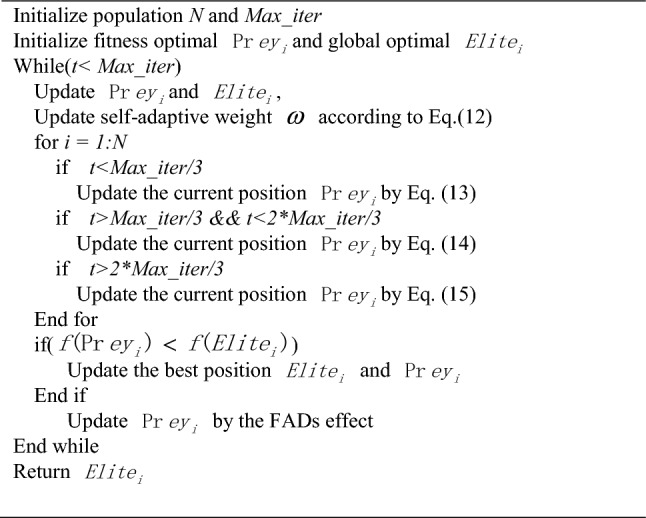
The Improved Marine Predators Algorithm.
As the parameters of the IMPA is concerned, N is the population , D is the dimension and Max_iters is Number of iterations. The time complexity of setting the adaptive weight and Dynamic Social Strategy is O(N·D).The time complexity of IMPA is O(N·D·Max_iter), which is the same as that of the origin MPA algorithm, indicating that the two improved strategies do not increase the computational burden of the Marine Predator Algorithm.
Our improved algorithm introduces a random selection mechanism for self-adaptive weight and dynamic social strategy, ensuring a harmonious balance between predators and prey position updates. Self-adaptive weight parameter tuning scheme is adopted into the IMPA, according to the proportion of fitness value. Dynamic social mechanism was implemented to balance exploration and exploitation, preventing premature convergence to a local optimal position. This comprehensive approach, which combines dynamic weight adaptation and social strategy, significantly enhances the optimization capabilities of the IMPA, improving its performance across a range of optimization problems. Thus the phase of opposition based weight and self-adaptive strategy provides an enhanced global and local search which helps in increasing appropriate diversity and avoids the skipping of true solutions. The flow of search process of proposed IMPA is presented in Fig. 2 A detailed analysis off enhanced diversity of solutions and exploitation of search space has been done in experimental section.
Figure 2.

Framework of IMPA.
Experiments and discussion
Benchmark Problem Experiments
In the realm of optimization research, a fundamental aspect of assessing the effectiveness of newly proposed algorithms lies in the rigorous evaluation process employed. In this context, our study undertakes a comprehensive examination of the IMPA across a diverse range of benchmark problems. These benchmark functions, numbering 23 in total, are categorized into three distinct classes: unimodal, multimodal, and fixed-dimension problems23,24.
For the evaluation of these classical problems, a population size of 50 solutions was employed with a uniform termination criterion of 1000 iterations applied to all algorithms, whose dimensions are set up to 50. To ensure the robustness and reliability of our findings, a thorough comparative analysis was conducted based on two evaluation criteria: the mean and standard deviation. This evaluation was carried out through 20 independent runs on each benchmark function, yielding a comprehensive assessment of the algorithm's efficacy. Experimental computations were executed using MATLAB 2020a on a personal computer equipped with a 3.2 GHz CPU and 16 GB RAM.
The proposed method must show its competitive performance over some of those truly state-of-the-art methods. The results of our study reveal that the IMPA exhibits superior optimization performance compared to the MPA and several of the most recently proposed state-of-the-art methods algorithms, including Rime Optimization Algorithm (RIME)25, African Vultures Optimization Algorithm (AVOA)26, Artificial Gorilla Troops Optimizer (GTO)27, Optical Microscope Algorithm (OMA)28and Improved Sine Cosine Algorithm (IWSCA)29. Furthermore, this section includes a comparative analysis with some improved versions of MPA, specifically Enhanced MPA (EMPA)30 and Gradient-Descent-based MPA (GDMPA)31. The detailed results of this comparative assessment are presented in Table 1.
Table 1.
Comparison results for benchmark functions.
| RIME | AVOA | GTO | OMA | IWSCA | MPA | EMPA | GDMPA | IMPA | ||
|---|---|---|---|---|---|---|---|---|---|---|
| F1 | Mean | 1.83E+00 | 0* | 0* | 73,711.65976 | 2.0325E−305 | 1.10586E−45 | 9.551725 | 73,926.97 | 0* |
| Std | 0.033687241 | 0* | 0* | 103,280.8621 | 0 | 1.47981E−45 | 12.23421 | 17,189.45 | 0* | |
| F2 | Mean | 2.48E+00 | 0* | 0* | 8.22018E+30 | 5.0237E−149 | 7.15291E−27 | 1.659189 | 2.35E+13 | 0* |
| Std | 0.177327304 | 0* | 0* | 1.16251E+31 | 6.3254E−149 | 6.43065E−27 | 1.124542 | 3.01E+13 | 0* | |
| F3 | Mean | 4.82E+03 | 0* | 0* | 311,140.7274 | 3.12E−285 | 4.62262E−08 | 16,277.87 | 101,277.1 | 0* |
| Std | 1420.11283 | 0* | 0* | 437,620.7511 | 0 | 6.4216E−08 | 2627.994 | 15,784.57 | 0* | |
| F4 | Mean | 1.73E+01 | 0* | 0* | 74.25635165 | 1.6394E−157 | 1.61174E−17 | 0.311318 | 69.86455 | 0* |
| Std | 0.348893943 | 0* | 0* | 36.30472632 | 2.3185E−157 | 1.74054E−18 | 0.10907 | 1.301586 | 0* | |
| F5 | Mean | 3.13E+02 | 2.79E−05* | 43.92575 | 316,890,837.4 | 4.81765E−05 | 43.1203333 | 133.2982 | 2.84E+08 | 2.29769E−05 |
| Std | 74.50977091 | 3.88E−05* | 0.305613 | 448,018,563 | 6.62317E−05 | 0.085618377 | 119.5431 | 10,878,301 | 2.46087E−05 | |
| F6 | Mean | 2.40E+00 | 2.13E−08 | 0.037744 | 79,512.904 | 0.04510626 | 2.62536E−08 | 1.900509 | 78,735.79 | 7.63259E−10* |
| Std | 1.516431193 | 2.91E−09 | 0.045125 | 111,396.0966 | 0.034909693 | 6.15778E−09 | 0.583362 | 3349.898 | 1.06888E−09* | |
| F7 | Mean | 3.87E−02 | 1.13E−05 | 2.13251E−05 | 246.203361 | 0.000117546 | 0.001040433 | 0.100476 | 180.8921 | 4.35E−06* |
| Std | 0.011201032 | 9.32E−06 | 8.09298E−06 | 346.3149937 | 0.000148561 | 0.000655853 | 0.0712 | 0.19872 | 6.05E−06* | |
| F8 | Mean | −1.72E+04 | −13,021.3 | −20,949.14436 | −3712.911898 | −7174.099901 | −15,551.89182 | −11,583.9 | −7865.45 | −2.09E+04* |
| Std | 24.60148659 | 242.4315 | 3.49852E−10 | 5026.223273 | 249.3668736 | 191.9082888 | 371.0039 | 671.9733 | 4.26E−07* | |
| F9 | Mean | 0* | 3.04E+01 | 0* | 0* | 1007.907608 | 0* | 69.13439 | 599.6754 | 0* |
| Std | 0* | 4.99079528 | 0* | 0* | 72.52931792 | 0* | 19.03083 | 56.75393 | 0* | |
| F10 | Mean | 1.91E+00 | 8.88E−16 | 8.88178E−16 | 16.33314408 | 8.88178E−16 | 4.44089E−15 | 1.6573 | 17.78133 | 8.88E−16* |
| Std | 0.286164829 | 0 | 0 | 6.902385394 | 0 | 0 | 1.403677 | 0.316152 | 0* | |
| F11 | Mean | 8.12E−01 | 0* | 0* | 882.3145682 | 0* | 0* | 0.081999 | 391.6581 | 0* |
| Std | 0.002075913 | 0* | 0* | 1243.775962 | 0* | 0* | 0.094563 | 11.37449 | 0* | |
| F12 | Mean | 5.38E+00 | 4.68E−10 | 0.022478 | 721,570,701.2 | 0.001656308 | 2.0154E−09 | 0.015901 | 5.36E+08 | 5.52733E−11* |
| Std | 1.759051378 | 3.13E−10 | 0.012132 | 1,020,454,988 | 0.00094689 | 1.06642E−10 | 0.001225 | 21,710,845 | 7.00712E−11* | |
| F13 | Mean | 4.97E−01 | 3.88E−09 | 0.117997 | 1,422,848,975 | 4.38298E−07 | 2.7927E−08 | 0.051358 | 1.04E+09 | 2.12751E−09* |
| Std | 0.214264812 | 3.44E−10 | 0.160096 | 2,012,158,438 | 6.14402E−07 | 6.97689E−09 | 0.030578 | 13,698,206 | 2.90836E−09* | |
| F14 | Mean | 3.46E+00 | 9.98E−01 | 3.950756354 | 261.9782921 | 7.951564594 | 0.998003838 | 4.507942 | 6.163716 | 0.998004* |
| Std | 3.486631297 | 4.71E−16 | 4.175822655 | 336.6126789 | 6.67359067 | 0 | 2.134801 | 2.461043 | 0* | |
| F15 | Mean | 1.10E−02 | 4.00E−04 | 0.000542792 | 0.959327936 | 0.002699257 | 0.000307486 | 0.002224 | 0.001735 | 0.000307* |
| Std | 0.013212518 | 5.78E−05 | 0.00017189 | 1.324822465 | 0.002464541 | 3.83323E−19 | 0.00033 | 0.000633 | 7.67E−20* | |
| F16 | Mean | −1.03E+00 | −1.03E+00 | −1.031248995 | 321.9470001 | −0.984958941 | −1.031628453 | −1.01995 | −1.02442 | −1.03163* |
| Std | 1.02809E−07 | 2.23E−12 | 0.000487899 | 455.6062817 | 0.063957969 | 0 | 0.006994 | 0.009946 | 0* | |
| F17 | Mean | 3.98E−01 | 3.98E−01 | 0.497658429 | 4.200093154 | 0.402981939 | 0.397887358 | 0.437015 | 0.413355 | 0.397887* |
| Std | 3.56092E−05 | 1.26E−15 | 0.138064149 | 5.342065731 | 0.005560347 | 0 | 0.017909 | 0.021466 | 0* | |
| F18 | Mean | 4.61E+01 | 1.65E+01 | 17.60271856 | 115.6570207 | 25.20217481 | 3 | 3.300957 | 3.536866 | 3* |
| Std | 60.95042098 | 1.91E+01 | 20.63516026 | 112.6090904 | 7.155485643 | 0 | 0.13192 | 0.496593 | 0* | |
| F19 | Mean | −3.86E+00 | −3.86E+00 | −3.862772367 | −3.666673049 | −3.834087963 | −3.862782148 | −3.85669 | −3.82952 | −3.86278* |
| Std | 9.14435E−07 | 1.61E−05 | 1.35031E−05 | 0.2766239 | 0.004224394 | 0 | 0.000615 | 0.027548 | 0* | |
| F20 | Mean | −3.32E+00 | −3.26E+00 | −3.322 | −1.887759676 | −3.064140909 | −3.321995172 | −2.95493 | −2.90161 | −3.262548611* |
| Std | 1.01605E−05 | 8.44E−02 | 2.51E−15 | 2.027932031 | 0.0644847 | 2.22045E−15 | 0.102336 | 0.012301 | 0.084070132* | |
| F21 | Mean | −3.87E+00 | −1.02E+01 | −10.15319967 | −3.20572885 | −10.10327247 | −10.15319968 | −7.15709 | −2.88735 | −10.1532* |
| Std | 1.746735607 | 1.04E−07 | 6.67166E−09 | 4.367303045 | 0.055574157 | 1.77636E−15 | 3.322242 | 0.220971 | 1.78E−15* | |
| F22 | Mean | −1.04E+01 | −1.04E+01 | −10.40294057 | −4.44037456 | −10.36647304 | −10.40294057 | −4.65739 | −4.27223 | −10.4029* |
| Std | 0.001170383 | 3.19E−09 | 3.06354E−10 | 6.00658441 | 0.048483391 | 0 | 2.28222 | 0.029231 | 0* | |
| F23 | Mean | −1.05E+01 | −8.67E−01 | −1.05E+01 | −10.53640979 | −0.22686473 | −10.52977601 | −5.29647 | −3.33951 | −10.5364* |
| Std | 0.00E+00 | 0.228671286 | 7.95E−08 | 3.97204E−08 | 0.066386287 | 0.001101293 | 1.605098 | 0.205943 | 3.97E−15* |
*Represent the optimal solution of the function.
In our comparative analysis, we examined the experimental results of various algorithms applied to the F1-F23 functions. The IMPA consistently attained the theoretical global optimum for 22 out of the 23 functions (F1-F4, F6-F23). Among the F1-F4 functions, the improved algorithm AVOA, and GTO algorithm can obtain the optimal solution, but the IMPA has better experimental results in other functions except for F5. The experiment shows that the improved algorithm performs better results in the remaining results.
The comparative performance of RIME, OMA, and IWSCA fell short when compared to the exceptional performance of the IMPA across all 23 benchmark functions. Notably, the IMPA surpassed other improved versions of MPA, such as EMPA and GDMPA. These findings underscore IMPA's superior performance in terms of global exploration capabilities and its ability to evade local optima in comparison to the other algorithms.
This study additionally presents the convergence curves for the nine optimization algorithms refer to Fig. 3. The results indicate that the IMPA excels in reaching the theoretical global minimum for the Unimodal functions (F2-F4), achieving this within approximately 400 to 500 iterations. For the Multimodal functions (F9-F11), the IMPA also exhibits faster convergence than other algorithms, reaching the theoretical global minimum in 100 iterations. Even in the context of fixed-dimension problems, the IMPA demonstrates superior convergence speed and accuracy relative to other algorithms, highlighting its distinctive characteristics.
Figure 3.

Convergence curves for benchmark functions.
Conversely, the other algorithms consistently experience premature convergence across all benchmark functions, yielding solutions consistently inferior to those of IMPA. Although MPA and GTO perform better than IMPA in only two functions (F1 and F5), they lag behind in other scenarios. The convergence curves clearly demonstrate that IMPA consistently reaches the theoretical global minimum for most benchmark functions, underscoring its superior optimization performance. The outstanding convergence speed of IMPA significantly reduces the computational complexity of the optimization problem.
This study additionally presents the convergence curves for the nine optimization algorithms refer to Fig. 3. The results clearly indicate that the IMPA excels in reaching the theoretical global minimum for the Unimodal functions (F2-F4), achieving this within approximately 400 to 500 iterations. For the Multimodal functions (F9-F11), the IMPA also exhibits faster convergence than other algorithms, reaching the theoretical global minimum in 100 iterations. Even in the context of fixed-dimension problems, the IMPA demonstrates superior convergence speed and accuracy relative to other algorithms, highlighting its distinctive characteristics.
Conversely, the other algorithms consistently experience premature convergence across all benchmark functions, yielding solutions consistently inferior to those of IMPA. Although MPA and GTO perform better than IMPA in only two functions (F1 and F5), they lag behind in other scenarios. The convergence curves clearly demonstrate that IMPA consistently reaches the theoretical global minimum for most benchmark functions, underscoring its superior optimization performance. The outstanding convergence speed of IMPA significantly reduces the computational complexity of the optimization problem.
In order to illustrate whether there are differences between the IMPA and the comparison algorithm, Wilcoxon rank-sum test23 and Friedman test are also introduced to analyze the results of the algorithm, which are presented in Tables 2 and 3. The significance p-value is set to 0.05, When the p-value in the Wilcoxon rank-sum test is less than 0.05, it means that there is a significant difference between the algorithm proposed in this article and the comparison algorithm. Otherwise, it means that there is no significant difference between the algorithm in this article and the comparison algorithm. In the result table, ‘+’ denotes the IMPA is better than another counterpart, ’ -’ means other algorithms are better, and ’NAN’ means there is no significant difference between the two algorithms after the test. The results show that the p-value of the OMA and the GTO on the function is greater than 0.05, indicating that there is no significant difference between the two algorithms and the IMPA. In addition, the p-value of the IMPA is less than 0.05, indicating that there is a significant difference between the IMPA and other comparison algorithms. it is obvious that the IMPA performs better than other algorithms, and the improvement strategy introduced in the IMPA is effective.
Table 2.
Wilcoxon rank-sum test.
| IMPA | |||||||||||||||||||||||
|---|---|---|---|---|---|---|---|---|---|---|---|---|---|---|---|---|---|---|---|---|---|---|---|
| F1 | F2 | F3 | F4 | F5 | F6 | F7 | F8 | F9 | F10 | F11 | F12 | F13 | F14 | F15 | F16 | F17 | F18 | F19 | F20 | F21 | F22 | F23 | |
| RIME | + | + | + | + | + | NAN | + | + | + | + | + | + | + | + | + | + | NAN | + | + | + | + | + | + |
| AVOA | + | + | + | + | + | + | + | + | + | + | NAN | + | + | + | + | + | + | + | + | + | + | + | + |
| GTO | − | − | − | − | NAN | − | − | − | − | − | − | − | − | − | − | NAN | − | − | − | − | − | − | − |
| OMA | − | − | − | − | − | − | − | − | − | − | − | − | − | − | − | − | NAN | − | − | − | − | − | − |
| IWSCA | + | + | + | + | + | + | + | + | + | + | + | + | + | + | + | + | + | + | + | + | + | + | + |
| MPA | + | + | + | + | + | + | + | + | + | + | + | + | + | + | + | + | + | + | NAN | + | + | + | + |
| EMPA | + | + | + | + | + | + | + | + | + | + | + | NAN | + | + | + | + | + | + | + | + | + | + | + |
| GDMPA | + | + | + | + | + | + | + | + | + | + | + | + | + | + | + | + | + | + | + | + | + | + | + |
Table 3.
Friedman test.
| IMPA | RIME | AVOA | GTO | OMA | IWSCA | MPA | EMPA | GDMPA | |
|---|---|---|---|---|---|---|---|---|---|
| F1 | 1.50* | 5.00 | 10.00 | 1.50 | 6.00 | 8.97 | 3.00 | 4.00 | 7.00 |
| F2 | 1.00* | 5.00 | 9.97 | 2.00 | 6.00 | 7.00 | 3.00 | 4.00 | 8.00 |
| F3 | 1.50* | 3.83 | 6.83 | 1.50 | 5.00 | 7.67 | 10.00 | 3.17 | 9.00 |
| F4 | 1.00* | 4.23 | 8.03 | 2.00 | 4.77 | 9.27 | 9.03 | 3.00 | 6.43 |
| F5 | 1.77 | 6.77 | 8.13 | 1.23 | 8.10 | 7.90 | 4.70 | 4.60 | 5.40* |
| F6 | 2.50* | 2.50 | 8.00 | 6.97 | 2.50 | 5.97 | 9.00 | 10.00 | 2.50 |
| F7 | 1.50* | 2.40 | 8.07 | 2.33 | 5.03 | 8.93 | 4.70 | 5.07 | 10.00 |
| F8 | 1.00* | 6.83 | 8.23 | 2.97 | 4.83 | 8.77 | 2.03 | 4.50 | 5.83 |
| F9 | 3.28* | 3.28* | 7.63 | 3.28* | 5.20 | 9.60 | 3.28* | 3.47 | 7.10 |
| F10 | 1.60* | 3.87 | 9.50 | 1.60 | 9.50 | 8.00 | 3.30 | 4.63 | 6.00 |
| F11 | 3.43* | 3.43 | 8.60 | 3.43 | 3.43 | 7.60 | 3.80 | 3.70 | 10.00 |
| F12 | 3.63* | 5.60 | 9.40 | 3.10 | 8.03 | 9.57 | 5.17 | 6.83 | 1.60* |
| F13 | 3.80 | 6.93 | 7.87 | 3.23 | 9.77 | 4.55 | 6.57 | 8.40 | 1.00* |
| F14 | 5.82 | 7.20 | 2.95* | 3.12 | 6.80 | 2.95* | 5.13 | 7.07 | 9.20 |
| F15 | 4.30 | 6.23 | 2.43* | 4.73 | 5.20 | 8.20 | 7.23 | 3.57 | 9.90 |
| F16 | 4.13* | 9.00 | 4.13* | 4.13* | 4.13* | 4.13* | 4.13* | 7.07 | 4.13* |
| F17 | 7.02 | 8.93 | 3.07* | 4.62 | 9.90 | 3.07 | 5.17 | 7.10 | 3.07* |
| F18 | 3.33* | 8.83 | 3.33* | 4.45 | 9.93 | 3.33* | 7.32 | 7.80 | 3.33* |
| F19 | 2.70 | 7.30 | 2.70 | 7.90 | 9.60 | 2.70 | 8.50 | 6.60 | 4.30 |
| F20 | 1.88* | 6.50 | 2.83* | 7.90 | 9.60 | 5.45 | 6.77 | 5.13 | 6.20 |
| F21 | 5.35 | 8.23 | 3.77* | 7.53 | 8.97 | 4.22 | 5.03 | 3.93 | 4.70 |
| F22 | 2.60* | 8.63 | 2.60* | 8.20 | 9.03 | 3.42 | 6.53 | 5.03 | 5.87 |
| F23 | 2.17* | 8.70 | 2.17* | 7.90 | 9.20 | 3.33 | 6.10 | 3.93 | 4.93 |
| Mean | 3.21* | 6.05 | 6.10 | 4.16 | 6.98 | 6.29 | 5.63 | 5.33 | 5.40 |
| Std | 1.69* | 2.13 | 2.83 | 2.34 | 2.35 | 2.44 | 2.14 | 1.85 | 2.91 |
*Represent the optimal solution of the function.
In Table 3, Friedman test is used to verify the effectiveness and significance of IMPA. This article achieves significant differences in the distribution of multiple populations by testing the rank of each sample. It shows the average scores obtained from Friedman's tests on benchmark functions for various algorithms. The results show IMPA is the optimal solution in most of the problems and outperforms other algorithms because of the smallest rank mean and standard deviation.
In Fig. 4, we present box-plot analysis of the global optimal solutions obtained by the comparison algorithms across 20 independent experiments involving various test functions. This visualization underscores that the IMPA consistently converges to the theoretical extreme values for different test functions, exhibiting accuracy of optimal values and robust algorithm performance. Conversely, results obtained from the other algorithms display significant deviations from the theoretical extreme values, and they exhibit substantial volatility, indicating poor algorithmic robustness. IMPA exhibits better accuracy and stability than other competitive algorithms.
Figure 4.

Box-plot for benchmark functions.
IEEE CEC2021 experiments
In order to comprehensively assess and compare the performance of the IMPA on Large Scale Global Optimization (LSGO) challenges, we leveraged the IEEE CEC2021 benchmark suite in this research endeavor. This benchmark suite has been meticulously curated to pose intricate optimization problems, as elucidated in Table 4, thus illuminating the multifaceted complexities characterizing the optimization landscapes of these challenges32,33. In maintaining methodological consistency, we conducted 20 independent runs on each function, employing similar population sizes and iteration counts as our previous experiments. This stringent approach ensured a robust evaluation of the algorithms under scrutiny.
Table 4.
CEC2021 functions.
| No | Functions | Dim | Fi* | |
|---|---|---|---|---|
| Unimodal Function | CEC01 | Shifted and Rotated Bent Cigar Function(CEC 2017[4]F1) | 20 | 100 |
| Basic Functions | CEC02 | Shifted and Rotated Schwefel’s Function(CEC 2014[3]F11) | 20 | 1100 |
| CEC03 | Shifted and Rotated Lunacek bi-RastriginFunction(CEC 2017[4]F7) | 20 | 700 | |
| CEC04 | Expanded Rosenbrock’s plus Griewangk’s Function (CEC2017[4]f19) | 20 | 1900 | |
| Hybrid Functions | CEC05 | Hybrid Function 1 (N = 3) (CEC 2014[3]F17) | 20 | 1700 |
| CEC06 | Hybrid Function 2 (N = 4) (CEC 2017[4]F16) | 20 | 1600 | |
| CEC07 | Hybrid Function 3 (N = 5) (CEC 2014[3]F21) | 20 | 2100 | |
| Composition Functions | CEC08 | Composition Function1 (N = 3) (CEC 2017[4]F22) | 20 | 2200 |
| CEC09 | Composition Function2 (N = 4) (CEC 2017[4]F24) | 20 | 2400 | |
| CEC10 | Composition Function3 (N = 5) (CEC 2017[4]F25) | 20 | 2500 |
The function values are summarized in Table 5, which provide an in-depth analysis of the performance of the IMPA and its comparison to other algorithms in IEEE CEC2021. It shows that the IMPA and the OMA get closer to the minimum values than other algorithms. Evidently, the IMPA exhibited a noteworthy propensity to approach the minimal values more closely than any other algorithms. Notably, the IMPA excelled in its performance, surpassing other algorithms except the OMA. It demonstrated substantial advancements in accuracy and convergence speed across the majority of CEC2021 functions. The IMPA obtain the remarkable performances, which outperforms other algorithms in solving LSGO problems with a significant improvement in accuracy and convergence speed for most of CEC2021 functions.
Table 5.
Comparison results for CEC2021 functions.
| RIME | AVOA | GTO | OMA | IWSCA | MPA | EMPA | GDMPA | IMPA | ||
|---|---|---|---|---|---|---|---|---|---|---|
| CEC01 | Mean | 7.26E−15 | 1.46E−43 | 5.75E−114 | 0* | 834,963,577 | 818,502.9403 | 5.2206E−181 | 6,634,289 | 0* |
| Std | 7.37E−15 | 2.06245E−43 | 8.13E−114 | 0* | 279,503,679.3 | 396,172.0762 | 0 | 7,222,330 | 0* | |
| CEC02 | Mean | 1.06E+01 | 9.09E−13 | 6.41E−05 | 0* | 3879.515682 | 1021.22229 | 1.81899E−12 | 1887.214 | 0* |
| Std | 1.44E+01 | 1.28622E−12 | 9.07E−05 | 0* | 158.3116298 | 236.498377 | 0 | 233.516 | 0* | |
| CEC03 | Mean | 4.84E+00 | 9.86E−32 | 1.39E+02 | 0* | 472.3799902 | 63.7474567 | 0* | 50.95912 | 0* |
| Std | 6.85E+00 | 1.39452E−31 | 1.57E+01 | 0* | 33.04189021 | 18.13018351 | 0* | 0.49358 | 0* | |
| CEC04 | Mean | 4.48E−02 | 0* | 0* | 0* | 2959.379557 | 7.12936811 | 0* | 12.67865 | 0* |
| Std | 6.33E−02 | 0* | 0* | 0* | 1019.36664 | 0.407156896 | 0* | 2.442481 | 0* | |
| CEC05 | Mean | 2.43E+00 | 2.59E−15 | 6.12E+02 | 0* | 38,777.18388 | 1495.320722 | 4.37878E−21 | 1027.808 | 0* |
| Std | 3.44E+00 | 3.58619E−15 | 1.06E+00 | 0* | 52,671.25103 | 344.1330117 | 5.95515E−21 | 291.543 | 0* | |
| CEC06 | Mean | 3.48E+00 | 6.65E−01 | 3.60E+02 | 0* | 564.9775349 | 306.3694926 | 0.00029594 | 379.8485 | 0* |
| Std | 4.55E+00 | 0.799318612 | 4.05E+02 | 0* | 127.1071849 | 85.16297225 | 1.7579E−05 | 40.32283 | 0* | |
| CEC07 | Mean | 2.02E−01 | 7.19E−02 | 2.26E−05 | 0* | 970.7126115 | 328.3057551 | 0.00015733 | 713.1589 | 0* |
| Std | 1.18E−01 | 0.047040421 | 2.92E−05 | 0* | 54.97858291 | 204.4821771 | 6.02264E−05 | 104.4186 | 0* | |
| CEC08 | Mean | 5.29E−14 | 1.85E−16 | 0.00E+00 | 0* | 823.977978 | 1433.530948 | 0* | 1001.808 | 0* |
| Std | 1.37E−14 | 2.61682E−16 | 0.00E+00 | 0* | 109.4682969 | 166.4487987 | 0* | 33.19588 | 0* | |
| CEC09 | Mean | 6.11E−11 | 1.33E−14 | 4.44E−15 | 0* | 301.7061741 | 9.820447789 | 8.88178E−15 | 7.863567 | 0* |
| Std | 5.01E−11 | 6.28037E−15 | 6.28E−15 | 0* | 223.6835374 | 1.200687047 | 0 | 2.582491 | 0* | |
| CEC10 | Mean | 4.35E+01 | 8.12E−02 | 3.55E−15 | 0* | 140.0561946 | 55.37478999 | 0.001562257 | 51.1911 | 0* |
| Std | 6.16E+01 | 0.01166407 | 5.02E−15 | 0* | 24.40969325 | 2.047167701 | 8.63846E−05 | 0.4499 | 0* |
*Represent the optimal solution of the function.
The convergence provide a visual narrative of algorithmic behavior by Fig. 5. The IMPA emerges as a frontrunner, consistently yielding smaller function values, thereby expediting the convergence process. In particular, the IMPA outperformed other algorithms in achieving theoretical global minima within a mere handful of iterations for functions of CEC2021. Additionally, the IMPA exhibited notable celerity in terms of convergence and precision. The IMPA also exhibits faster convergence than other algorithms, reaching the theoretical global minimum within 200 iterations. Even in the context of Composition Functions, the IMPA demonstrates superior convergence speed and accuracy relative to other algorithms, highlighting its distinctive characteristics.
Figure 5.

Convergence curves for CEC 2021 functions.
Conversely, the other algorithms consistently experience premature convergence across all benchmark functions, yielding solutions consistently inferior to those of IMPA. Although OMA performs better than IMPA for CEC06-CEC10, they lag in other scenarios. The convergence curves demonstrate that IMPA consistently reaches the theoretical global minimum for most benchmark functions, underscoring its superior optimization performance. The outstanding convergence speed of IMPA significantly reduces the computational complexity of the optimization problem.
Wilcoxon rank-sum test and Friedman test are also introduced to analyze the results of the algorithm for IEEE CEC2021. Wilcoxon rank-sum test results are shown in Table 6, the p-value of the IMPA are less than 0.05, which is indicated that there is a significant difference between the IMPA and other comparison algorithms except for GTO and OMA. it is obvious that the IMPA performs better than other algorithms, and the improvement strategy introduced in the IMPA is effective. Friedman test results are shown in Table 7, which can be concluded that the IMPA is competitive when compared with other improvement algorithms as it can get closer to the global optimal solution of the function.
Table 6.
Wilcoxon rank-sum test.
| IMPA | ||||||||||
|---|---|---|---|---|---|---|---|---|---|---|
| CEC01 | CEC02 | CEC03 | CEC04 | CEC05 | CEC06 | CEC07 | CEC08 | CEC09 | CEC10 | |
| RIME | + | + | + | + | + | + | + | + | + | + |
| AVOA | + | + | + | + | NAN | + | + | + | + | + |
| GTO | − | − | − | − | − | − | − | − | − | − |
| OMA | − | − | − | NAN | − | − | − | − | − | − |
| IWSCA | + | + | + | + | − | + | + | + | + | + |
| MPA | + | + | + | + | + | + | + | + | + | NAN |
| EMPA | + | + | + | + | + | + | + | + | + | + |
| GDMPA | + | + | + | + | + | + | + | + | + | + |
Table 7.
Friedman test.
| IMPA | RIME | AVOA | GTO | OMA | IWSCA | MPA | EMPA | GDMPA | |
|---|---|---|---|---|---|---|---|---|---|
| CEC01 | 1.00* | 8.23 | 2.97 | 4.83 | 8.77 | 2.03 | 4.50 | 5.83 | 10.00 |
| CEC02 | 1.77* | 7.63 | 3.28 | 5.20 | 9.60 | 3.28 | 3.47 | 7.10 | 8.87 |
| CEC03 | 2.50 | 9.50 | 1.60* | 9.50 | 8.00 | 3.30 | 4.63 | 6.00 | 7.00 |
| CEC04 | 1.50 * | 8.60 | 3.43 | 3.43 | 7.60 | 3.80 | 3.70 | 10.00 | 7.57 |
| CEC05 | 1.00* | 9.40 | 3.10 | 8.03 | 9.57 | 5.17 | 6.83 | 1.60 | 2.07 |
| CEC06 | 3.28 | 7.87 | 3.23* | 9.77 | 4.55 | 6.57 | 8.40 | 1.00 | 2.88 |
| CEC07 | 1.60* | 2.95 | 3.12 | 6.80 | 2.95 | 5.13 | 7.07 | 9.20 | 4.77 |
| CEC08 | 3.43 | 2.43 | 4.73 | 5.20 | 8.20 | 7.23 | 3.57 | 9.90 | 3.20* |
| CEC09 | 3.63 | 4.13 | 4.13 | 4.13 | 4.13 | 4.13 | 7.07 | 4.13* | 4.13* |
| CEC10 | 3.80 | 3.07 * | 4.62 | 9.90 | 3.07* | 5.17 | 7.10 | 3.07 | 3.07 * |
| Mean | 2.35* | 6.38 | 3.42 | 6.68 | 6.64 | 4.58 | 5.63 | 5.78 | 5.36 |
| Std | 1.05* | 2.73 | 0.86 | 2.34 | 2.53 | 1.50 | 1.74 | 3.14 | 2.65 |
*Represent the optimal solution of the function.
Box-plot analysis of global optimal solutions are shown by Fig. 6. The findings elucidate that IMPA consistently converges to the theoretical extreme values of these functions, maintaining stable distributions and exemplifying algorithmic robustness. In contrast, the results obtained from other algorithms are marked by significant deviations from the expected extreme values, indicating a degree of instability and reduced robustness in their algorithmic compositions. IMPA exhibits better accuracy and stability than other competitive algorithms.
Figure 6.

Box-plot for CEC 2021 functions.
Ablation experiments is also introduced to analyze the performance of IMPA. In this study, the improved adaptive weighting MPA (WMPA), the improved dynamic social strategy MPA (SMPA), and the complete improved algorithm IMPA are used to compare the experiments on unimodal (F1–F3), multimodal (F10–F12), and fixed-dimension (F21–F23) test functions, respectively, and the final results are shown in the Table 8.
Table 8.
Ablation experiments.
| SMPA | WMPA | IMPA | ||
|---|---|---|---|---|
| F1 | Mean | 1.41595E−53 | 7.33482E−05 | 0 |
| Std | 1.92364E−53 | 1.09986E−06 | 0 | |
| F2 | Mean | 1.41462E−32 | 0.054758526 | 0 |
| Std | 1.09613E−32 | 0.001550533 | 0 | |
| F3 | Mean | 2.51941E−14 | 0.000268023 | 0 |
| Std | 3.54353E−14 | 0.000130215 | 0 | |
| F10 | Mean | 4.44089E−15 | 0.00562099 | 8.88178E−16 |
| Std | 0 | 0.000366998 | 0 | |
| F11 | Mean | 0 | 2.24666E−06 | 0 |
| Std | 0 | 4.34984E−07 | 0 | |
| F12 | Mean | 0.000103664 | 0.079703293 | 5.52733E−11 |
| Std | 4.50088E−06 | 0.019973575 | 7.00712E−11 | |
| F21 | Mean | −10.15319968 | −10.15319968 | −10.1532 |
| Std | 1.77636E−15 | 0 | 1.78E−15 | |
| F22 | Mean | −10.40294057 | −10.40294057 | −10.4029 |
| Std | 0 | 0 | 0 | |
| F23 | Mean | −10.53640982 | −10.53640982 | −10.5364 |
| Std | 0 | 0 | 3.97E−15 |
SMPA can be close to the optimal value in all three types of test functions, which can improve the performance of the MPA algorithm, while WMPA can only achieve excellent results in the fixed dimension function test, and can not achieve the optimal solution in the unimodal and multimodal test functions. Compared with the combination of the two strategies, IMPA has better performance and effectively solves the problem of the algorithm falling into local optimum.
Engineering design optimization
Mechanical optimization problems are inherently entwined with mathematical modeling. The key of constructing an optimal design mathematical model lies in the identification of design variables, objective functions, and constraints. In our quest to assess the efficacy of the newly proposed IMPA, we have turned our focus to a selection of real-world industrial engineering design challenges. These problems are enriched with constraints that reflect practical engineering scenarios. We present these challenges below, as they form the basis of the experimentation phase.
Welded beam design
The objective of this particular engineering challenge revolves around the minimization of the weight of a welded beam34. The core mission in this problem is the optimization of these four primary parameters, seeking to minimize the weight of the welded beam. These parameters are articulated as the width of the welded (h), the height of the clamped bar (t), the length of the bar (l), and the width of the bar (b), whose interplay illustrated in Fig. 7. The mathematical model of welding beam design is as follows:
Figure 7.
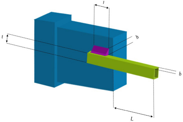
Welded Beam Design.
The results stemming from the application of the proposed IMPA are diligently compared with those obtained through other established methods. The outcomes are meticulously detailed in Table 9, providing optimal parameter values and objective function values for all the algorithms under comparative scrutiny. Remarkably, the IMPA stands out as a paragon of reliability, outperforming other state-of-the-art methodologies. It yields optimal variables represented as h = 2.42253E−01, l = 6.15443E+00, t = 8.54323E+00, b = 2.64534E−01, accompanied by the best objective function value f(x) = 1.69524E+00. The overall average are also superior to other algorithms, indicating that the IMPA algorithm proposed in this paper exhibits excellent optimization ability and stability for the design problem.
Table 9.
Comparison results for Welded Beam Design.
| Algorithm | h | l | t | b | f(x) |
|---|---|---|---|---|---|
| RIME | 2.23490E−01 | 6.23300E+00 | 8.43230E+00 | 2.43215E−−01 | 5.57000E+08 |
| AVOA | 2.43500E−01 | 6.32400E+00 | 8.43220E+00 | 2.54344E−01 | 1.79000E+00 |
| GTO | 2.54343E−01 | 6.54342E+00 | 8.54353E+00 | 2.43252E−01 | 1.05093E+05 |
| OMA | 3.14332E−01 | 7.43252E+00 | 8.13230E+00 | 2.23445E−01 | 3.30139E+17 |
| IWSCA | 2.48900E−01 | 6.17320E+00 | 8.51220E+00 | 3.21215E−01 | 3.12110E+00 |
| MPA | 2.54300E−01 | 7.32300E+00 | 9.13800E+00 | 2.54315E−01 | 1.70000E+00 |
| EMPA | 2.34520E−01 | 6.53300E+00 | 7.13200E+00 | 2.25315E−01 | 3.89153E+00 |
| GDMPA | 2.43250E−01 | 6.34300E+00 | 8.54432E+00 | 2.54323E−01 | 4.44063E+00 |
| IMPA | 2.42253E−01 | 6.15443E+00 | 8.54323E+00 | 2.64534E−01 | 1.69524E+00 |
For a visual insight into the effectiveness of the IMPA, the objective function is presented in Fig. 8. This graphical representations aptly showcase the IMPA's ability to swiftly converge towards the optimal solution within 15 iterations. The parameter values and parameter's curve further substantiate the algorithm's efficacy. It is abundantly clear that the recommended IMPA has delivered outstanding results, yielding optimal parameters and objective function values that contribute significantly to the problem's resolution.
Figure 8.
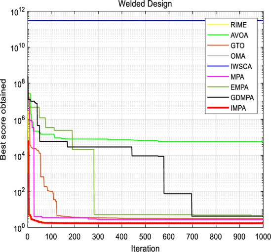
Convergence curves for Welded Beam Design.
Tension/compression spring design
The primary objective of this study revolves around the reduction of total weight in a specific spring design problem35. The fundamental of this tension/compression spring design issue lies in the quest to minimize the overall weight of the designated spring. This endeavor necessitates the modulation of three key variables, namely wire diameter (d), mean coil diameter (D), and the number of active coils (N), as visually portrayed in Fig. 9. The mathematical model of tension/compression spring design is described as follows:
Figure 9.
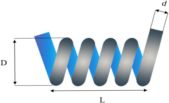
Tension/Compression Spring Design.
The IMPA performance is assessed in comparison to other established methods. Table 10 presents the results and optimal parameter values, encompassing the best outcomes for all comparative techniques, including the proposed IMPA. Remarkably, the IMPA showcases superior performance, furnishing a more robust solution with optimal variable values at d = 5.17750E−02, D = 3.58791E−01, N = 1.11683E+01, and the best objective value of f(x) = 3.63877E+00. The overall average are also superior to other algorithms, indicating that the IMPA algorithm proposed in this paper exhibits excellent optimization ability and stability for the design problem.
Table 10.
Comparison results for Tension/Compression Spring Design.
| Algorithm | d | D | N | f(x) |
|---|---|---|---|---|
| RIME | 5.16788E−02 | 3.56874E−01 | 1.12568E+01 | 4.78000E+02 |
| AVOA | 5.19874E−02 | 3.68742E−01 | 1.35488E+01 | 5.15000E+01 |
| GTO | 5.25468E−02 | 3.65440E−01 | 1.23154E+01 | 5.18679E+01 |
| OMA | 5.18798E−02 | 3.87890E−01 | 1.45475E+01 | 1.53519E+04 |
| IWSCA | 5.18698E−02 | 3.35409E−01 | 1.36897E+01 | 4.44719E+01 |
| MPA | 5.16430E−02 | 3.36300E−01 | 1.13959E+01 | 3.64000E+00 |
| EMPA | 5.19432E−02 | 3.39781E−01 | 1.68896E+01 | 6.64441E+01 |
| GDMPA | 5.18868E−02 | 3.43530E−01 | 1.58759E+01 | 4.92905E+01 |
| IMPA | 5.17750E−02 | 3.58791E−01 | 1.11683E+01 | 3.63877E+00 |
The objective cost curves of the proposed IMPA, which are presented in Fig. 10. This graphical representations offer a compelling illustration of the IMPA's ability to swiftly converge towards the optimal solution within the first 20 iterations. The curves of the parameter values further underscore the efficacy of the IMPA.
Figure 10.
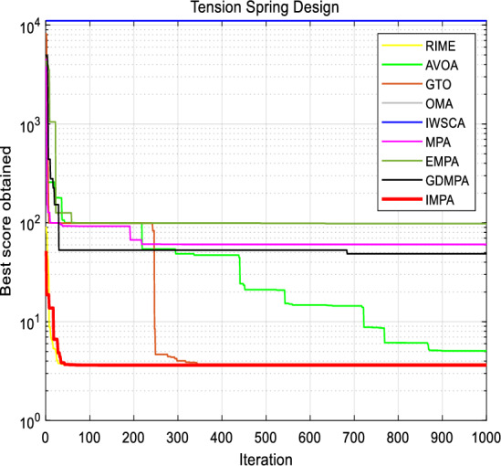
Convergence curves for Tension Spring Design.
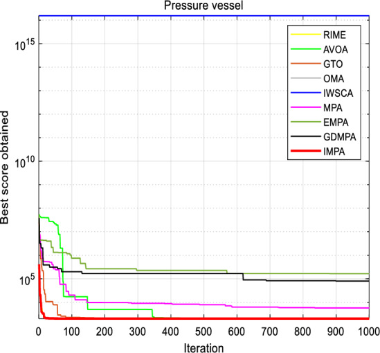
Pressure vessel design
The primary aim of this engineering challenge is to minimize the weight of a specific type of cylindrical pressure vessel36. This study centers its examination on four key design parameters, which include the shell width (x1), head width (x2), internal radius (x3), and the height of the cylindrical part, excluding the head (x4), as thoughtfully illustrated in Fig. 11. The mathematical model of pressure vessel design is described as follows:
Figure 11.
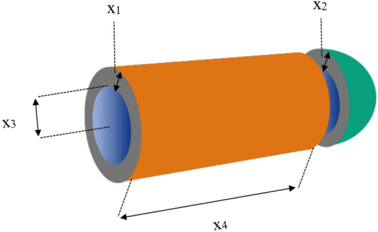
Pressure Vessel Design.
IMPA's results are meticulously assessed and juxtaposed with those obtained through other well-established techniques. A comprehensive presentation of the results is encapsulated in Table 11, featuring optimal parameter values achieved by each algorithm. The proposed IMPA emerges as a beacon of reliability, yielding optimal parameters represented as x1 = 8.125000E−01, x2 = 4.37500E−01, x3 = 4.209840E+01 and x4 = 1.76638E+03, along with the best objective value f(x) = 2.49878E+03. The overall average are also superior to other algorithms, indicating that the IMPA algorithm proposed in this paper exhibits excellent optimization ability and stability for the design problem.
Table 11.
Comparison results for Pressure Vessel Design.
| Algorithm | x1 | x2 | x3 | x4 | f(x) |
|---|---|---|---|---|---|
| RIME | 8.125000E−01 | 4.37500E−01 | 4.204861E+01 | 1.77707E+03 | 3.13000E+03 |
| AVOA | 8.250000E−01 | 6.25000E−01 | 5.598700E+01 | 1.84454E+03 | 2.50000E+03 |
| GTO | 9.375000E−01 | 4.37500E−01 | 4.209130E+01 | 1.76746E+03 | 2.49899E+03 |
| OMA | 8.125000E−01 | 4.34500E−01 | 4.032390E+01 | 1.12679E+03 | 9.29135E+08 |
| IWSCA | 9.375000E−01 | 5.00000E−01 | 4.832900E+01 | 1.17711E+03 | 2.56228E+03 |
| MPA | 8.125000E−01 | 4.37500E−01 | 4.206500E+01 | 1.80823E+03 | 2.50000E+03 |
| EMPA | 8.125000E−01 | 4.12500E−01 | 4.209130E+01 | 1.76746E+03 | 2.57532E+03 |
| GDMPA | 7.975000E−01 | 5.22000E−01 | 4.132390E+01 | 1.52123E+03 | 2.59322E+03 |
| IMPA | 8.125000E−01 | 4.37500E−01 | 4.209840E+01 | 1.76638E+03 | 2.49878E+03 |
To substantiate the algorithm's efficacy, the objective cost curves is presented in Fig. 12. These visual representations aptly demonstrate that the IMPA swiftly converged to the optimal solution before reaching the 30th iteration. The figures displaying parameter values and the curve further reinforce the algorithm's effectiveness in addressing the pressure vessel design problem.
Figure 12.
Convergence curves for Pressure Vessel Design.
Three bar design
This question is intended to minimize the weight of a particular three shot Truss37. The two main design parameters studied in this issue are the cross-sectional area of component 1 (x1), component 2 (x2) and component 3 (x3), as shown in Fig. 12. Use the proposed IMPA to obtain the optimal solution and compare the results with other established methods. The mathematical model of the Three-bar truss design problem is mathematically described as follows:
Table 12 summarizes the results of the competitive approach in solving the three link Truss design problem, including the recommended IMPA. This table provides the optimal parameter values obtained by all algorithms. It is evident that the proposed IMPA produces more reliable results than other state-of-the-art methods. The optimal solution obtained by IMPA is x1 = 7.886654E−01 and x2 = 4.082758E−01, with the optimal objective function value f(x) = 1.863895E+02. The overall average are also superior to other algorithms, indicating that the IMPA algorithm proposed in this paper exhibits excellent optimization ability and stability for the design problem.
Table 12.
Comparison results for Three Bar Truss Design.
| Algorithm | x1 | x2 | f(x) |
|---|---|---|---|
| RIME | 7.88249E−01 | 4.07589E−01 | 2.69000E+03 |
| AVOA | 7.87588E−01 | 4.15789E−01 | 1.87000E+02 |
| GTO | 7.85787E−01 | 4.12234E−01 | 1.92644E+02 |
| OMA | 7.97575E−01 | 4.09634E−01 | 5.64050E+03 |
| IWSCA | 7.96758E−01 | 4.09638E−01 | 1.86949E+02 |
| MPA | 7.88649E−01 | 4.08234E−01 | 1.86000E+02 |
| EMPA | 7.33575E−01 | 4.09834E−01 | 1.86719E+02 |
| GDMPA | 7.86685E−01 | 4.09634E−01 | 1.86442E+02 |
| IMPA | 7.88665E−01 | 4.08275E−01 | 1.86389E+02 |
Figure 13 shows the convergence curve of the objective function of the proposed IMPA. The IMPA can quickly find the optimal solution, which can be achieved with only 15 iterations, as shown in the convergence diagram in Fig. 14. The first parameter curve aim to demonstrate the effectiveness of the proposed IMPA. The convergence curve indicates that the IMPA provides excellent results and quickly provides an ideal solution. In addition, the diversity of potential solutions has been confirmed.
Figure 13.

Three Bar Truss Design.
Figure 14.
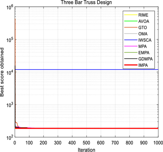
Convergence curves for Three Bar Truss.
Conclusion
In summary, the IMPA is a novel optimization algorithm for solving industrial engineering design problems. The IMPA is an innovative approach to the Marine Predators Algorithm by incorporating dynamic social strategy and self-adaptive weight setting, which can relatively quickly find near-optimal solutions and overcome the limitations by avoiding local optima and improving overall performance. The IMPA contributes to the balance of exploration and exploitation through dynamic social strategy and self-adaptive weight. The superiority of IMPA in CEC 2021 functions has been demonstrated. Meanwhile the results of this study demonstrate the effectiveness of the IMPA in finding high-quality solutions for industrial engineering design problems. Compared with optimization methods and other versions of MPA, including versions of MPA, EMPA, GDMPA, RIME, AVOA, GTO, OMA, IWSCA, the IMPA has several advantages and faster convergence to the optimal solution and reduced chances of falling into local minima. Box-plot analyses prove that the IMPA has better accuracy and convergence than other algorithms. Wilcoxon rank tests which performed the method also show that IMPA differs significantly from any other algorithm. The IMPA has also been proven to be more effective in finding high-quality solutions in a shorter period of time. In order to provide a promising solution for industrial engineering design problems and highlight the potential of the IMPA as a useful tool for solving real-world problems. This study has implemented four highly representative engineering design problems, including Welded Beam Design, Tension/Compression Spring Design, Pressure Vessel Design, and Three Bar Design. The experimental results also proved its efficiency in successfully solving complex industrial engineering design problems.
Every method has advantages and disadvantages, and the IMPA is no exception. The improved algorithm may be performed worse than the GTO and OMA for IEEE CEC2021. Therefore in further investigation, we may combine all chaos mapping in the same algorithm and use some adaptive strategies to decide which parameters will be activated. Future research should focus on implementing IMPA on multi-objective optimization. This would allow for more extensive testing of the algorithm's capabilities and provide a better understanding of its potential in real-world applications.
Acknowledgements
The authors are grateful to Jiangsu vocational college of information technology for a partial financial sponsorship and their facility support in this research.
Author contributions
Conceptualization: Y.C. Data curation: Y.C. Formal analysis: X.H. Investigation: Y.C., X.H. Methodology: Y.C.. Project administration: X.H. Software: Y.X.Y. Supervision: X.H. Validation: C.Q. Writing – original draft: YC.
Funding
This research was funded by National Natural Science Foundation of China (62106088), High-level Professional Group Construction Project of Higher Vocational Education in Jiangsu Province (SJZH [2021] No. 1) , Excellent Science and Technology Innovation Team of Colleges and Universities in Jiangsu Province (SJK [2023] No. 3) and Jiangsu vocational college of information technology Research Funding Project (JSITKY202305).
Data availability
Data used in this study are available upon reasonable request to the corresponding author.
Competing interests
The authors declare no competing interests.
Footnotes
Publisher's note
Springer Nature remains neutral with regard to jurisdictional claims in published maps and institutional affiliations.
References
- 1.Zervoudakis, K. & Tsafarakis, S. A mayfly optimization algorithm. Comput. Ind. Eng.145, 106559. 10.1016/j.cie.2020.106559 (2020). [Google Scholar]
- 2.Mohammadi-Balani, A., Dehghan Nayeri, M., Azar, A. & Taghizadeh-Yazdi, M. Golden eagle optimizer: A nature-inspired metaheuristic algorithm. Comput. Ind. Eng.152, 107050. 10.1016/j.cie.2020.107050 (2021). [Google Scholar]
- 3.Yuan, Y. L., Shen, Q. L. & Wang, S. Coronavirus mask protection algorithm: A new bio-inspired optimization algorithm and its applications. J. Bionic Eng.20, 1. 10.1007/s42235-023-00359-5 (2023). [DOI] [PMC free article] [PubMed] [Google Scholar]
- 4.Kaveh, A. & Dadras Eslamlou, A. Water strider algorithm: A new metaheuristic and applications. Structures25, 520–541. 10.1016/j.istruc.2020.03.033 (2020). [Google Scholar]
- 5.Chou, J.-S. & Truong, D.-N. Multiobjective optimization inspired by behavior of jellyfish for solving structural design problems. Chaos Solitons Fract.135, 109738. 10.1016/j.chaos.2020.109738 (2020). [Google Scholar]
- 6.Yuan, Y. L. et al. Learning-imitation strategy-assisted alpine skiing optimization for the boom of offshore drilling platform. Ocean Eng.1, 114317. 10.1016/j.oceaneng.2023.114317 (2023). [Google Scholar]
- 7.Yuan, Y. L., Ren, J. J., Shen, Q. L., Wang, S. & Wang, Z. X. Alpine skiing optimization: A new bio-inspired optimization algorithm. Adv. Eng. Softw.2022, 103158. 10.1016/j.advengsoft.2022.103158 (2022). [Google Scholar]
- 8.Mirjalili, S. & Lewis, A. The Marine Predator Algorithm. Adv. Eng. Softw.95, 51–67. 10.1016/j.eswa.2021.115936 (2016). [Google Scholar]
- 9.Abdel-Basset, M., El-Shahat, D., Chakrabortty, R. K. & Ryan, M. Parameter estimation of photovoltaic models using an improved marine predators algorithm. Energy Convers. Manag.227, 113491. 10.1016/j.enconman.2020.113491 (2021). [Google Scholar]
- 10.Shaheen, A. M., Elsayed, A. M., Ginidi, A. R. & EL-Sehiemy, R. A., Alharthi, M. M., & Ghoneim, S. S. M.,. A novel improved marine predators algorithm for combined heat and power economic dispatch problem. Alexandria Engineering Journal61(3), 1834–1851. 10.1016/j.aej.2021.07.001 (2022). [Google Scholar]
- 11.Yu, G., Meng, Z., Ma, H. & Liu, L. An adaptive Marine Predators Algorithm for optimizing a hybrid PV/DG/Battery System for a remote area in China. Energy Rep.7, 398–412. 10.1016/j.egyr.2021.01.005 (2021). [Google Scholar]
- 12.Sylvère Mugemanyi, Z. Q. Marine predators algorithm: A comprehensive review. Mach. Learn. Appl.12, 100471. 10.1016/j.mlwa.2023.100471 (2023). [Google Scholar]
- 13.Mezura-Montes, E. & Coello, C. A. C. An empirical study about the usefulness of evolution strategies to solve constrained optimization problems. Int. J. Gen. Syst.37(4), 443–473. 10.1016/j.measurement.2021.109116 (2008). [Google Scholar]
- 14.Houssein, E. H., Hassaballah, M., Ibrahim, I. E., AbdElminaam, D. S. & Wazery, Y. M. An automatic arrhythmia classification model based on improved Marine Predators Algorithm and Convolutions Neural Networks. Expert Syst. Appl.187, 115936. 10.1016/j.eswa.2021.115936 (2022). [Google Scholar]
- 15.Xinming, Z., & Lin, Q. Three-learning strategy particle swarm algorithm for global optimization problems. Inf. Sci.593, 289–313. 10.1016/j.ins.2022.01.075 (2022). [Google Scholar]
- 16.Yuan, Y. L., Mu, X. K., Shao, X. Y., Ren, J. J. & Zhao, Y. Optimization of an auto drum fashioned brake using the elite opposition-based learning and chaotic k-best gravitational search strategy based grey wolf optimizer algorithm. Appl. Soft Comput.1, 108947. 10.1016/j.asoc.2022.108947 (2022). [Google Scholar]
- 17.Aydemir, S. B. Enhanced marine predator algorithm for global optimization and engineering design problems. Adv. Eng. Softw.84, 103517. 10.1016/j.advengsoft.2023.103517 (2023). [Google Scholar]
- 18.Du, P., Guo, J., Sun, S., Wang, S. & Wu, J. Multi-step metal prices forecasting based on a data preprocessing method and an optimized extreme learning machine by marine predators algorithm. Resourc. Policy74, 102335. 10.1016/j.resourpol.2021.102335 (2021). [Google Scholar]
- 19.Han, B., Li, B. & Qin, C. A novel hybrid particle swarm optimization with marine predators. Swarm Evol. Comput.83, 101375. 10.1016/j.swevo.2023.101375 (2023). [Google Scholar]
- 20.Kumar, S. et al. Chaotic marine predators algorithm for global optimization of real-world engineering problems. Knowl.-Based Syst.261, 110192. 10.1016/j.knosys.2022.110192 (2023). [Google Scholar]
- 21.Chen, J., Luo, F., Li, G. & Wang, Z. Batch Bayesian optimization with adaptive batch acquisition functions via multi-objective optimization. Swarm Evol. Comput.79, 101293. 10.1016/j.swevo.2023.101293 (2023). [Google Scholar]
- 22.Ogunsanya, M., Isichei, J. & Desai, S. Grid search hyperparameter tuning in additive manufacturing processes. Manuf. Lett.35, 102454. 10.1016/j.mfglet.2023.102454 (2023). [Google Scholar]
- 23.Azzini, I. & Rosati, R. A function dataset for benchmarking in sensitivity analysis. Data in Brief42, 108071. 10.1016/j.dib.2022.108071 (2022). [DOI] [PMC free article] [PubMed] [Google Scholar]
- 24.Hassan, A. S. & Othma, E. S. Optimal integration of distributed generation resources in active distribution networks for techno-economic benefits. Energy Rep.6, 3462–3471 (2020). [Google Scholar]
- 25.Su, H., Zhao, D. & Heidari, A. A. RIME: A physics-based optimization. Neurocomputing532, 1. 10.1016/j.neucom.2023.02.010 (2023). [Google Scholar]
- 26.Abdollahzadeh, B., Gharehchopogh, F. S. & Mirjalili, S. African vultures optimization algorithm: A new nature-inspired metaheuristic algorithm for global optimization problems. Comput. Ind. Eng.158, 107408. 10.1016/j.cie.2021.107408 (2021). [Google Scholar]
- 27.Shaheen, A. M., Ginidi, A. R., El-Sehiemy, R. A., El-Fergany, A. & Elsayed, A. M. Optimal parameters extraction of photovoltaic triple diode model using an enhanced artificial gorilla troops optimizer. Energy283, 129034. 10.1016/j.energy.2023.129034 (2023). [Google Scholar]
- 28.Cheng, M.-Y. Moh Nur Sholeh, Optical microscope algorithm: A new metaheuristic inspired by microscope magnification for solving engineering optimization problems. Knowl.-Based Syst.279, 110939. 10.1016/j.knosys.2023.110939 (2023). [Google Scholar]
- 29.Chun, Y., & Hua, Y. Improved sine cosine algorithm for optimization problems based on self-adaptive weight and social strategy. IEEE Access11, 73053–73061. 10.1109/ACCESS.2023.3294993 (2023). [Google Scholar]
- 30.Fu, Q. & Li, Q. An improved multi-objective marine predator algorithm for gene selection in classification of cancer microarray data. Computers in Biology and Medicine160, 107020. 10.1016/j.compbiomed.2023.107020 (2023). [DOI] [PubMed] [Google Scholar]
- 31.Han, M. & Du, Z. Golden-Sine dynamic marine predator algorithm for addressing engineering design optimization. Expert Syst. Appl.210, 118372. 10.1016/j.eswa.2022.118372 (2022). [Google Scholar]
- 32.Rizk-Allah, R. M. An improved sine–cosine algorithm based on orthogonal parallel information for global optimization. Soft Comput.23, 7135–7161. 10.1016/j.eswa.2017.07.043 (2017). [Google Scholar]
- 33.Rizk-Allah, R. M. Hybridizing sine cosine algorithm with multi-orthogonal search strategy for engineering design problems. J. Comput. Design Eng.5(2), 249–273. 10.1016/j.neucom.2022.05.006 (2022). [Google Scholar]
- 34.Huang, F., Wang, L. & He, Q. An effective co-evolutionary differential evolution for constrained optimization. Appl. Math. Comput.186(1), 340–356. 10.1016/j.amc.2006.07.105 (2007). [Google Scholar]
- 35.Mezura-Montes, E. & Coello, C. A. C. An empirical study about the usefulness of evolution strategies to solve constrained optimization problems. Int. J. Gen. Syst.37(4), 443–473 (2008). [Google Scholar]
- 36.Tao, R., Meng, Z. & Zhou, H. A self-adaptive strategy based firefly algorithm for constrained engineering design problems. Apply Soft Comput.107, 107417. 10.1016/j.asoc.2021.107417 (2021). [Google Scholar]
- 37.Qimen, M. E., Garip, Z. & Boz, A. F. Comparison of metaheuristic optimization algorithms with a new modified edeb feasibility constraint handling technique. Electro Eng. Comput. Sci.29(7), 3270–3289. 10.1016/j.eecs.2021.109682 (2021). [Google Scholar]
Associated Data
This section collects any data citations, data availability statements, or supplementary materials included in this article.
Data Availability Statement
Data used in this study are available upon reasonable request to the corresponding author.