

Abstract
Post-hoc comparison procedures are commonly used to determine which group means differ after a significant analysis of variance (ANOVA). Several post-hoc tests have been proposed, but their use requires certain assumptions to be met, such as normality, equality of variance, and balanced group size. This review examined the statistical literature on post-hoc tests and their use in the environmental and biological sciences. Through this review, we found that post-hoc tests are effective but often inadequately used in these sciences. We conducted a search of reputed search engines to identify articles in which post-hoc tests were used and found ten post-hoc tests used in the environmental and biological literature. Tukey HSD (30.04%), Duncan's (25.41%) and Fisher's LSD (18.15%) were the most commonly used post-hoc tests over the past 20 years, whereas the Games-Howell (1.13%), Holm-Bonferroni (1.25%), and Scheffe's tests (2.25%) were the least used. The choice of post-hoc test depended on the statistical method used prior. In addition, the assumptions of applying post-hoc tests were not always verified. In fact, the normality condition was mostly only checked in the cases of Tukey HSD, Duncan's, and Fischer's LSD tests, and equality of variance was often met for the Tukey HSD, Duncan's, Fischer's LSD, and Bonferroni tests. This review opens a new avenue for comparing post-hoc test performance in ANOVA using linear or generalised mixed effect models.
Keywords: Multiple comparison tests, Review, Assumptions, Effective use
0. Introduction
Experimentation is a scientific tool that is widely used to explain phenomena based on the principle of causality under defined and controlled conditions. The analysis of experimental data often includes a comparison of trends in measurements across groups [1]. If the number of groups to be compared is equal to two, a Student's t-test is appropriate when the model residuals follow a normal distribution; otherwise, its non-parametric equivalent is used. However, when the number of groups to be compared is greater than two and the required conditions hold, an analysis of variance (ANOVA) is adopted. In the case of significant differences (null hypothesis rejected), further analysis (post-hoc test) is necessary to identify subgroups that are significantly different from each other [1]. Post-hoc tests, or multiple mean comparison tests, are also used after several other statistical methods, such as the linear mixed effect model (LMEM), generalised linear model (GLM), and generalised least squares model (GLS). Several post-hoc tests that compare more than two groups are found in the behavioural science literature [1], as well as in the applied and biological sciences. The application of these tests requires compliance with certain conditions. For instance, the choice of a post-hoc test is conditioned on certain assumptions [2]. Normality, equality of variance, parity in the number of groups compared, and whether observations are planned or unplanned from one group to another [2] are common conditions. Similarly, there are special post-hoc tests for non-parametric methods.
In practice, these tests are often arbitrarily applied in biological science [1]. However, the examination of these methods (theoretical framework and foundations) including their optimal use has been the subject of many scientific studies [2], [3] in several fields, including agronomy [4], [5]; animal production and veterinary science [6], [7], [8]; medicine [9], [10]; entomology [11], [12]; plant and pathology [13]; and psychology [14]. Day and Quinn [2] revealed that the Student-Newman-Keuls (SNK) and Duncan's tests are the most widely used post-hoc tests, although [15], [16], [17], [18] have criticized the use of these tests. Indeed, Einot and Gabriel [18] introduced a modified Newman-Keuls multiple comparison procedure that reduces the chance of a rejection region and prevents the probability of false rejection due to exceeding the level α using the original test.
Most of these authors concluded that post-hoc tests are designed for different purposes and that there is a more appropriate method for a given type of experimental setup. They barely touched upon which method works in case of non-compliance with application conditions, such as normality of a residual model and equality of residual variance. Also, these studies did not explain which method would be more appropriate in cases of equality or inequality in the number of groups and the performance of methods regarding groups size. However, equality or inequality in the number of groups and heteroscedasticity in terms of parametric [19] and non-parametric tests [20] have been worked on in the literature. Day and Quinn [2] addressed these aspects in the field of ecology. The objective of this article is to present a statistical literature (systematic) review of tests to compare groups after ANOVA and their use in environmental and biological sciences.
1. Methods
1.1. Data sources and search strategy
Research in which post-hoc tests were used, was identified using 4 electronic databases: Science Direct (www.sciencedirect.com), Google Scholar (www.scholar.google.fr), African Journals Online (www.ajol.info), MDPI (https://www.mdpi.com/), and Taylor and Francis (https://www.tandfonline.com/). ScienceDirect, Google Scholar, MDPI, and Taylor and Francis are international databases, while African Journals Online is an Africa-wide database. The search terms included post-hoc tests, multiple comparisons, structuring of means, and differences between means.
1.2. Eligibility criteria and study selection
During our research, we thoroughly examined various search engines that deal with biological or environmental concepts, such as soil sciences and plant nutrition, psychology, criminology, electricity, sport, genetics, agriculture, demography, economics, ecology, epidemiology, breeding (animal and plant), health, nutrition, and food security. We focused on articles published between 2000 and 2020 and saved those that mentioned the use of post-hoc tests. Once uploaded, articles were saved if they mentioned the use of post-hoc tests.
1.3. Data extraction process
We recorded several details from the downloaded papers, such as the name of the journal, title of the paper, authors, continent, country, years, domain, type of review, impact factor, statistical methods, normality, variance equality, types of post-hoc test, number of groups, equal or unequal group size, and software used. We then identified the most-represented domains based on the relative frequency of citations and retained the domains with a frequency of at least 5%. The remaining domains were grouped as other domains.
1.4. Data analysis
The statistical analyses were performed using R (Team, 2020), with a significance level of 5%. The frequency of citations was calculated, and figures were generated using the ggplot2 package [21]. These figures were used to describe the use of post-hoc tests across different domains, as well as in general. We used the Chi-square test to explore the relationship between the use of post-hoc tests and group size (equal or unequal). Additionally, we used a correspondence analysis in the FactoMineR package [22] to understand which post-hoc tests were used after specific statistical methods and which tests were predominant in specific domains. To assess the relationship between post-hoc tests and the normality and homogeneity of variance checking, we used binomial logistic regression. Additionally, bar plots were generated to display the percentage of studies where the required assumptions of ANOVA were checked before using specific post-hoc tests.
2. Results
2.1. Search results and included studies
A systematic literature search was conducted, yielding 13,742 records initially. After removing duplicates, 9,616 records were retained and screened for eligibility based on title, abstract, and keywords. A total of 7,627 records were excluded because they did not meet the review eligibility criteria, and 1,076 records were not related to biology or environmental sciences. The screening process resulted in 913 eligible studies (Fig. 1) across various areas such as genetics, agriculture, biotechnology, breeding and animal health, ecology, medicine, dentistry, nutrition and food security, soil science, plant nutrition, and sports. A range of post-hoc tests were used in the selected studies, including Fisher's Least Significant Difference (LSD) test, Student-Newman-Keuls (SNK) test, Tukey's HSD, Scheffe's test, Duncan's test, Dunnett test, Bonferroni method, Dunn's test, Sidak method, Games-Howell test, and Holm-Bonferroni method. The following section presents a complete description of some of these post-hoc tests.
Figure 1.

Study identification.
2.2. Post-hoc comparison methods
In multiple comparison tests, controlling the α level of significance is insufficient to limit the type I error rate when testing the overall null hypothesis at that level. This is due to the problem of multiplicity, which requires a familywise error rate (FWER) or a per-comparison significance level. When the final conclusion relies on only one p-value, conventional p-values can be compared with the nominal significance level α as a threshold. However, when dealing with multiple testing, it is necessary to use procedures that determine the appropriate rejection regions, per-comparison significance levels, or p-value adjustments. The objective of these procedures is to ensure that the familywise error rate is controlled at α. In this section, we describe some of these procedures, including their formulas and reference sources, as well as their limitations and advantages.
Fisher's Least Significant Difference (LSD) test: Fisher's LSD test, introduced in [23], was one of the first multiple comparison procedures. It is essentially a series of multiple t-tests that use a pooled standard deviation across all groups. The test sets the Type I error rate at a per-comparison level of α, which provides high power, as noted in [2]. The statistical tables for the test were computed by Fisher and Yates, as described in [24].
LSD allows for a direct comparison of two means from two different groups by calculating the smallest significance as if a test had been run on those two means. Any difference greater than the LSD is considered statistically significant. To compute the LSD statistic for comparing group A vs B means, one can use the following formula [25] for a given significance level α (1):
| (1) |
where t= is the critical value from the t-distribution table, is the mean square error obtained from the results of the ANOVA test, and n= is the number of scores used to calculate the means.
LSD is usually performed after the significance of the omnibus ANOVA test and under the condition of equal or unequal group sizes and homogeneity of variance. As a multiple t-test (k tests) on the same data, LSD does not control for family-wise type I error, which is .
Student-Newman-Keuls (SNK): Wrong conclusions due to multiple uses of the t-test led the authors to attempt to abolish the t-test. In this way, [26] presented a new approach using an approximation of the F-test into a range test with the Fisher tables. This test name is derived from the three authors: [27], [28], and [26], who used the first known Studentized Range test, which is a sequential (step-down) procedure for comparison. The Student-Newman-Keuls procedure uses different critical values to compare pairs of means. Therefore, significant differences are more likely to be found. The q-value is computed using the following formula (2) [26]:
| (2) |
where if sample sizes are equal, and if sample sizes are not equal.
The SNK test does not control the type I error, even when the requirements are satisfied. Einot and Gabriel [29] showed an exception when dealing specifically with three groups. In addition, this test is affected by unequal group sizes and variance heterogeneity when these assumptions are not met [17].
Tukey's HSD: Addressing the issue of controlling the family-wise error, [30] proposed the famous honestly significant difference (HSD) test, also known as the T method, Tukey's A, or Tukey's w method, using the Studentized range with the number of groups instead of number of comparisons, as done in SNK. The Tukey's HSD is appropriate when the researcher wants to perform all pairwise comparisons [31]. The modified procedure for unequal sample sizes was published by [32], although Tukey had also proposed the same modification (for different configurations and not published), which provides acceptable power. Similar to each of the tests above, the critical value for each comparison is the same; therefore, each comparison has the same probability of a type I error. These are called “simultaneous tests”. The HSD test statistic for each pair of means is computed using the following formula (3) [33]:
| (3) |
where is the difference between the pair of means used to calculate this, such that ; MSE is the mean square error; and n is the number of observations in each group or treatment. This test is widely used in science, and [31] described it as “the most frequently cited unpublished paper in the history of statistics”. It is designed for equal variance and group size. Researchers have used it because of its ability to produce the fewest type I errors and to be the least sensitive to assumption violations [17]. In fact, after controlling for type I error, Tukey's HSD provides an average power.
Scheffé test: This method is a simultaneous procedure developed by Scheffé [34] for all contrasts (a linear combination of means). Thus, it considers not only pairwise comparisons as [30] does, but also non-pairwise, orthogonal comparisons. This method is used for all possible comparisons, including pairwise comparisons and contrasts. There is a very large number of ways to compare combinations of means, whereas the number of pairwise comparisons is limited to , where r= the number of possible comparisons to be made and m= the number of treatments (or means) in the experiment. Therefore, Scheffé's method adjusts the type I error rate per comparison to a very low level to maintain the FWER at the chosen level (), and it lies below α when there is only a limited number of possible comparisons. The Scheffé test is the most flexible, but it also has the lowest statistical power compared with Fisher's LSD and Tukey's HSD tests. Scheffé [16] uses the following test statistic (4):
| (4) |
where is the between-sample degrees of freedom, is the f statistic value from ANOVA, and MSE is the mean square error from ANOVA. Similar to Tukey's HSD test, Scheffé's test is less sensitive when the requirements are not met. Its critical value depends on the number of means in the comparison, and the test is too conservative compared to methods like Tukey's HSD [31].
Duncan's test: While pointing out the basic differences between several procedures (Fisher's LSD, SNK, Scheffé, etc.), [35] proposed a new multiple range test considering the features revealed. The new test is a modification of the SNK procedure, combining the power advantages found in previous studies (Duncan 1951, 1952). The test is a multiple-range test, except that it uses protection levels related to the number of means between the means in comparison. Duncan's Multiple Range test (DMRT) was originally designed as a higher-power alternative to Newman–Keuls. It is more useful than LSD when larger pairs of means are compared, especially when those values are in a table that guards against type I errors. The DMRT statistic is computed using the same algorithm as for Fisher's LSD (5). However, instead of looking up the critical value in a t-table, the q-table is used for each comparison.
| (5) |
where t is the critical value from the q-distribution table, MSE is the mean square error obtained from the results of the ANOVA test, and and are the numbers of observations in groups A and B, respectively. Despite its high power, this test provides an increasing type I error rate (even when assumptions hold) for more than three comparisons [17] and is affected by unequal group size [36].
Dunnett test: When we consider comparisons between a treatment group and control group, Tukey's HSD and Scheffe's procedure provide a wider confidence interval, which is not needed. This problem was addressed by [37], who proposed a procedure to compare several treatments with a control. Dunnett's test (also called Dunnett's Method or Dunnett's Multiple Comparison) compares the means from several experimental groups against a control group mean to determine if there is a difference. One fixed “control” group is compared to all the other samples, so it should only be used when there is a control group. As Dunnett's test compares two groups, it acts similarly to a t-test. The following formula is used to compare the mean difference (6) [37]:
| (6) |
where is the critical value in the Dunnett-critical value table, MSE = mean square error, and and are the numbers of observations for the control group and group in comparison, respectively. However, this method was designed using table for only equal group sizes. Otherwise, the test provides just an approximation [37].
Bonferroni method: Dunn [38] developed a method for constructing simultaneous confidence intervals for a selected number of contrasts (not all possible linear contrasts, as Scheffe did) for a given number of means in comparison. The result is a simultaneous test using the Student t distribution and is conservative for a large number of comparisons or when the test statistics are positively correlated [39]. This reduced the power of the test. The Bonferroni method involves adjusting the significance level per comparison, using the Bonferroni inequality (hence the name), to ensure that the FWER is always below the level chosen (). [38] first computed the Bonferroni correction as follows (7):
| (7) |
where is the desired familywise error rate (often .05, but not necessarily) and k is the number of comparisons (statistical tests). If FWER <α, then the method is stricter than what is allowed. Such methods are also referred to as conservative methods. For the Bonferroni method, the conservativeness increases with the number of simultaneous tests (m). This comes from the probability terms that are omitted in the expression of the FWER. Therefore, when m is large, the Bonferroni method is not recommended. Also, it is more sensitive to unequal group size than heteroscedasticity [40].
Dunn's test: Some alternative methods, like Kruskal-Wallis or the Wilcoxon method, are used to detect significant differences among groups, but few such alternative methods have been developed. Dunn [41] found that this test is adequate for hand computation and better for revealing the differences between groups that are close together. This distribution-free test is usually performed after the rejection of a non-parametric group difference test. This is one of the least powerful multiple comparison tests and can be very conservative, especially for larger numbers of comparisons. When comparing groups A and B, [38] used the test statistic (8):
| (8) |
where ; is the total sample size of the k groups; r is the number of tied ranks across all k groups; is the number of observations across all k groups with the s tied rank; and is the per-group average rank with being the group's summed ranks.
The Sidak method:[42] worked on finding a rectangular confidence region for a multivariate normal distribution. A slight modification of the Bonferroni method was proven to be “best” when the variances are known or unknown but equal. [38]. The Sidak method gives a familywise error equal to the nominal level (unlike the Bonferroni method, for which it is below) and results in an increase in power compared to the Bonferroni method. The Sidak method is based on the assumption that all tests are mutually independent under , i.e., all test statistics for the partial null hypotheses are mutually independent under . This is an unrealistic assumption for many applications (e.g., test statistics may share the same sample mean), but it simplifies the expression for FWER (similar to the omission of probability terms in the development of the Bonferroni method). Sidak [42] defined the per-comparison significance level for controlling the FWER at α as follows (9):
| (9) |
It can be shown that the method of Sidak is conservative but less conservative than the Bonferroni method. The latter follows from the fact that . The per-comparison significance level of the Bonferroni method is never higher than that of the Sidak method. Hence, the power of the Sidak procedure is generally greater than that of the Bonferroni procedure.
Games-Howell test: The authors were interested in the robustness of the latter procedures (HSD, LSD, etc.) when conditions are violated [43]. Games and Howell [44] addressed the problem of unequal variances and group sizes while comparing the Tukey-Kramer test, t-test, and their BF test (Behrens-Fisher modification of the Tukey HSD). The proposed BF test incorporates the Welch degree-of-freedom solution and weighted pooled variance instead of MSE. It performs better when the sample sizes and variances are unequal. The Games-Howell procedure controls for type I error per comparison in heterogeneity variances and group sizes compared to the Tukey-Kramer procedure. A comparison of k groups is statistically significant if the following holds (10) [40]:
| (10) |
where and are the means of groups i and j, respectively; is the weighted pooled variance for the two groups; and is the Studentized range value.
This is performed for unequal variance and sample sizes, which is usually the structure of the data. The test can fairly control the type I error rate when the requirements are satisfied. Moreover, the Games-Howell test has more power when the assumptions are violated compared to several post-hoc tests.
Holm-Bonferroni method: The Bonferroni-Holm method, also referred to as the Holm method [45], sequential Bonferroni, or Holm-Bonferroni method, is an alternative approach to counteract the problem of multiple comparisons. Holm [45] proposed a modification of the Bonferroni procedure by using sequential comparison to different levels instead of a constant one. The obtained test is uniformly more powerful than the classical Bonferroni test. Although Bonferroni correction controls the FWER by rejecting null hypotheses with a p-value less than , the cost is an increased risk of accepting the false null hypothesis (type II error). Holm [45] proved that his test maintains the FWER at a specified level in the strong sense. Moreover, the test has a gain of power compared to the classical Bonferroni, especially when the null hypothesis is completely wrong. Holm [45] presented the following steps for executing this procedure:
1. Order the p-values from small to large:
where denotes the -order statistic of the set of m p-values.
2. If , then the partial null hypothesis that corresponds to this p-value is rejected, and the method proceeds (go to step 3). Otherwise, no partial hypotheses are rejected and the procedure stops here.
3. If , then the partial null hypothesis corresponding to this p-value is rejected, and the method proceeds (go to step 4). Otherwise, no further partial hypotheses are rejected and the procedure stops here.
4. For a general , if , then the partial null hypothesis corresponding to this p-value is rejected, and the method proceeds as long as . As soon as , the procedure stops and no further partial hypotheses are rejected.
In other words, for the smallest p-value, the classical Bonferroni method is applied. If this result is significant, the method proceeds to the next smallest p-value, and the method of Bonferroni is used again, but this time on the remaining p-values (thus, the Bonferroni method needs to adjust for only tests and is thus less strict). Each time a significant test result is obtained, the method is allowed to proceed at a larger per-comparison significance level. Hence, this method is more powerful than the classical Bonferroni method. Note that the FWERs of the Bonferroni and Holm-Bonferroni methods coincide because FWER depends only on the smallest adjusted p-value, and these are the same for both methods.
2.3. Use of post-hoc tests in biological and environmental sciences
2.3.1. Current use of post-hoc tests according to the domain
The proportions of effective uses of post-hoc tests in general and per applied field considered are presented in Table 1. Tukey HSD (30.04%), Duncan (25.41%), and Fisher's LSD (18.15%) were the most used post-hoc tests over the past twenty years. In contrast, the Games-Howell test (1.13%), Holm-Bonferroni (1.25%), and Scheffe's test (2.25%) were the least used. In most domains, Tukey HSD was the most commonly used post-hoc test. Apart from Tukey HSD, Duncan's test (20%) and Fisher's LSD (20%) were the most commonly used in genetics. In agriculture, Duncan's test (32.68%) and Fisher's LSD (28.74%) were mostly used. In biotechnology, Duncan's test (40%) was the most used. In breeding and animal health, Duncan's test (33.33%) was the most highly cited test in the literature. In dentistry, Bonferroni (26.41%) and Tukey HSD (54.72%) were the most frequently cited tests. In soil sciences and plant nutrition, the most commonly used post-hoc tests were Duncan (25.40%), Fisher's LSD (26.98%), and Tukey HSD (34.92%). In ecology, Tukey HSD (51.61%) and Fisher's LSD (19.36%) were the most cited. In medicine, the Bonferroni procedure (22.39%) and Tukey HSD (20.90%) were mainly used, while in nutrition and food security, Duncan's (46.08%) and Tukey HSD (28.70%) were used. Furthermore, the Bonferroni procedure was the most used post-hoc test in sports sciences (50%), followed by Tukey HSD (28.13%).
Table 1.
Row profile of the use of post-hoc tests according to domain (%).
| Effective use | Domains | Bonferroni Procedure | Duncan's test | Dunnett's correction | Dunn's test | Games-Howell test | Holm-Bonferroni | Fisher's LSD | Scheffé's | SNK | Tukey HSD |
|---|---|---|---|---|---|---|---|---|---|---|---|
| Overall use | 9.637 | 25.407 | 4.506 | 4.255 | 1.126 | 1.252 | 18.148 | 2.253 | 3.379 | 30.038 | |
| Research field | Genetics | 6.667 | 20.000 | 0.000 | 0.000 | 0.000 | 0.000 | 20.000 | 0.000 | 0.000 | 53.333 |
| Agriculture | 1.575 | 32.677 | 3.543 | 2.756 | 0.787 | 0.000 | 28.740 | 0.000 | 4.331 | 25.591 | |
| Biotechnology | 0.000 | 40.000 | 0.000 | 0.000 | 10.000 | 0.000 | 15.000 | 0.000 | 5.000 | 30.000 | |
| Breedings and animal health | 7.143 | 33.333 | 4.762 | 9.524 | 0.000 | 4.762 | 11.905 | 2.381 | 4.762 | 21.429 | |
| Dentistry | 26.415 | 0.000 | 5.660 | 7.547 | 1.887 | 1.887 | 1.887 | 0.000 | 0.000 | 54.717 | |
| Ecology | 3.226 | 12.903 | 3.226 | 3.226 | 3.226 | 0.000 | 19.355 | 0.000 | 3.226 | 51.613 | |
| Medicine | 22.388 | 11.940 | 9.701 | 10.448 | 1.493 | 1.493 | 11.194 | 6.716 | 3.731 | 20.896 | |
| Nutrition and food security | 3.478 | 46.087 | 4.348 | 1.739 | 0.870 | 0.000 | 10.435 | 2.609 | 1.739 | 28.696 | |
| Others | 10.000 | 15.000 | 2.500 | 2.500 | 0.000 | 0.000 | 20.000 | 10.000 | 2.500 | 37.500 | |
| Soil science and Plant nutrition | 0.000 | 25.397 | 3.175 | 1.587 | 0.000 | 1.587 | 26.984 | 0.000 | 6.349 | 34.921 | |
| Sport | 50.000 | 0.000 | 0.000 | 0.000 | 0.000 | 12.500 | 6.250 | 3.125 | 0.000 | 28.125 | |
2.3.2. Use of post-hoc tests according to group size (equal or unequal)
The Chi-square independence test showed dependence between the test used and the equality of size of the groups in comparison (DF = 108; Chi2 = 400.78; Prob <0.001). In the case of equality in group size, the most commonly used tests were the Tukey HSD, Duncan, and Fisher's LSD tests. In cases of unequal group size, Tukey HSD, Fisher's LSD, Duncan, and Bonferroni were mostly used (Fig. 2).
Figure 2.
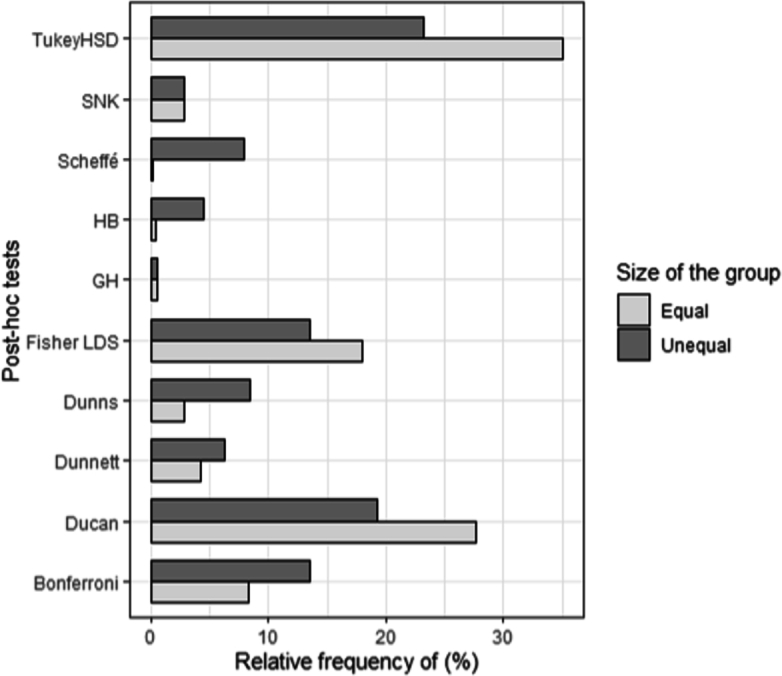
Relative use of post-hoc tests regarding size of groups. Bonferroni : Bonferroni test; Ducan: Duncan test ; Dunnett: Dunnett's test; Dunns : Dunn's test ; GH : Games-Howell test ; HB : Holm-Bonferroni test ; Fischer LSD : Fisher's Least Significant Difference test ; Scheffé : Scheffé's test ;SNK : Newman-Keuls test; Tukey HSD : Tukey Honestly Significant Difference.
2.3.3. Use of post-hoc tests in relation with statistical analysis methods and domains
The choice of post-hoc tests depends on the statistical method used (Chi2 = 479.88, Prob <0.001). From the correspondence analysis, the first two axes consider 83.83% of the variability in the information on the number of uses of post-hoc tests regarding the statistical methods. Duncan's test was the most used after the Kruskal-Wallis test. Duncan, Fisher's LSD, Tukey, SNK, Games-Howell, and Dunnet tests were used after ANOVA, mixed ANOVA, linear mixed effect model, and generalized linear models. Bonferroni and Scheffe's tests were mostly used after the t-test and generalized linear models (Fig. 3).
Figure 3.

Correspondence analysis biplot of post-hoc procedures and statistical methods. Bonf: Bonferroni; Duc:Duncan ; Dun_c: Dunnett's correction ; Dunns : Dunn's test ; GH : Games-Howell ; HB : Holm-Bonferroni ; LSD : Fisher's Least Significant Difference ; Schf : Scheffé ;SNK : Newman-Keuls; Tukey HSD GLM: Generalized Linear Models; Anova: Analysis of variance; LMEM: Linear Mixed Effect Models; t-test: Test t de Student; KW: Kruskal Wallis test; MW: Mann Whitney test.
Fig. 4 presents the relationship between post-hoc procedures and their respective domains of use. The Holm-Bonferroni procedure is widely used in sports and related sciences, while the Bonferroni procedure is more commonly used in dentistry. In Medicine, the most commonly used tests were Dunns, Scheffé, and Dunnett. Fisher's LSD and Tukey HSD were used in several domains.
Figure 4.

Correspondence analysis biplot of post-hoc procedures and domain of use. Genetics: Gene; Agriculture: Agri; Biotechnology: Biotech; Breeding and animal health: BAH; Dentistry: Dent; Ecology: Eco; Medicine: Med; Nutrition and food security: NFS; Others: Others; Soil science and Plant nutrition: SPN; Sport: Sports.
2.4. Post-hoc test effectiveness
Failure to verify normality before choosing post-hoc tests varied significantly depending on the test. Indeed, compared with the Tukey test, the proportion of non-verification of normality in the literature was significantly different among the Bonferroni, Duncan, Dunnett, Dunns and Scheffé tests (Prob <0.05, Table 2). Fig. 5 presents the proportion of articles in which the application conditions of ANOVA were checked for each post-hoc test. The tests for which normality was better verified were Tukey, Dunns, and Fischer's LSD tests (Fig. 5). The proportion of failures to verify the equality of variance before choosing post-hoc tests also varied significantly depending on the test. Compared to the Tukey test, the non-verification of the equality of variance was significant compared to the Bonferroni, Duncan, Dunns, and Scheffé tests (Prob <0.05) (Table 2). The tests for which the equality of variance was verified more were the Tukey, Dunns, Fischer LSD, and Bonferroni tests (Fig. 5). In addition, these conditions of use were most verified in agriculture (Fig. 6).
Table 2.
Normality and equality of variance checking in relation to the post-hoc tests.
| Post-hoc tests and domains | Estimate (se) | z value | Pr(>|z|) |
|---|---|---|---|
| Normality | |||
| Tukey | - | - | - |
| Bonferroni | 1.16 (0.31) | 3.7 | 0.001 |
| Duncan | -1.06 (0.30) | -3.47 | 0.001 |
| Dunnett | 0.81 (0.39) | 2.08 | 0.037 |
| Dunn | 2.94 (0.52) | 5.7 | 0.001 |
| GH | 0.19 (1.17) | 0.17 | 0.868 |
| HB | 0.89 (0.67) | 1.33 | 0.183 |
| LSD | -0.22 (0.27) | -0.8 | 0.424 |
| Scheffé | 2.17 (0.56) | 3.89 | 0.001 |
| SNK | 0.71 (0.43) | 1.65 | 0.101 |
| Equality of variance | |||
| Tukey | - | - | - |
| Bonferroni | 0.69 (0.34) | 2.02 | 0.044 |
| Duncan | -0.92 (0.33) | -2.81 | 0.005 |
| Dunnett | 0.69 (0.42) | 1.66 | 0.097 |
| Dunn | 3.22 (0.52) | 6.17 | 0.001 |
| GH | 0.47 (1.17) | 0.4 | 0.687 |
| HB | 1.16 (0.67) | 1.74 | 0.083 |
| LSD | -0.14 (0.30) | -0.49 | 0.628 |
| Scheffé | 2.45 (0.56) | 4.34 | 0.001 |
| SNK | 0.47 (0.47) | 1 | 0.32 |
GH: Games-Howell; HB: Holm-Bonferroni; LSD: Fisher's Least Significant Difference; SNK: Newman-Keuls
Figure 5.

Proportion of articles in which the application conditions are checked regarding the test. Bonf: Bonferroni; Duc: Duncan; Dun_c: Dunnett's correction; Dun : Dunn's test; GH : Games-Howel; HB : Holm-Bonferroni; LSD : Fisher's Least Significant Difference; Schf : Scheffé; SNK : Newman-Keuls; Tukey HSD.
Figure 6.

Proportion of articles in which the application conditions are checked regarding the domain.
3. Discussion
In this study, we investigated the effective use of post-hoc tests various fields: Agriculture, Biotechnology, Breeding and Animal Health, Ecology, Genetics, Medicine, Nutrition and Food Security, Soil Science and Plant Nutrition, and Sports. The results suggest certain trends, which are discussed in this section.
3.1. Use of post-hoc tests: is there specific use according to different fields?
This study demonstrated that various post-hoc tests were used, with Tukey HSD being the most popular across all fields. However, no direct correlation was found between the choice of tests and the specific fields of study. It is unclear whether users only choose tests with which they are familiar or if they base their choices on the data structure. We can conclude that there is no clear reasoning behind the selection of post-hoc tests by users, but choosing the correct test can lead to valuable insights and interpretations [46]. For instance, Day and Quinn [2] suggested that ecologists consider whether they can frame specific questions to test using orthogonal planned comparisons with a per-comparison error rate. Even if a specific post-hoc test is adequate for a domain, the authors or users must clearly define the procedure used and at least present the test statistics [1]. Authors are used to only giving the p-value and conclusion.
3.2. Holding of post-hoc test assumptions
According to the results, the conditions for applying post-hoc tests, namely, normality and homogeneity of variances, were rarely checked by the authors. This was attributed to the ignorance of users in the applied sciences, who were not always aware of the subtleties of choosing appropriate tests. In addition, users may be limited by the comparison tests available in the statistical software used. However, as discussed by several authors, various methods have been recommended for each situation. Appropriate post-hoc tests are available for both parametric and non-parametric analyses. Non-parametric post-hoc tests include the Dunn, Steel, Nemenyi, and Steel-Dwass tests [2]. For parametric post-hoc tests, there are tests available for both equality and inequality of variance, such as Fisher's LSD, Scheffé, Tukey, Duncan, and Student-Newman-Keuls (SNK) for equal variances and Games-Howell, T'method, and Krammer's for unequal variances [2]. Dunnett's test is a post-hoc test that can be used to compare groups to a benchmark when the variance is equal [2]. Post-hoc tests are also appropriate for comparing groups of equal or unequal size [2]. Recommendations have been made for the selection of relevant post-hoc tests among parametric tests when dealing with some violation conditions [19]. While a normal distribution is required for some post-hoc tests, real data may not meet this criterion; therefore, non-parametric post-hoc tests are strongly recommended. Day and Quinn [2] noticed that, in biology, data are usually log-normal when the variances are unequal. A plot can help determine whether a log transformation can normalize the data. However, if the transformation after plotting residuals or box plots is not useful, non-parametric post-hoc tests are strongly recommended. Recently, Dolgun and Demirham [47] suggested the use of the Steel-Dwass procedure with Holm's approach when the number of groups is small and Dunn's method for a greater number of groups.
3.3. Post-hoc tests use: future directions
Researchers have used various post-hoc procedures, even within the same domain. However, it should be noted that some post-hoc tests are more commonly used in specific domains, despite the fact that no significant association is found between the test and the domain. Moreover, researchers do not provide sufficient justification for choosing a particular post-hoc test. They should explain their selection based on assumptions or the required conditions of use, such as normality and homoscedasticity. For instance, post-hoc tests requiring the normality and homoscedasticity of data could be provided by using positive normality and homoscedasticity tests, respectively. Indeed, more than ten post-hoc tests were found to be used, with different importance of use. Among them, Tukey HSD, Duncan, and Fisher's LSD tests are the most commonly used. These tests are indeed better than others [4], mainly the Tukey test [6] as it protects against type I errors. Moreover, their use does not necessarily require the rejection of the null hypothesis. Fisher's LSD test, in particular, is favoured because of its ease of application and ability to identify even the smallest significant differences [46], [48]. Although Scheffe's test is one of the most recommended tests, it has been used very little over the past two decades [4]. Day and Quinn [2] suggested some post-hoc tests under certain conditions, such as heterogeneity of variances, comparisons of control groups vs. treatment groups, and equal or unequal group sizes. However, a strong study to confirm these suggestions was not conducted during this period. The use of a convenient post-hoc test when the assumptions do not hold was deeply investigated by [19] using various conditions of violation. This wide simulation study compared 18 multiple comparison tests using powers and type I error measures under heterogeneity and dependency conditions. The authors recommended SNK, one of the most powerful tests, in cases of high heterogeneity and a large number of groups for comparison. The same study was conducted by considering non-parametric multiple comparison tests and including a skewed error distribution [47]. Another recent simulation study [40] recommended the Games-Howell procedure when dealing with normal and independent data. Nevertheless, the authors did not study cases violating normality. Further studies could investigate the robustness (performance in terms of power and type I error rate) of several tests when some required assumptions (e.g., heterogeneity of group variances and sizes, residual distributions) do not hold. This will be used as a guideline for researchers performing group difference comparisons. Future studies may focus on the use of post-hoc tests in generalized (mixed) or linear (mixed) models.
4. Conclusion
In this critical review, we examined the use of post-hoc tests to compare means in the environmental and biological sciences. A total of ten post-hoc tests were identified, and their frequency of use varied according to scientific field and period. We found that researchers rarely check post-hoc test assumptions before using or proposing a justification for their choice. This leads to a crucial question: when sample sizes, variances, and normality assumptions are not met, which post-hoc tests can adequately maintain a type I error rate while maintaining strong power? This question is particularly relevant in linear or generalised mixed-effect models and survival analysis, where these conditions are frequently violated. Our critical analysis of the literature highlights the need for an in-depth examination of the use of post-hoc tests, not only in classical ANOVA but also in linear and generalised mixed-effect models and survival analysis. The results of such studies will provide researchers with clear guidelines for performing post-hoc tests.
CRediT authorship contribution statement
Codjo Emile Agbangba: Writing – original draft, Methodology, Formal analysis, Conceptualization. Edmond Sacla Aide: Investigation, Formal analysis, Data curation. Hermann Honfo: Writing – review & editing, Methodology. Romain Glèlè Kakai: Writing – review & editing, Supervision, Conceptualization.
Declaration of Competing Interest
The authors declare the following financial interests/personal relationships which may be considered as potential competing interests:
Codjo Emile Agbangba reports was provided by University of Abomey-Calavi. Codjo Emile AGBANGBA reports a relationship with University of Abomey-Calavi Laboratory of Biomathematics and Forest Estimations that includes: employment. There is no conflict of interest If there are other authors, they declare that they have no known competing financial interests or personal relationships that could have appeared to influence the work reported in this paper.
References
- 1.Ruxton G.D., Beauchamp G. Time for some a priori thinking about post hoc testing. Behav. Ecol. 2008;19(3):690–693. [Google Scholar]
- 2.Day R.W., Quinn G.P. Comparisons of treatments after an analysis of variance in ecology. Ecol. Monogr. 1989;59(4):433–463. [Google Scholar]
- 3.Miller J., Rupert G. Developments in multiple comparisons 1966–1976. J. Am. Stat. Assoc. 1977;72(360a):779–788. [Google Scholar]
- 4.Chew V. Comparing treatment means: a compendium. HortScience. 1976;11:348–357. [Google Scholar]
- 5.Baker R.J. Multiple comparison tests. Can. J. Plant Sci. 1980;60:325–327. [Google Scholar]
- 6.Gill J.L. Current status of multiple comparisons of means in designed experiments. J. Dairy Sci. 1973;56(8):973–977. [Google Scholar]
- 7.Waldo D.R. An evaluation of multiple comparison procedures. J. Anim. Sci. 1976;42(2):539–544. doi: 10.2527/jas1976.422539x. [DOI] [PubMed] [Google Scholar]
- 8.Cox D.F. Design and analysis in nutritional and physiological experimentation. J. Dairy Sci. 1980;63(2):313–321. doi: 10.3168/jds.s0022-0302(80)82932-8. [DOI] [PubMed] [Google Scholar]
- 9.Kusuoka H., Hoffman J.I.E. Advice on statistical analysis for circulation research. Circ. Res. 2002;91(8):662–671. doi: 10.1161/01.res.0000037427.73184.c1. [DOI] [PubMed] [Google Scholar]
- 10.Salsburg D.S. The religion of statistics as practiced in medical journals. Am. Stat. 1985;39(3):220–223. [Google Scholar]
- 11.Jones D. Use, misuse, and role of multiple-comparison procedures in ecological and agricultural entomology. Environ. Entomol. 1984;13(3):635–649. [Google Scholar]
- 12.Perry J.N. Multiple-comparison procedures: a dissenting view. J. Econ. Entomol. 1986;79(5):1149–1155. doi: 10.1093/jee/79.5.1149. [DOI] [PubMed] [Google Scholar]
- 13.Madden J.K.K.L.V., Raymond L. Considerations for the use of multiple comparison procedures in phytopathological investigations. Phytopathology. 1982;72(8):1015. [Google Scholar]
- 14.Jaccard M.B.J., Wood G. Pairwise multiple comparison procedures: a review. Psychol. Bull. 1984;96(3):589. [Google Scholar]
- 15.Ryan T.A. Multiple comparison in psychological research. Psychol. Bull. 1959;56(1):26. doi: 10.1037/h0042478. [DOI] [PubMed] [Google Scholar]
- 16.Scheffe H. John Wiley & Sons; 1999. The Analysis of Variance, vol. 72. [Google Scholar]
- 17.Petrinovich L.F., Hardyck C.D. Error rates for multiple comparison methods: some evidence concerning the frequency of erroneous conclusions. Psychol. Bull. 1969;71(1):43. [Google Scholar]
- 18.Einot I., Ruben G.K. A study of the powers of several methods of multiple comparisons. J. Am. Stat. Assoc. 1975;70(351a):574–583. [Google Scholar]
- 19.Haydar D.Y.P.D., Anil D.N., Ozgur D.M. Performance of some multiple comparison tests under heteroscedasticity and dependency. J. Stat. Comput. Simul. 2010;80:1083–1100. [Google Scholar]
- 20.Anil D., Haydar D. Performance of nonparametric multiple comparison tests under heteroscedasticity, dependency, and skewed error distribution. Commun. Stat., Simul. Comput. 2017;46(7):5166–5183. [Google Scholar]
- 21.Wickham D.N.H., Pedersen T.L. Springer Verlag; New York: 2016. “ggplot2: Elegant Graphics for Data Analysis. [Google Scholar]
- 22.Barranco-Chamorro A.R.-L.I., Muñoz-Armayones S., Romero-Campero F. Smart Data. Chapman and Hall/CRC; 2019. Multivariate projection techniques to reduce dimensionality in large datasets; pp. 133–160. [Google Scholar]
- 23.Fisher R. Oliver and Boyd; 1935. The Design of Experiments. [Google Scholar]
- 24.Fisher R.A., Yates F. Hafner Publishing Company; 1953. Statistical Tables for Biological, Agricultural and Medical Research. [Google Scholar]
- 25.Williams L.J., Hervé A. Fisher's least significant difference (LSD) test. Encycl. Res. Des. 2010;218(4):840–853. [Google Scholar]
- 26.Keuls M. The use of the “studentized range” in connection with an analysis of variance. Euphytica. 1952;1(2):112–122. [Google Scholar]
- 27.Student Errors of routine analysis. Biometrika. 1927;19(1/2):151–164. [Google Scholar]
- 28.Newman D. The distribution of range in samples from a normal population, expressed in terms of an independent estimate of standard deviation. Biometrika. 1939;31:20–30. [Google Scholar]
- 29.Einot I., Gabriel K.R. A study of the powers of several methods of multiple comparisons. J. Am. Stat. Assoc. 1975;70(351a):574–583. [Google Scholar]
- 30.Tukey J.W. Multiple comparisons. 1953. The problem of multiple comparisons. [Google Scholar]
- 31.Toothaker L.E. Sage Publications, Inc.; 1993. Multiple Comparison Procedures. No. 07-089 in Sage University Paper Series on Quantitative Applications in the Social Sciences. [Google Scholar]
- 32.Kramer C.Y. Extension of multiple range tests to group means with unequal numbers of replications. Biometrics. 1956;12(3):307–310. [Google Scholar]
- 33.Hervé A., Williams L.J. Tukey's honestly significant difference (HSD) test. Encycl. Res. Des. 2010;3(1):1–5. [Google Scholar]
- 34.Scheffé H. A method for judging all contrasts in the analysis of variance. Biometrika. 1953;40(1/2):87–104. [Google Scholar]
- 35.Duncan D.B. Multiple range and multiple F tests. Biometrics. 1955;11(1):1–42. [Google Scholar]
- 36.Ozkaya G., Ercan I. Examining multiple comparison procedures according to error rate, power type and false discovery rate. J. Mod. Appl. Stat. Methods. 2012;11(2):7. [Google Scholar]
- 37.Dunnett C.W. A multiple comparison procedure for comparing several treatments with a control. J. Am. Stat. Assoc. 1955;50(272):1096–1121. [Google Scholar]
- 38.Dunn O.J. Multiple comparisons among means. J. Am. Stat. Assoc. 1961;56(293):52–64. [Google Scholar]
- 39.Moran M.D. Arguments for rejecting the sequential Bonferroni in ecological studies. Oikos. 2003;100(2):403–405. [Google Scholar]
- 40.Sauder D. James Madison University; 2017. Examining the type I error and power of 18 common post-hoc comparison tests.https://commons.lib.jmu.edu/cgi/viewcontent.cgi Graduate Psychology. [Google Scholar]
- 41.Dunn O.J. Multiple comparisons using rank sums. Technometrics. 1964;6(3):241–252. [Google Scholar]
- 42.Sidak Z. Rectangular confidence regions for the means of multivariate normal distributions. J. Am. Stat. Assoc. 1967;62(318):626–633. [Google Scholar]
- 43.Ramseyer G.C., Tcheng T. The robustness of the studentized range statistic to violations of the normality and homogeneity of variance assumptions. Am. Educ. Res. J. 1973;10(3):235–240. [Google Scholar]
- 44.Games P.A., Howell J.F. Pairwise multiple comparison procedures with unequal N's and/or variances: a Monte Carlo study. J. Educ. Stat. 1976;1(2):113–125. [Google Scholar]
- 45.Holm S. A simple sequentially rejective multiple test procedure. Scand. J. Stat. 1979;6(2):65–70. [Google Scholar]
- 46.Hulya A., Yakut U. Multiple comparisons. J. Biol. Sci. 2001;1(8):723–727. [Google Scholar]
- 47.Dolgun A., Demirhan H. Performance of nonparametric multiple comparison tests under heteroscedasticity, dependency, and skewed error distribution. Commun. Stat., Simul. Comput. 2017;46(7):5166–5183. [Google Scholar]
- 48.Bek Y., Efe E. vol. 71. Cukurova University; Adana-Turkey: 1995. Experimental Methods. (Course Book of Agricultural Faculty). [Google Scholar]