Multi-objective optimization of laser machining parameters for carbon-glass reinforced hybrid composites: Integrating gray relational analysis, regression, and ANN

Abstract

This research aims to improve the accuracy of cutting fiber-reinforced polymers (FRPs) utilizing CO2 laser processing techniques, with a particular focus on carbon-glass fiber-reinforced hybrid composites (CGFRP) using epoxy resin. Establishing CO₂ laser machining as a dependable and effective process for creating superior CGFRP components is the main goal. This research intends to optimize laser machining parameters to enhance surface quality and machining efficiency for these composites by a thorough parametric analysis. In order to model and improve the correlations between important machining parameters, the research combines regression models, multi-objective gray relational analysis (MOGRA), and Artificial Neural Networks (ANNs). When linked together, these methods enable efficient multi-objective optimization, which enhances laser cutting operations for CGFRP materials in terms of accuracy and economy. Using the Taguchi L27 orthogonal array, one can methodically investigate how different parameters affect CGFRP cutting. GRA is used in optimization to find the best parameter combinations and highlight important parameters. After determining that LPW3CSD1FOL1GPR1 and LPW3CSD2FOL1GPR2 were the ultimate ideal settings, the initial machining parameters were set at LPW3CSD1FOL1GPR1. Predictions and trials confirm that these adjusted parameters result in a 6.125% improvement in grade. Also, ANN structured approach enhances predictive accuracy and provides valuable insights for optimizing machining processes.

Accordingly, a strong framework for enhancing hybrid composite laser machining is provided by this research. The research aims to develop a robust framework for optimizing CO2 laser cutting of CGFRP composites, ultimately leading to more efficient, cost-effective manufacturing solutions for high-performance applications in aerospace, automotive, and marine sectors.

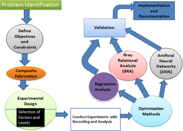
Graphical abstract

Specifications table

Subject area:	Engineering
More specific subject area:	Mechanical Manufacturing
Name of your method:	Gray relational analysis, regression, and ANN
Name and reference of original method:	NA
Resource availability:	NA

Background

Carbon-Glass Fiber Reinforced Polymers (CGFRP) has become indispensable in industries like aerospace, automotive, and marine due to their exceptional strength-to-weight ratio and durability. However, traditional machining methods often encounter challenges such as tool wear and delamination, hindering the achievement of precise cuts.CO2 laser machining presents a compelling alternative, offering a non-contact, precise approach that avoids mechanical stress on the material. The optimization of laser machining processes for composite materials has been a subject of extensive research. Numerous studies have explored the effects of various machining parameters on factors such as cut quality, material removal rate, and overall process efficiency. By systematically varying these parameters and observing their impact on response variables, researchers have developed predictive models that can guide process improvement. For instance [1], successfully employed RSM to identify optimal conditions for laser machining composite materials, leading to enhanced accuracy and productivity. Multi-objective optimization techniques, such as Grey Relational Analysis (GRA), have also been applied to improve the mechanical properties and overall performance of composite materials. [2], demonstrated the effectiveness of GRA in optimizing multiple machining parameters for carbon/glass hybrid composites, resulting in significant enhancements in material characteristics. Studies on CO2 laser cutting of reinforced polyester composites [3] have revealed the optimal parameters for achieving high material removal rates and efficient cutting. High-power fiber lasers have shown promise for cutting thick carbon fiber reinforced polymer (CFRP) laminates in a single pass [4]. Researchers have investigated the effects of laser parameters on cutting quality, surface roughness, and heat-affected zone to identify optimal conditions for this challenging process. Femtosecond laser processing has been explored for its potential to minimize the heat-affected zone (HAZ) in CFRP materials [5]. By optimizing laser parameters, researchers have demonstrated significant reductions in HAZ while preserving material integrity. Multi-objective optimization techniques have also been applied to optimize multiple cutting quality attributes for composite materials, such as kerf width, surface roughness, and heat-affected zone [6].

Researchers have investigated how laser parameters influence these processes and developed strategies for minimizing the HAZ while maintaining effective material removal. Advanced optimization techniques such as genetic algorithms (GA) and artificial neural networks (ANN) have shown promise in predicting and optimizing laser machining outcomes [8]. These techniques can be used to analyze complex relationships between machining parameters and response variables, leading to improved process efficiency and quality. Additional studies have focused on specific composite materials and laser machining techniques Carbon nanopowder/vinyl ester/glass nanocomposites: [10] investigated the effects of laser parameters on surface roughness and hole diameter during CO2 laser drilling.While many studies have focused on individual design parameters, some research has explored the combined effects of multiple factors [[25], [26], [27], [28]].

This comprehensive review underscores the significant advancements achieved in optimizing laser machining processes for composite materials. By examining the effects of various machining parameters and employing advanced optimization techniques, we can continue to develop more efficient and effective manufacturing processes. Laser machining, particularly CO2 laser cutting, is crucial for processing these materials due to its accuracy and non-contact nature, allowing for intricate designs and efficient production.

Method details

Problem identification

In order to determine the most suitable cutting conditions for CO₂ laser machining of carbon-glass fiber reinforced polymer (CGFRP) composites with epoxy resin, a methodical approach utilized in this study's methodology. First, a set of manufacturing and laser settings are chosen based on previous studies and industry experience. Gas pressure (GPR), Focal length (FOL), cutting speed (CSD), and laser power (LPW) are the selected parameters. The effect of these parameters on kerf quality is then evaluated by methodically varying them using a Design of Experiments (DOE) technique, with an emphasis on crucial elements like kerf width and kerf deviation. To assess the accuracy and surface quality of the laser-cut components, the kerf characteristics are meticulously measured and assessed.

The goal is to maximize material efficiency and high precision while minimizing flaws like excessive taper and uneven kerf widths through laser machining parameter optimization. Regression models, artificial neural networks (ANNs), and grey relational analysis (GRA) models must validate experimental data in order to achieve it.Finding the ideal parameter combinations that yield the best cutting quality, guaranteeing repeatability, and validating these outcomes using trustworthy computational and statistical models are the main challenges.

This study follows a comprehensive methodology for optimizing laser machining parameters for carbon-glass reinforced hybrid composites, focusing on enhancing precision and cut quality [[3], [4], [5], [6], [7], [8], [9], [10], [11], [12], [13], [14], [15], [16], [17], [18], [19], [20], [21], [22], [23], [24], [25], [26], [27], [28]]. A phases organizes tasks in a logical order, showing the necessary progression from problem identification to validation. It ensures that all stages of research are covered in a systematic way as shown in Table 1.

Table 1.

Phases of research framework.

Phases	Description
Problem Definition	Investigates multi-objective optimization in laser machining of carbon-glass composites using ANN, regression, and GRA to optimize
Material Preparation	Prepares 300 mm × 300 mm × 1.5 mm hybrid composites with alternating carbon-glass fiber layers and epoxy resin matrix for optimal resin wetting and consolidation.
Experiment Setup	Configures the Trumpf TruLaser 3030 CO2 laser machine to ensure precision and versatility in cutting carbon-glass composites.
Parameter Selection and Design of Experiment (DOE)	Selects key laser cutting parameters—such as gas pressure, laser power, cutting speed, and focal length—and applies the Taguchi DOE to assess their impact on cutting performance.
Laser Cutting Procedure	Executes the laser cutting process by applying the selected parameters to achieve optimal results in terms of quality, efficiency, and precision.
Recording and Analysis	Records and analyzes results, including metrics like Top Kerf Width, Bottom Kerf Width, and Taper Angle, to evaluate the cutting performance.
Method and Validation	Validates findings for accuracy using multi-objective optimization with GRA, ensuring the effectiveness of the methodology.

Material preparation

Glass fiber excels in tensile strength and tensile modulus, whereas carbon fiber has stronger flexural and compressive strength, as Table 2 demonstrated the mechanical and physical features of the two types of fibers. Tensile strength and modulus, which enhance the qualities of the fibers in composite materials, are two of epoxy resins typical characteristics that are highlighted in Table 3.

Table 2.

Mechanical and physical properties of caron fiber and glass fiber.

Mechanical Properties	Carbon Fiber	Glass Fiber
Tensile Strength	600–800 MPa	2000–3500 MPa
Tensile Modulus	50–70 GPa	70–90 GPa
Flexural Strength	500–700 MPa	800–1200 MPa
Flexural Modulus	40–60 GPa	25–30 GPa
Compressive Strength	40–60 GPa	1000–1500 MPa

Table 3.

Typical properties of epoxy resin.

Property	Epoxy resin
Tensile strength(MPa)	35–100
Tensile Modulus (GPa)	2.5–4.5
Flexural Strength (MPa)	2.5–3.5
Compressive Strength (MPa)	100–200
Density (g/cm2)	1.1 −1.4

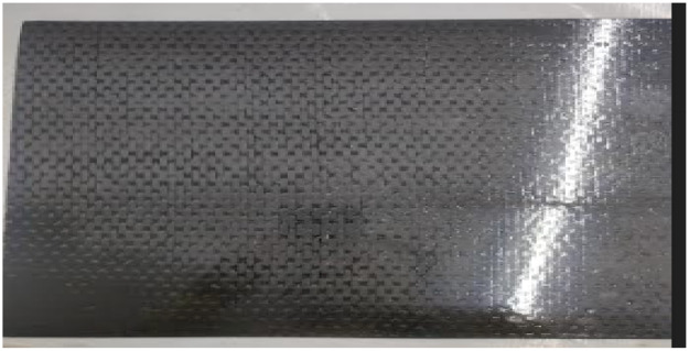
A 1.5 mm-thick carbon fibre reinforced polymers (CFRP) composite sheet was made at SP Concare Pvt. Ltd. in Sangli, Maharashtra, India, by hand-laying the material and employing epoxy resin. In order to achieve the optimal resin wetting and layer consolidation, the laminate was built using alternating layers of carbon fibre fabric. Epoxy resin was used as the matrix to construct sheets of 300 mm × 300 mm × 1.5 mm carbon-glass fibre reinforced polymer-based hybrid composites, as shown in Fig. 1.

Fig. 1.

Hybrid composites based on polymers reinforced with carbon fiber and epoxy resin.

Experiment setup

Experimentation -Laser setup and experimentation

The Trumpf TruLaser 3030 CO2 laser machine was used for trials. Various combinations of laser cutting parameters were tested, including gas pressure (2–6 bar), focal length (101.6–177.8 mm), cutting speed (100–5600 mm/min), and laser power (500–2000 W).

Parameter selection

The design factors and their corresponding levels are shown in Table 4 and are essential in figuring exactly the best settings for the laser cutting process. The quality and effectiveness of the cuts can be greatly improved by modifying important variables such gas pressure, laser power, cutting speed, and focal length. Achieving the intended outcomes in the fabrication process requires careful consideration of these factors. By maximising these variables, cutting performance is enhanced overall, accuracy is ensured, and waste material is minimised.

Table 4.

Design variables and their levels- laser cutting parameters.

Sr. No.	Symbol	Parameter	Level 1	Level 2	Level 3
1	LPW	Laser Power (W)	500	1250	2000
2	CSM	Cutting Speed (mm/min)	100	2850	5600
3	FOL	Focal Length (mm)	101.6	139.7	177.8
4	GPR	Gas pressure (bar)	2	4	6

Laser cutting procedure

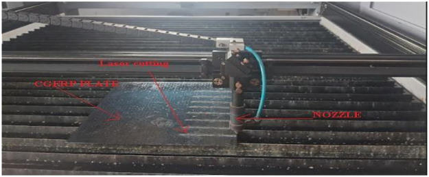
Experiments are planned once the laser cutting parameters (focal length, power, and speed) have been decided upon. The investigations aim to evaluate the cutting performance of the hybrid composite laminate and determine the optimal parameters for making precise and clean cuts. The excellent precision and control that the Trumpf TruLaser 3030 CO2 laser equipment, which is displayed in Fig. 2, The results of the experiments will provide valuable information on the characteristics of the hybrid composite material and its potential applications in many industries.

Fig. 2.

Laser setup and experimentation.

Microscope preparation

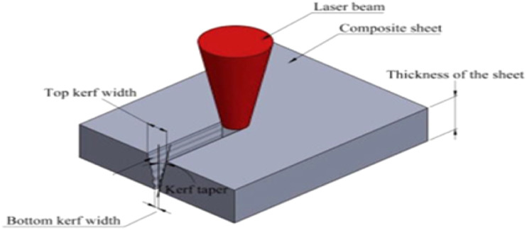
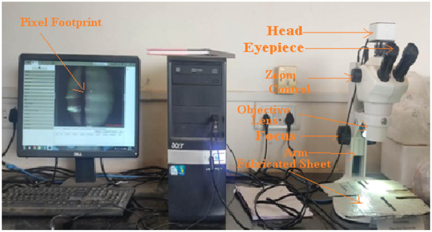
For evaluating the effectiveness of laser-cut edges, kerf quality attributes—also known as geometrical cut characteristics—is essential. Key metrics for evaluating the precision and accuracy of the cut geometry are the taper angle and kerf width (as illustrated in Fig. 3). Using a stereo zoom microscope allows for detailed visualization and measurement of kerf characteristics, providing valuable insights into the laser cutting process as shown in Fig. 4. An optical microscope is used to measure these factors in order to provide an accurate assessment. In particular, measurements are made of the following:

• •Top Kerf Width (TKW): The cutting width at the material's upper surface.
• •Bottom Kerf Width (BKFW): The breadth of the cut at the material's bottom surface is known as the bottom kerf width (BKFW).
• •Taper Angle (TPN):The angle created by the difference between the top and bottom kerf widths is known as the taper angle.

Fig. 3.

Kerf quality characteristics.

Fig. 4.

Optical microscope.

Recording and analysis

Design of Experiments (DOE)

The L27 orthogonal array facilitates a systematic approach to conducting experiments and measuring various outcomes, making it an effective tool for researching laser machining parameters. By using this array, researchers can identify significant factors affecting kerf characteristics, ultimately enhancing the precision of laser machining processes. Statistical methods such as ANOVA can be employed to analyze the data, revealing the critical influences on kerf outcomes.

Table 5 displays the outcomes of the Design of Experiments with the L27 orthogonal array. An optical microscope was used to compute BKFW, TKFW, and TPN. This experimental configuration and data analysis process enable the application of informed decisions and modifications to improve the overall efficacy and performance of the system. Several important insights that can direct future decision-making and process enhancements were found through the data analysis. It is feasible to pinpoint areas for optimization and make well-informed system modifications by applying the data acquired from the trials. All things considered, the L27 orthogonal array experiment design has yielded important insights that could improve the system's efficacy and efficiency.

Table 5.

Design of Experiments using an L27 orthogonal array with a calculation of BKFW, TKFW, and TPN using an Optical microscope.

Sr. No.	LPW (W)	CSM (mm/min)	FOL (mm)	GPR (bar)	BKFW	TKFW	TPN
1	500	100	101.6	2	0.3	0.5	2
2	500	100	139.7	4	0.35	0.55	1.5
3	500	100	177.8	6	0.4	0.6	1
4	500	2850	101.6	4	0.32	0.52	2.2
5	500	2850	139.7	6	0.37	0.57	1.8
6	500	2850	177.8	2	0.33	0.53	2.4
7	500	5600	101.6	6	0.31	0.51	2.1
8	500	5600	139.7	2	0.36	0.56	2.5
9	500	5600	177.8	4	0.38	0.58	1.9
10	1250	100	101.6	2	0.28	0.48	2.3
11	1250	100	139.7	4	0.33	0.53	2
12	1250	100	177.8	6	0.35	0.55	1.7
13	1250	2850	101.6	4	0.3	0.5	2.4
14	1250	2850	139.7	6	0.34	0.54	2.1
15	1250	2850	177.8	2	0.32	0.52	2.5
16	1250	5600	101.6	6	0.29	0.49	2.2
17	1250	5600	139.7	2	0.31	0.51	2.6
18	1250	5600	177.8	4	0.33	0.53	1.8
19	2000	100	101.6	2	0.27	0.47	2.5
20	2000	100	139.7	4	0.32	0.52	2.2
21	2000	100	177.8	6	0.34	0.54	1.9
22	2000	2850	101.6	4	0.29	0.49	2.6
23	2000	2850	139.7	6	0.33	0.53	2.3
24	2000	2850	177.8	2	0.31	0.51	2.7
25	2000	5600	101.6	6	0.28	0.5	2.8
26	2000	5600	139.7	2	0.3	0.5	2.8
27	2000	5600	177.8	4	0.32	0.52	2

The values of each design variable for maximizing the signal-to-noise ratios of BKFW, TKFW, and TPN are shown in Table 6, S/N ratio analysis for BKFW, TKFW, and TPN. These findings can help researchers adjust the system parameters to get the intended results with the least amount of unpredictability. All things considered, the thorough analysis shown in Table 5 advances knowledge of the experimental design and facilitates ongoing system performance enhancements.

Table 6.

S/N ratio analysis for BKFW, TKFW and TPN.

Sr. No	S/N ratio(BKW)	MEAN (BKFW)	S/N ratio (TKFW)	MEAN (TKFW)	S/N ratio (TPN)	MEAN (TPN)
1	10.45757	0.3	6.0206	0.5	−6.0206	2
2	9.118639	0.35	5.192746	0.55	−3.52183	1.5
3	7.9588	0.4	4.436975	0.6	0	1
4	9.897	0.32	5.679933	0.52	−6.84845	2.2
5	8.635966	0.37	4.882503	0.57	−5.10545	1.8
6	9.629721	0.33	5.514483	0.53	−7.60422	2.4
7	10.17277	0.31	5.848596	0.51	−6.44439	2.1
8	8.87395	0.36	5.036239	0.56	−7.9588	2.5
9	8.404328	0.38	4.73144	0.58	−5.57507	1.9
10	11.05684	0.28	6.375175	0.48	−7.23456	2.3
11	9.629721	0.33	5.514483	0.53	−6.0206	2
12	9.118639	0.35	5.192746	0.55	−4.60898	1.7
13	10.45757	0.3	6.0206	0.5	−7.60422	2.4
14	9.370422	0.34	5.352125	0.54	−6.44439	2.1
15	9.897	0.32	5.679933	0.52	−7.9588	2.5
16	10.75204	0.29	6.196078	0.49	−6.84845	2.2
17	10.17277	0.31	5.848596	0.51	−8.29947	2.6
18	9.629721	0.33	5.514483	0.53	−5.10545	1.8
19	11.37272	0.27	6.558043	0.47	−7.9588	2.5
20	9.897	0.32	5.679933	0.52	−6.84845	2.2
21	9.370422	0.34	5.352125	0.54	−5.57507	1.9
22	10.75204	0.29	6.196078	0.49	−8.29947	2.6
23	9.629721	0.33	5.514483	0.53	−7.23456	2.3
24	10.17277	0.31	5.848596	0.51	−8.62728	2.7
25	11.05684	0.28	6.0206	0.5	−8.94316	2.8
26	10.45757	0.3	6.0206	0.5	−8.94316	2.8
27	9.897	0.32	5.679933	0.52	−6.0206	2

Analysis of variance for S/N ratios

Analysis of variance for S/N ratios for BKFW

The variables such as LPW, CSD,FOL, and GPR significantly affect the process with p-values <0.05, suggesting strong statistical significance, according to the Analysis of Variance (ANOVA) for Signal-to-Noise (S/N) ratios for BKFW. The F-values show how important each of these elements is concerning one another, with FOL having the greatest impact and GPR, CSD, and LPW. Given the modest residual error, the majority of the data variability may be explained by the model. The overall influence of all factors and interactions is indicated by the data's total variation, which is 94.03 shown in Table 7.

Table 7.

Analysis of Variance for S/N ratios for BKFW.

Source	DF	Seq SS	Adj SS	Adj MS	F	P
LPW	2	20.99	20.99	10.4925	12.28	0.000
CSD	2	21.91	21.91	10.9556	12.82	0.000
FOL	2	1294	1294	6.4678	7.57	0.004
GPR	2	22.81	22.81	11.4044	13.34	0.000
Error	18	15.38	15.38	0.8547
Total	26	94.03

Analysis of variance for S/N ratios for TKFW

With p-values <0.05, which indicates strong statistical significance, the ANOVA Table 8 for S/N ratios for BKFW demonstrates that LPW, FOL, and GPR have a substantial impact on the process. With the highest F-values of 30.01 and 49.69, respectively, LPW and FOL are the most influential. The process is not significantly affected by CSD, as evidenced by the high p-value (0.745). The model appears to have a good representation of the data variability, based on the minimal residual error. The sum of the effects of all the components is 6.55286, which is the entire variation.

Table 8.

Analysis of Variance for S/N ratios for BKFW.

Source	DF	Seq SS	Adj SS	Adj MS	F	P
LPW	2	1.88364	1.88364	0.94182	30.01	0.000
CSD	2	0.01875	0.01875	0.00938	0.30	0.745
FOL	2	3.11871	3.11871	1.55936	49.69	0.000
GPR	2	0.96694	0.96694	0.48347	15.41	0.000
Error	18	0.56482	0.56482	0.03138
Total	26	6	6.55286

Analysis of variance for S/N ratios for TPN

Table 9 of ANOVA shows that LPW, CSD, FOL, and GPR all significantly affect the process in terms of S/N ratios for TPN. Statistical significance is indicated by P-values <0.05. The most significant variables are GPR, CSD, LPW, and FOL, based on the F-values. The relatively small inaccuracy suggests that the model might account for much of the variability in the data. The total variability is explained by the contributions of all the components and how they interact, showing the combined impact of all the components on the process.

Table 9.

Analysis of Variance for S/N ratios for TPN.

Source	DF	Seq SS	Adj SS	Adj MS	F	P
LPW	2	20.99	20.99	10.4925	12.28	0.000
CSD	2	21.91	21.91	10.9556	12.82	0.000
FOL	2	12.94	12.94	6.4678	7.57	0.004
GPR	2	22.81	22.81	11.4044	13.34	0.000
Residual Error	18	15.38	15.38	0.8547
Total	26

The quality of fit for each answer is displayed in Table 10 by the regression parameters for the constructed models. The S-value for BKFW and TPN is 0.9245, which suggests that the residuals have a moderate degree of variability. With an R2 of 83.6% for both answers, the model accounts for 83.6% of the variation in the data. The model's predictive ability is demonstrated by the adjusted R² of 76.4% for these responses, which considers the number of variables. With an R2 of 91.4% and an adjusted R2 of 87.5% for TKFW, the S-value is 0.1771, suggesting reduced residual variability and a robust fit with good predictive power.

Table 10.

Values of regression parameters for developed models.

Response	Progression Parameters
	S-value	R2 (%)	Adjusted R2(%)
BKFW	0.9245	83.6	76.4
TKFW	0.1771	91.4	87.5
TPN	0.9245	83.6	76.4

Method and validation

The validation of experimental results is a critical step in confirming the effectiveness of various machining parameters. This study employs multiple analytical methods, including Grey Relation Analysis (GRA), regression models, and Artificial Neural Networks (ANNs), to compare predicted outcomes with actual experimental results.

Grey relation analysis (GRA)

Using Grey Relational Analysis (GRA) for multi-objective optimization requires a few crucial procedures. Initially, the unprocessed data is adjusted to a similar scale, usually ranging from 0 to 1. The link between the optimal (best) and actual normalized figures is then determined using the Grey Relational Coefficient (GRC). The overall performance of each alternative is then reflected in the Grey Relational Grade (GRG), which is calculated by averaging the GRCs. The alternatives are sorted according to the GRG; greater GRG values denote superior performance. Eventually, the most GRG-valued set of parameters is chosen as the ideal set, offering a comprehensive approach to multi-objective optimization.

The formula for Grey Relational Analysis consists of multiple steps:

• Step I:

  Normalization for Every Performance Aspect:

  -Determine the maximum and minimum values for Every Column (Attribute) in the Gathered Data.

  -Use the following formula to normalize the data:

  $$p_i^{*}\left(k\right)=\frac{p_i^0\left(l\right)-min{p}_i^0\left(l\right)}{max{p}_i^0\left(l\right)-minp{f}_i^0\left(l\right)}$$

  where, $p_i^0\left(k\right)$ provides an intial sequence, $p_i^{*}\left(k\right)$ corresponds to comparability sequence, i = 1,2,3,…m (m is the total no experiment runs), $l$ =5 1,2,3,… n (n is the number of variables examined). In this study, m = 27 and n = 4 [[25], [26], [27], [28]].

• Step II:

  Determine the ideal reference sequence.

  After first step, to compute deviation sequence

  Where, $f_i^0\left(c\right)$ = reference sequence, $f_i^{*}\left(c\right)$ = comparability sequence

  $${\Delta }_{oi}c=\left|f_0^{*}\left(c\right)-f_i^{*}\left(c\right)\right|$$
• Step III:

  Calculate gray relational coefficients and grades to evaluate performance. (Finding GRC and GRG)

  It is denoted by

  $$\gamma \left[f_0^{*}\left(c\right),f_i^{*}\left(c\right)\right]=\frac{{\Delta }_{min}+\zeta .{\Delta }_{max}}{{\Delta }_{0i}\left(c\right)+\zeta .{\Delta }_{max}}$$

And 0 <$\gamma \left[x_0^{*}\left(k\right),x_i^{*}\left(k\right)\right]\le 1$

Table 11 shows the Grey Relational Rank and Grade for different sets of GPR, FOL, CSD, and LPW. The normalized values for TKFW, BKFW, and TPN are listed in each row, along with the Grey Relational Coefficients (GRC) and their respective deviation sequences. For every collection of parameters, the Grey Relational Grade (GRG) is computed and a rank is assigned based on the GRG. Better performance is indicated by higher GRG values; the combination of 2000 W LPW, 100 mm/min CSD, 101.6 mm FOL, and 2 bar GPR has the highest rank, 1.

Table 11.

Grey relational rank and grade.

LPW (W)	CSD (mm/min)	FOL (mm)	GPR (bar)	Normalized Values			Deviation Sequence			Grey Relational Coefficient			GRG	Rank
				TKFW	BKFW	TPN	TKFW	BKFW	TPN	TKFW	BKFW	TPN
500	100	101.6	2	0.77	0.77	0.44	0.23	0.23	0.56	0.7	0.7	0.5	0.63	6
500	100	139.7	4	0.38	0.38	0.72	0.62	0.62	0.28	0.4	0.4	0.6	0.46	21
500	100	177.8	6	0.00	0.00	1.00	1.00	1.00	0.00	0.3	0.3	1.0	0.53	11
500	2850	101.6	4	0.62	0.62	0.33	0.38	0.38	0.67	0.6	0.6	0.4	0.53	12
500	2850	139.7	6	0.23	0.23	0.56	0.77	0.77	0.44	0.4	0.4	0.5	0.43	25
500	2850	177.8	2	0.54	0.54	0.22	0.46	0.46	0.78	0.5	0.5	0.4	0.46	22
500	5600	101.6	6	0.69	0.69	0.39	0.31	0.31	0.61	0.6	0.6	0.5	0.56	8
500	5600	139.7	2	0.31	0.31	0.17	0.69	0.69	0.83	0.4	0.4	0.4	0.4	27
500	5600	177.8	4	0.15	0.15	0.50	0.85	0.85	0.50	0.4	0.4	0.5	0.43	26
1250	100	101.6	2	0.92	0.92	0.28	0.08	0.08	0.72	0.9	0.9	0.4	0.73	2
1250	100	139.7	4	0.54	0.54	0.44	0.46	0.46	0.56	0.5	0.5	0.5	0.5	16
1250	100	177.8	6	0.38	0.38	0.61	0.62	0.62	0.39	0.4	0.4	0.6	0.46	23
1250	2850	101.6	4	0.77	0.77	0.22	0.23	0.23	0.78	0.7	0.7	0.4	0.6	7
1250	2850	139.7	6	0.46	0.46	0.39	0.54	0.54	0.61	0.5	0.5	0.5	0.5	17
1250	2850	177.8	2	0.62	0.62	0.17	0.38	0.38	0.83	0.6	0.6	0.4	0.53	13
1250	5600	101.6	6	0.85	0.85	0.33	0.15	0.15	0.67	0.8	0.8	0.4	0.67	4
1250	5600	139.7	2	0.69	0.69	0.11	0.31	0.31	0.89	0.6	0.6	0.4	0.53	14
1250	5600	177.8	4	0.54	0.54	0.56	0.46	0.46	0.44	0.5	0.5	0.5	0.5	18
2000	100	101.6	2	1.00	1.00	0.17	0.00	0.00	0.83	1.0	1.0	0.4	0.8	1
2000	100	139.7	4	0.62	0.62	0.33	0.38	0.38	0.67	0.6	0.6	0.4	0.53	15
2000	100	177.8	6	0.46	0.46	0.50	0.54	0.54	0.50	0.5	0.5	0.5	0.5	19
2000	2850	101.6	4	0.85	0.85	0.11	0.15	0.15	0.89	0.8	0.8	0.4	0.66	5
2000	2850	139.7	6	0.54	0.54	0.28	0.46	0.46	0.72	0.5	0.5	0.4	0.46	24
2000	2850	177.8	2	0.69	0.69	0.06	0.31	0.31	0.94	0.6	0.6	0.3	0.5	20
2000	5600	101.6	6	0.92	0.77	0.00	0.08	0.23	1.00	0.9	0.7	0.3	0.7	3
2000	5600	139.6	2	0.77	0.77	0.00	0.23	0.23	1.00	0.7	.7	0.3	0.56	9
2000	5600	177.8	4	0.62	0.62	0.44	0.38	0.38	0.56	0.6	0.6	0.5	0.56	10

According to the response, Table 12 stated for the GRG, the Delta values and ranks show that FOL has the greatest impact on performance, followed by Laser Power LPW, GPR, and CSD. For each factor, the asterisks (*) indicate the ideal levels.

Table 12.

Response table for gray relational grade (GRG).

Level	LPW	CSD	FOL	GPR
1	0.4889	0.5711*	0.6411*	0.5767*
2	0.5367	0.5200	0.5089	05,378
3	0.6067*	0.5433	0.4944	0.4944
Delta	0.1178	0.0511	0.1467	0.0823
Rank	2	4	1	3

$\overline{\text{TM}}$=Total mean of the response.

The optimal ${\eta }_{opt}$ is given by

GRG ${\eta }_{opt}$ = $\overline{\text{TM}}$+[$\overline{\text{LPW}}-\overline{\text{TM}}]$ +[$\overline{\text{CSD}}-\overline{\text{TM}}]$+ [$\overline{\text{FOL}}-\overline{\text{TM}}]$+ [$\overline{\text{GPR}}-\overline{\text{TM}}]$

= 0.5481+ [0.6067–0.5481]+[0.5711–0.5481]+[0.6411–0.5481]+[0.5767–0.5481]

= 0.7510

Table 13 demonstrates that all parameters (p-values <0.05, strong statistical significance) have a significant impact on GRG, including LPW, CSD, FOL, and GPR. Combining the total mean response with the contributions of each factor at optimal values yields the ideal GRG (η_(opt)) = 0.7510 factor.

Table 13.

Analysis of variance for S/N ratios for GRG.

Source	DF	Adj.SS	Adj.MS	F-Value	P-Value
LPW	2	0.45582	0.227911	70.63	0.000
CSD	2	0.06385	0.031926	9.89	0.001
FOL	2	0.61719	0.308594	95.64	0.000
GPR	2	0.36391	0.181853	56.39	0.000
Error	18	0.05808	0.003227

As machining settings are changed from the initial to the ideal ones, Table 14's response performance data demonstrate an improvement in the GRG value from 0.78 to 0.80, validating a predicted GRG of 0.80. The GRG value has increased by 6.125% as a result.

Table 14.

Response performance results for initial and optimal settings.

	Initial Machining Parameters	Optimal Machining Parameters
		Prediction values	Experiment value
Setting Level	LPW3CSD1FOL1GPR1	LPW3CSD1FOL1GPR1	LPW3CSD2FOL1GPR2
GRG value	0.80	0.7510	0.78

Improvement of GRG = 6.125%.

Regression analysis

The regression equation is as follows.

TKFW = 0.4445 - 0.000025 LPW - 0.000001 CSD+ 0.000612 FOL + 0.00694 GPR

BKFW = 0.2449 - 0.000027 LPW - 0.000001 CSD0.000642 FOL + 0.00639 GPR

TPN= 2.704 + 0.000326 LPW + 0.000073 CSD - 0.00467 FOL - 0.1222 GPR

The association between TKFW, BKFW, and TPN with LPW, CSD, FOL, and GPR is displayed in these regression equations. The strength and direction of each variable's influence on the corresponding outcome are shown by the coefficients for each variable. We can have a better understanding of the factors impacting TKFW, BKFW, and TPN in their study by examining these equations.

ANN model

The experimental data is used to create and train an Artificial Neural Network (ANN) model. The ANN model makes predictions for various parameter combinations, which helps optimize the laser cutting procedure for improved accuracy and reduced flaws in CGFRP composites. Improved cutting efficiency and quality in CGFRP composite materials are the result of a thorough optimization method made possible by the integration of Taguchi analysis and ANN forecasts

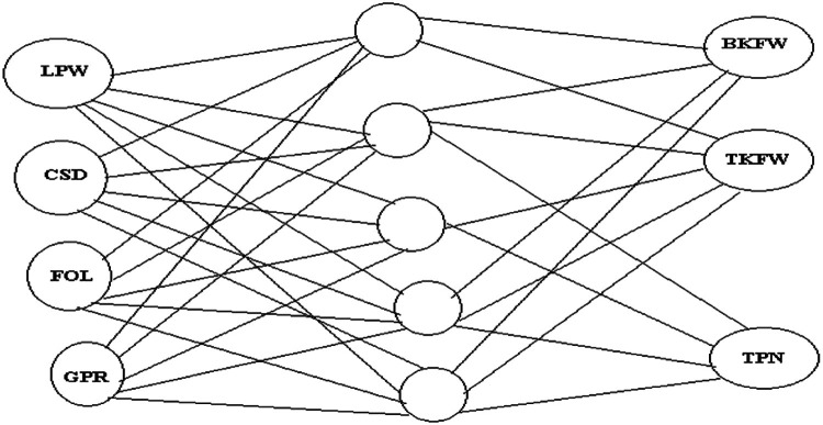
Fig. 5 shows an Artificial Neural Network (ANN) model with three output responses (BKFW, TKFW, TPN) and four input parameters (LPW, CSD, FOL, and GPR). The intricate relationships and interactions between the machining settings and the final performance measures are illustrated by the hidden layer, which links the inputs and outputs.

• •Setting up the data set: Determining certain input features and output targets is the initial stage in creating an Artificial Neural Network (ANN) model. Gas Pressure (GPR) in bar, Focal Length (FOL) in mm, Cutting Speed (CSD) in mm/min, and Laser Power (LPW) in watts are important input characteristics. Three output targets are intended to be predicted by the model: Taper (TPN), Top Kerf Width (TKFW), and Bottom Kerf Width (BKFW). An input layer with four neurones (one for each input feature), one or two hidden layers with ten to twenty neurones each (the ideal number was established through testing), and an output layer with three neurones for the output variables constitute the ANN structure.
• •Data Set Division: In order to facilitate efficient training and assessment, the data set should next be split up into discrete subsets. About 10–15% (or about 4 points) of the data are usually set aside as the validation set for hyper parameter adjustment, and the remaining 70–80% of the data (or about 19 points) serve as the training set. The testing set for the final evaluation consists of the remaining 10–15% (about 4 points). Using k-fold cross-validation can improve the generalization of the model even more.
• •Hyperparameter tuning: This is an additional important factor that includes modifying the network width, depth, and learning rate. Batch sizes are usually set to 16 or 32, and initial learning rates are set at small values (0.001 or 0.01). Six epochs of training are typically required, and early termination techniques are used to avoid overfitting.
• •Architecture of the model: In terms of the ANN's performance, it is essential. Four neurons make up the input layer, one for each of the recognized input characteristics. The ideal configuration of the model, which usually consists of 1–2 hidden layers with 10–20 neurons each, is worked out through testing. Three neurons make up the output layer, one for each of the output targets.

Fig. 5.

ANN model.

Furthermore, measurements for performance evaluation that help determine the accuracy of the model include Mean Absolute Error (MAE) and Root Mean Squared Error (RMSE). An accurate indicator of the model's predictive reliability can be obtained by contrasting ANN forecasts for BKFW, TKFW, and TPN with experimental findings as shown in Table 15.

Table 15.

ANN model results summary.

Set	Observations	MSE	RMSE	R-squared (R)
Training Set	21	0.00002492	0.004992	0.9855
Validation Set	2	0.0018	0.042426	1
Test Set	2	0.00009059	0.009518	1
Additional Test Set	2	0.00038148	0.019532	0.8525

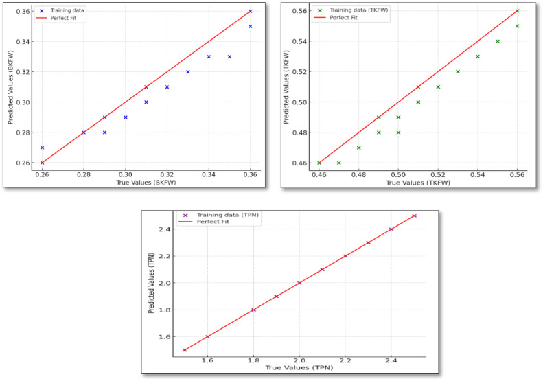
Each plot of Fig. 6 illustrates the relationship between the actual and predicted values for BFKW,TFKW and TPN, with the red line indicating the fitted regression line and the blue dashed line representing the ideal case where predicted values perfectly match the actual values.

Fig. 6.

Trained model's regression plots for a) BKFW, b) TKFW, and c) TPN.

The Levenberg-Marquardt Algorithm (LMA) is an effective optimization technique for training feed forward neural networks. To determine optimal epoch values, you can analyze the training log, which records performance metrics like MSE and RMSE for each epoch. Implementing early stopping criteria can also help identify when training should cease, providing a clear optimal epoch value. Additionally, performance plots can visually reveal the epoch with minimal validation error before over fitting occurs, the best validation performance of MSE 0.0018338 was achieved at epoch 3.

Table 16 displays the design of the experiments using an L27 orthogonal array to obtain values from the ANN model using BKFW, TPN, and TKFW. The results demonstrate how well Artificial Neural Network (ANN) models function to forecast and optimize laser machining parameters for hybrid composites, with a particular emphasis on reducing TPN, TKFW, and BKFW. Its dependability emphasizes how useful it is for directing laser-cutting process improvement tactics.

Table 16.

Design of experiments with utilizing with BKFW,TPN and TKFW an L27 orthogonal array obtain the values from ANN model.

Sr. No.	LPW (W)	CSD (mm/min)	FOL (mm)	GPR (bar)	BKFW	TKFW	(TPN)
1	500	100	101.6	2	0.29	0.49	1.9
2	500	100	139.7	4	0.33	0.53	1.6
3	500	100	177.8	6	0.36	0.56	1.5
4	500	2850	101.6	4	0.31	0.51	2.0
5	500	2850	139.7	6	0.35	0.55	1.8
6	500	2850	177.8	2	0.32	0.52	2.1
7	500	5600	101.6	6	0.30	0.50	2.2
8	500	5600	139.7	2	0.34	0.54	2.3
9	500	5600	177.8	4	0.36	0.56	1.9
10	1250	100	101.6	2	0.26	0.47	2
11	1250	100	139.7	4	0.30	0.50	1.8
12	1250	100	177.8	6	0.33	0.53	1.5
13	1250	2850	101.6	4	0.29	0.49	2.1
14	1250	2850	139.7	6	0.32	0.52	1.9
15	1250	2850	177.8	2	0.30	0.50	2.2
O0-	1250	5600	101.6	6	0.28	0.48	2.3
17	1250	5600	139.7	2	0.31	0.51	2.4
18	1250	5600	177.8	4	0.33	0.53	1.8
19	2000	100	101.6	2	0.26	0.46	2.5
20	2000	100	139.7	4	0.29	0.49	2.1
21	2000	100	177.8	6	0.31	0.51	1.9
22	2000	2850	101.6	4	0.27	0.47	2.2
23	2000	2850	139.7	6	0.30	0.50	2.0
24	2000	2850	177.8	2	0.28	0.48	2.4
25	2000	5600	101.6	6	0.26	0.46	2.5
26	2000	5600	139.7	2	0.28	0.48	2.6
27	2000	5600	177.8	4	0.30	0.50	1.9

Comparison of experimentation and ANN method

CSD and lower LPW are identified in the study as critical variables for lowering BKW and TKW while preserving material integrity. As an example, installations with 500 W of LPW and 2850 mm/min of CSD show consistently lower BKW and TKW when compared to higher LPW settings. This association highlights how crucial it is to optimize these factors to have accurate cuts with small kerf widths. Lower values of TPN, which represents the degree of tapering in cuts, correspond to more accurate cutting. Based on experimental data, TPN can be greatly influenced by combinations of LPW, CSD, FOL, and GPR). A TPN value of 1.5, for instance, can be attained with particular parameters like LPW of 500 W, CSD of 100 mm/min, FOL of 177.8 mm, and GPR of 6 bar, demonstrating the intricate interaction of variables in obtaining the best possible cutting quality. GPR has a significant effect on the results of machining; higher pressures are often associated with lower BKW and TKW as a result of better thermal management and material evacuation. To avoid potential surface damage or excessive material loss, it is essential to use caution when balancing GPR with other parameters. This emphasizes the need for a thorough approach to parameter selection.

Comparison between experimental –BFKW and ANN model –BFKW

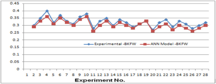
The experimental findings for BFKW and the ANN model predictions, as illustrated in Fig. 7, exhibit a significant trend resemblance. This suggests that the ANN model is quite good at properly predicting the results of the experiments. The alignment between the two lines further validates the ANN model's reliability and precision in this setting.

Fig. 7.

Comparison between experimental –BFKW and ANN Model –BFKW.

Comparison between experimental –TKFW and ANN model -TKFW

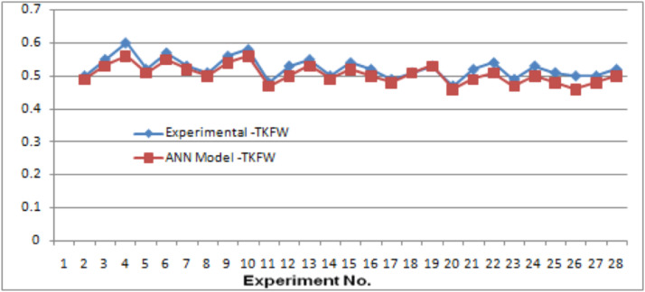
Fig. 8 depicts a comparison of experimental results and ANN model predictions for TKFW. The model predictions closely match the experimental data, proving the model's reliability in this context as well.

Fig. 8.

Comparison between experimental –TKFW and ANN Model -TKFW.

Comparison between experimental –TPN and ANN model -TPN

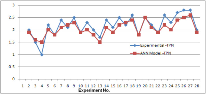
Fig. 9 between the two data sets, with just small differences detected. This indicates that the ANN model can accurately predict TPN values based on experimental data.

Fig. 9.

Comparison between experimental –TPN and ANN Model -TPN.

Result and discussion

To validate the results, the experimental data were compared to the predictions made using regression models, artificial neural networks (ANNs), and grey relation analysis (GRA).

• •
  Grey relation analysis (GRA)

  • ○
    Compare the GRG values from the initial setup and the optimized setup to check for improvement.
  • ○
    The initial GRG value was 0.78, while the predicted optimal GRG was 0.7510.
  • ○
    After running the experiment with the optimized parameters, the final GRG was found to be 0.80, showing an improvement over both the initial and predicted values.
  • ○
    By demonstrating a 0.23% improvement in GRG and validating its significance through statistical analysis, it enhances the validity and applicability of their finding
• •Regression analysis models
• •It is essential for investigating the relationships between various machining elements (such LPW, CSD, FOL, and GPR) and results.
• •Through this analysis confirmed the validity of the results of the investigation and provides opportunities for more research and experimentation in the field of machining.
• •Artificial Neural Network (ANN)
• •The performance of the model is checked through metrics such as the R-value and Mean Squared Error (MSE) to ensure accurate predictions and reliable optimization.
• •The ANN model predicts BKFW, TKFW, and TPN values with a high degree of accuracy. Thus, the ANN model's overall accuracy is roughly 93.48%.For optimization purposes, the model is deemed credible as the projected values exhibit a high degree of agreement with the observed values.

Conclusions

Several significant issues are usually included at the end of the investigation on utilizing Taguchi optimization and ANN-based optimization to improve laser cutting precision for CGFRP composites.

• •Through the design of trials that assess the relationships between input parameters (like CSD, LPW, FOL, and GPR) and output parameters (like TKWF, BKWF, and TPN), Taguchi Optimization effectively identifies the optimal laser cutting settings.
• •Using Grey Reduction Analysis (GRA) makes it easier to determine the ideal machining parameters that strike a compromise between competing goals, like improving material integrity and surface quality and minimizing kerf width (BKW, TKW), taper angle (TPN), and other factors.
• •The experimentation shows that higher CSD (mm/min) and lower LPW (W) tend to minimize BKW and TKFW, indicating that the model can assist in determining the best parameters for decreasing TPN.
• •A combination of lower LPW (e.g., 500 W), greater CSD (e.g., 2850 mm/min), and higher GPR (e.g., 6 bar) should be taken into consideration in order to achieve minimal BKFW, TKFW, and TPN.
• •The development of an Artificial Neural Network (ANN) effectively captures the complex relationships between machining settings and performance outcomes.

Limitations

• •On carbon-glass hybrid composites, changing LPW and CSD too much might result in flaws including burn markings, ragged edges, and thermal damage.
• •The complex interactions between the resin and the diverse properties of carbon and glass fibers can impact surface integrity and cutting efficiency.
• •Getting consistent surface quality across different composite types and thicknesses can be challenging, leading to precise control and optimization of laser parameters.

Ethics statements

Not applicable.

Supplementary material and/or additional information [OPTIONAL]

NA.

CRediT authorship contribution statement

Ashish A Desai: Conceptualization, Methodology, Software, Writing – original draft. S.N. Khan: Supervision. Pooja Bagane: Visualization, Investigation. Sagar Dnyandev Patil: Writing – review & editing.

Declaration of competing interest

The authors declare that they have no known competing financial interests or personal relationships that could have appeared to influence the work reported in this paper.

Data availability

Data will be made available on request.

References

- 1.Hiwale S., Rajiv B. Experimental investigations of laser machining process parameters using response surface methodology. Mater. Today Proc. 2021;44(6):3939–3945. doi: 10.1016/j.matpr.2020.09.295. PartISSN 2214-7853. [DOI] [Google Scholar]
- 2.Patil S.D. Multi-objective optimization of carbon/glass hybrid composites with newly developed resin (NDR) using gray relational analysis. Multidiscip. Model. Mater. Struct. 2020;16(6):1709–1729. doi: 10.1108/MMMS-08-2019-0141. ISSN 1573-6105. [DOI] [Google Scholar]
- 3.Tabar M.Y., Hashemzadeh M., Rejani A.R. CO2 laser cutting of reinforced polyester (CGFRP and GFRP) sheets: an experimental investigation into specific point energy, cutting volume efficiency and material removal rate (MRR) J. Manuf. Process. 2023;97:137–147. doi: 10.1016/j.jmapro.2023.04.059. ISSN 1526-612. [DOI] [Google Scholar]
- 4.Li M., Chen L., Yang X. A feasibility study on high-power fiber laser cutting of thick CFRP laminates using single-pass strategy. Opt. Laser Technol. 2021;138 doi: 10.1016/j.optlastec.2020.106889. 106889,ISSN 0030-3992. [DOI] [Google Scholar]
- 5.Chen M., Guo B., Jiang L., Liu Z., Qian Q. Analysis and optimization of the heat affected zone of CFRP by femtosecond laser processing. Opt. Laser Technol. 2023;167 doi: 10.1016/j.optlastec.2023.109756. 109756,ISSN 0030-3992. [DOI] [Google Scholar]
- 6.Huang S., Fu Z., Liu C., Li J. Multi-objective optimization of fiber laser cutting quality characteristics of glass fiber reinforced plastic (GFRP) materials. Opt. Laser Technol. 2023;167 doi: 10.1016/j.optlastec.2023.109720. 109720,ISSN 0030-3992. [DOI] [Google Scholar]
- 7.Huang S., Fu Z., Liu C., Wang C. Interactional relations between ablation and heat affected zone (HAZ) in laser cutting of glass fiber reinforced polymer (GFRP) composite by fiber laser. Opt. Laser Technol. 2023;158 doi: 10.1016/j.optlastec.2022.108796. Part A108796,ISSN 0030-3992. (2023) [DOI] [Google Scholar]
- 8.Solati A., Hamedi M., Safarabadi M. Combined GA-ANN approach for prediction of HAZ and bearing strength in laser drilling of GFRP composite. Opt. Laser Technol. 2019;113:104–115. doi: 10.1016/j.optlastec.2018.12.016. ISSN 0030-3992. [DOI] [Google Scholar]
- 9.Nagesh S., Narasimha Murthy H.N., Pal R., Krishna M., Satyanarayana B.S. Influence of nanofillers on the quality of CO2 laser drilling in vinylester/glass using Orthogonal Array Experiments and Grey Relational Analysis. Opt. Laser Technol. 2015;69:23–33. doi: 10.1016/j.optlastec.2014.12.002. ISSN 0030-3992. [DOI] [Google Scholar]
- 10.Nagesh S., Narasimha Murthy H.N., Krishna M., Basavaraj H. Parametric study of CO2 laser drilling of carbon nanopowder/vinylester/glass nanocomposites using design of experiments and grey relational analysis. Opt. Laser Technol. 2013;48:480–488. doi: 10.1016/j.optlastec.2012.11.013. ISSN 0030-3992. [DOI] [Google Scholar]
- 11.Mishra L., Mishra D., Ranjan Mahapatra T. Optimization of process parameters in Nd:YAG laser micro-drilling of graphite/epoxy based polymer matrix composite using Taguchi based Grey relational analysis. Mater. Today Proc. 2022;62:7467–7472. doi: 10.1016/j.matpr.2022.03.501. Part 14ISSN 2214-7853. [DOI] [Google Scholar]
- 12.Rejani A.R., Hashemzadeh M. CO2 laser-air cutting of glass-fibre-reinforced unsaturated polyester (GFRUP): an experimental investigation. Int. J. Adv. Manuf. Technol. 2022;117 doi: 10.1007/s00170-021-07180-6. 2627–2638,(2022) [DOI] [Google Scholar]
- 13.Alhawsawi AM., Moustafa EB., Fujii M., Banoqitah E.M., Elsheikh A. Kerf characteristics during CO2 laser cutting of polymeric materials: experimental investigation and machine learning-based prediction. Eng. Sci. Technol. Int. J. 2022;46 doi: 10.1016/j.jestch.2023.101519. 101519,ISSN 2215-0986. [DOI] [Google Scholar]
- 14.Tabar M.Y., et al. CO2 laser cutting of reinforced polyester (CGFRP and GFRP) sheets: an experimental investigation into specific point energy, cutting volume efficiency and material removal rate (MRR) J. Manuf. Process. 2023;97:137–147. doi: 10.1016/j.jmapro.2023.04.059. [DOI] [Google Scholar]
- 15.Dutt Gautam G., Pandey A.K. Teaching learning algorithm based optimization of kerf deviations in pulsed Nd:YAG laser cutting of Kevlar-29 composite laminates. Infrared Phys. Technol. 2020;89:203–217. doi: 10.1016/j.infrared.2017.12.017. ISSN 1350-4495. [DOI] [Google Scholar]
- 16.Vishnu Vardhan T., Mahender T. Optimization of laser beam cutting machining parameters using ANOVA and regression models. Electrochem. Soc. 2022;107(1):14975. doi: 10.1016/j.matpr.2023.02.189. Inc. [DOI] [Google Scholar]
- 17.Gautam G.D., Mishra D.R. Dimensional accuracy improvement by parametric optimization in pulsed Nd:YAG laser cutting of Kevlar-29/basalt fiber-reinforced hybrid composites. J. Braz. Soc. Mech. Sci. Eng. 2019;41:1–22. doi: 10.1007/s40430-019-1783-y. [DOI] [Google Scholar]
- 18.Raza M.S., Datta S. Parametric study of laser cutting of carbon fibre reinforced polymer (CFRP) and the effect of fibre orientation on cutting quality. Adv. Mater. Process. Technol. 2019;5(2):202–212. doi: 10.1080/2374068X.2018.1564865. [DOI] [Google Scholar]
- 19.Patil S.D., Hatte P., Khan S.N., Desai A.A., Yadav P.H. Analyzing the design parameters and their influence on the tensile strength of composite layers using Taguchi technique. Mater. Today Proc. 2022;77:640–646. doi: 10.1016/j.matpr.2022.11.276(2022). Part 32023ISSN 2214-7853. [DOI] [Google Scholar]
- 20.Antonio R., Félix Q., Fernando L., Rafael C., Mohamed B., Juan P. Experimental study on the CO2 laser cutting of carbon fiber reinforced plastic composite. Compos. Part A Appl. Sci. Manuf. 2012;43(8):1400–1409. doi: 10.1016/j.compositesa.2012.02.012. [DOI] [Google Scholar]
- 21.Patil S.D., Chavan D.S., Kavade M.V. Investigation of composite torsion shaft for torsional buckling analysis using finite element analysis. IOSR J. Mech. Civ. Eng. 2012;4(3):26–31. doi: 10.9790/1684-0432631. [DOI] [Google Scholar]
- 22.Mathew J., Goswami G.L., Ramakrishnan N., Naik N.K. Parametric studies on pulsed Nd:YAG laser cutting of carbon fibre reinforced plastic composites. J. Mater. Process. Technol. 1999;89–90:198–203. doi: 10.1016/S0924-0136(99)00011-4. VolumesISSN 0924-0136. [DOI] [Google Scholar]
- 23.Patil S.D., Bhalerao Y.J. Optimization of dynamic properties of hybrid composite shaft with newly developed resin (NDR) using grey relational analysis. Int. J. Struct. Integr. 2020;11(2):248–263. doi: 10.1108/IJSI-07-2019-0073. [DOI] [Google Scholar]
- 24.Patil SD., Chavan D.S., Kavade M.V. Investigation of composite torsion shaft for static structural analysis using finite element analysis. Int. J. Eng. Res. Technol. 2012;1(7):1–5. doi: 10.17577/IJERTV1IS7186. [DOI] [Google Scholar]
- 25.Patil S.D., Bhalerao Y. Optimization of design variables for carbon/glass hybrid composites laminates using Taguchi Technique. World J. Eng. 2020;17:309–323. doi: 10.1108/WJE-10-2019-0290. [DOI] [Google Scholar]
- 26.Khot A.B., Patil S.D., Patil V.S. Analyzing the effect of process parameters on amaranth popping and puffing in the Lahi machine using the Taguchi method. J. Phys. Conf. Ser. 2023;2601 doi: 10.1088/1742-6596/2601/1/012013. - [DOI] [Google Scholar]
- 27.Patil S.D., Khot A.B., Hatte P.R. Multi-objective optimization and development of mathematical model for process parameters of AmaranthGrains using regression analysis. Res. Sq. 2024 doi: 10.21203/rs.3.rs-3852631/v1. [DOI] [Google Scholar]
- 28.Badie M.A., Mahdi E., Hamouda A.M.S. An investigation into hybrid carbon/glass fiber reinforced epoxy composite automotive drive shaft. Mater. Des. 2011;32(3):1485–1500. doi: 10.1016/j.matdes.2010.08.042. [DOI] [Google Scholar]
Associated Data
This section collects any data citations, data availability statements, or supplementary materials included in this article.
Data Availability Statement