Learning structural heterogeneity from cryo-electron sub-tomograms with tomoDRGN

Abstract

Cryo-electron tomography (cryo-ET) enables observation of macromolecular complexes in their native, spatially contextualized cellular environment. Cryo-ET processing software to visualize such complexes at nanometer resolution via iterative alignment and averaging are well-developed but rely upon assumptions of structural homogeneity among the complexes of interest. Recently developed tools allow for some assessment of structural diversity but have limited capacity to represent highly heterogeneous structures, including those undergoing continuous conformational changes. Here we extend the highly expressive cryoDRGN deep learning architecture, originally created for single particle cryo-electron microscopy analysis, to cryo-ET. Our new tool, tomoDRGN, learns a continuous low-dimensional representation of structural heterogeneity in cryo-ET datasets while also learning to reconstruct heterogeneous structural ensembles supported by the underlying data. Using simulated and experimental data, we describe and benchmark architectural choices within tomoDRGN that are uniquely necessitated and enabled by cryo-ET. We additionally illustrate tomoDRGN’s efficacy in analyzing diverse datasets, using it to reveal high-level organization of HIV capsid complexes assembled in virus-like particles and to resolve extensive structural heterogeneity among ribosomes imaged in situ.

INTRODUCTION

An array of large, dynamic macromolecular complexes carry out essential cellular functions. The conformational flexibility and compositional variability in these complexes allow cells to mount targeted molecular responses to various stresses and stimuli. Structural biology has long aimed to visualize these diverse structures with the goals of gaining mechanistic insights into these responses and testing hypotheses related to macromolecular structure-function relationships. In pursuit of this goal, cryo-electron microscopy (cryo-EM) has proven to be a powerful tool for visualizing purified complexes with high resolution^1,2. In cryo-EM, ~10⁴ - 10⁷ individual particles are imaged, each from a single unknown projection angle. Single particle analysis (SPA) is then used to simultaneously estimate the most likely projection angle for each particle image and the k ≥1 distinct 3-D volumes of the target complex, which, when projected to 2-D, are most likely to have produced the source dataset³. More recently, a number of tools have leveraged SPA datasets to deeply explore structural heterogeneity within these complexes^4–8, dramatically expanding the range of insights and testable biological hypotheses that can be derived from cryo-EM⁹.

Cryo-electron tomography (cryo-ET) is a related imaging modality wherein a sample is repeatedly imaged from several known projection angles, enabling the reconstruction of a 3-D tomogram¹⁰. As such, cryo-ET disentangles particles that overlap along a projection axis and enables the nanometer-scale 3-D visualization of highly complex samples, including subcellular volumes. Thus, cryo-ET affords the opportunity to inspect macromolecular structures in their native cellular context^11–14, in contrast with cryo-EM’s typical requirement that particles be isolated from cells and purified.

Sub-tomogram averaging (STA), a particle averaging approach analogous to SPA, is often employed in cryo-ET data processing. In STA, individual 3-D volumes, each a sub-tomogram corresponding to a unique particle, are extracted from the back-projected tilt series and are iteratively aligned to produce an average particle volume with increased signal-to-noise ratio (SNR) and resolution^15–25. Recent developments in STA processing have dramatically improved the attainable resolution through more detailed and robust modeling of physical and optical parameters even for samples in situ^26–29. Critically, STA can therefore offer insights into native protein complexes, and generate new hypotheses for molecular mechanisms by identifying unknown associated factors or novel complex ultrastructure. For example, STA has very recently been employed to extensively characterize numerous structural states of the ribosome life cycle in situ^{12–14,30–32}.

Similar to SPA, several tools have been developed to characterize heterogeneity among individual particles relative to the global average, either during or after STA^{19,29,33–35}. Although these approaches have proven fruitful in answering specific biological questions such as nucleosome flexibility^33,34, and ribosome heterogeneity^12,29, each approach has specific constraints that limit their generality. For example, sub-tomogram principal component analysis (PCA)²⁹ assumes heterogeneity can be modeled as a linear combination of voxel intensity; normal mode analysis³⁴ requires a priori knowledge of an atomic model or density map to compute normal modes; and optical flow³³ is inherently limited to conformational changes of the target particle in which the total voxel intensity across each sub-tomogram remains approximately constant. An unbiased and expressive tool to analyze heterogeneity is therefore highly desirable, particularly for in situ discovery of unexpected cofactors whose identity, binding site, and occupancy may be unknown.

Here, we introduce tomoDRGN (Deep Reconstructing Generative Networks), a deep learning framework designed to learn a continuously generative model of per-particle conformational and compositional heterogeneity from cryo-ET datasets. TomoDRGN is related to our well-characterized cryoDRGN software^4,8, and therefore shares many overall design, processing, and analysis philosophies. As input, tomoDRGN uses 2-D particle projection images and corresponding metadata from upstream STA tools (Fig. 1a), a data type used in a number of recently developed approaches^{12,27–29,36,37}. It then learns to simultaneously embed each particle within a continuous low dimensional latent space and to reconstruct the corresponding unique 3-D volume (Fig. 1b). We have additionally developed and integrated software tools to visualize and interpret these outputs, and to prepare tomoDRGN outputs for subsequent analyses with external processing software, including contextualizing the tomoDRGN generated volumes within the in situ cellular tomography data.

Figure 1: A neural network architecture to analyze structurally heterogeneous particles imaged by cryo-ET.

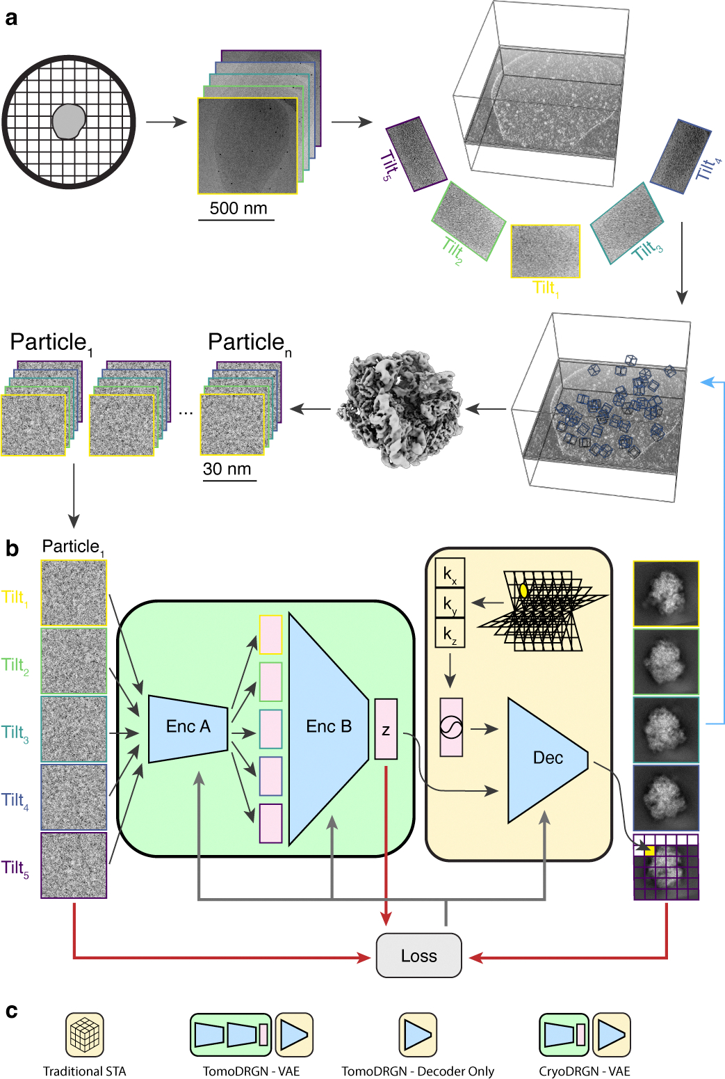
(a) A typical sample and data processing workflow to produce tomoDRGN inputs. The sample (e.g., a bacterial cell) is applied to a grid, plunge frozen, and optionally thinned. A series of TEM images of a target region are collected at different stage tilts. A tomographic volume is reconstructed using weighted back-projection of all tilt images. Instances of the target particle are identified (blue boxes) and extracted as 3-D voxel arrays. Iterative sub-tomogram averaging (STA) is used to reconstruct a consensus density map. Per-particle 2-D tilt images are then re-extracted from the source tilt series images and parameters (e.g. pose, defocus, etc.) estimated from STA are associated with the images.

(b) The tomoDRGN network architecture and training design. Each particle’s set of tilt images are independently passed through Encoder A, then jointly passed through Encoder B, thereby mapping all tilt images of a particle to one embedding (z) in a low dimensionality latent space. The decoder network (Dec) uses the latent embedding and a featurized voxel coordinate to decode a corresponding set of images pixel-by-pixel. Note that the decoder can learn a homogeneous structure by excluding the encoder module (green). The network is trained using a loss function (grey arrows) that depends on the input images, reconstructed images, and z (red arrows).

(c) Graphical signposts for volumes generated or analyzed by different reconstruction tools. These signposts are used throughout this manuscript when volumes are displayed to clarify how they were generated.

RESULTS

Network design for heterogeneous cryo-ET reconstructions

TomoDRGN was designed to efficiently train a neural network capable of: 1) embedding a collection of particles, which are each represented by multiple images collected at different stage tilt angles, to a learned, continuous, low-dimensional latent space informed by structural heterogeneity; and 2) generating a 3-D volume for each particle using these embeddings. By design, cryoDRGN is unsuited for this task as it maps individual images to unique latent embeddings, which is expected for cryo-EM single particle datasets. Thus, cryoDRGN is not constrained to map differentially tilted images of the same particle to consistent regions of latent space, leading to uninterpretable learned latent spaces and generated volumes (see Discussion).

To handle tilt-series data, we employed a variational autoencoder (VAE) framework³⁸, and constructed a purpose-built two-part encoder network feeding into a coordinate-based decoder network^39,40 (Fig. 1b). For each particle, the encoder network first uses encoder A (per tilt image) as a “feature extractor” to generate a unique intermediate embedding for each tilt image in a manner directly analogous to cryoDRGN’s encoder network. Encoder B then integrates these intermediate embeddings into a single latent embedding for the particle. The decoder network is supplied with this integrated latent embedding and a featurized voxel coordinate to reconstruct the signal at that coordinate. As in cryoDRGN, these operations are performed in reciprocal space. With this design, we expected that repeatedly evaluating the decoder network at multiple coordinates would allow for a rasterized reconstruction of the set of tilt images originally supplied to the encoder. Following a standard VAE³⁸, we designed the network to be trained by minimizing a reconstruction loss between input and reconstructed images, and a latent loss quantified by the KL-divergence of the latent embedding from a standard normal distribution, with a hyperparameter β controlling the relative contributions of these two loss terms⁴¹.

Once trained, we expected a tomoDRGN network to enable detailed and systematic interrogation of structural heterogeneity within the input dataset. For example, similar to cryoDRGN, we expected that tomoDRGN’s learned latent space could be visualized either directly along any sets of latent dimensions or using a dimensionality reduction technique such as UMAP⁴², where we have empirically found that distinct clusters often correspond to compositionally heterogeneous states, and diffuse, unfeatured distributions correspond to continuous structural variation⁸. Latent embeddings, sampled individually or following a well-populated path in latent space, could then be passed to the decoder to generate corresponding 3-D volumes for direct visualization. We predicted additional analysis could then be performed in 3-D voxel space using standard cryoDRGN tools⁹. We also constructed interactive tools to visualize and analyze heterogeneity in the spatial context of the original tomograms. Finally, we further developed methods to isolate particle subsets of interest for subsequent refinement with traditional STA software (Fig. 1c) as an iterative approach to maximize the value of a tomographic dataset.

Sub-tomogram-specific image processing approaches

Having conceived the general tomoDRGN framework, we next considered additional image processing procedures that we hypothesized might improve model quality and computational performance. First, we noted that STA software tools commonly implement weighting schemes to model the signal-to-noise (SNR) of each image as a function of the image tilt angle, which impacts the electron pathlength through the sample and cumulative electron dose, which causes accumulated radiation damage^27,43,44. Thus, we followed standard formulations for tilt weighting as the cosine of the stage tilt and dose weighting using fixed exposure curves, and we incorporated such weights into the reconstruction error calculated in tomoDRGN’s decoder network (Extended Data Fig. 1a,b). We expected such an approach would effectively downweigh the reconstruction loss of highly tilted and radiation damaged images, particularly at high frequencies.

Second, tomoDRGN’s coordinate-based decoder is trained by evaluating a set of spatial frequencies per tilt image that, by default, is identical for all tilt images and thus independent of cumulative dose imparted at each tilt. However, prior work has shown that the SNR at a given spatial frequency can be maximized at an optimal electron dose⁴⁵ and that during cryo-EM movie alignment, filtering spatial frequencies in each frame by their optimal dose can improve the aligned micrograph quality^43,46. We therefore implemented a scheme applying optimal dose filtering to Fourier coordinates evaluated by the decoder during model training (Extended Data Fig. 1a,b). We expected that such filtering would restrict the set of spatial frequencies evaluated during decoder training without sacrificing 3-D reconstruction accuracy, thereby decreasing the computational burden of model training, particularly for high resolution datasets at large box sizes.

Finally, real-world datasets frequently contain particles missing some tilt images, often due to upstream micrograph filtering (Extended Data Fig. 2a). To flexibly handle such nonuniform input data, we implemented an approach that surveys the dataset for the fewest tilt images associated with a single particle (n), then randomly samples n tilt images from each particle during model training and evaluation (Extended Data Fig. 2b, see Methods). Because this approach subsets and permutes tilt images at random, encoder B must learn a permutation-invariant function mapping from encoder A’s output (per tilt image) to the final latent space (per particle), and we hypothesized that this permutation-invariant learning goal might provide added regularization that could decrease overfitting by our model.

TomoDRGN recovers simulated structural heterogeneity

To judge the efficacy of these architectural choices, we simulated⁴⁷ cryo-ET particle stacks corresponding to four assembly states (B-E) of the bacterial ribosome large subunit (LSU)^48,49 (Fig. 2a). We initially tested the ability of the isolated decoder network to perform a homogeneous reconstruction of the class E particles wherein no encoder was trained, and no latent space was learned. We observed rapid convergence of the decoder network, with it reproducing the ground-truth density maps within 10 epochs of training (Fig. 2b).

Figure 2: TomoDRGN recovers compositional and conformational heterogeneity in simulated datasets.

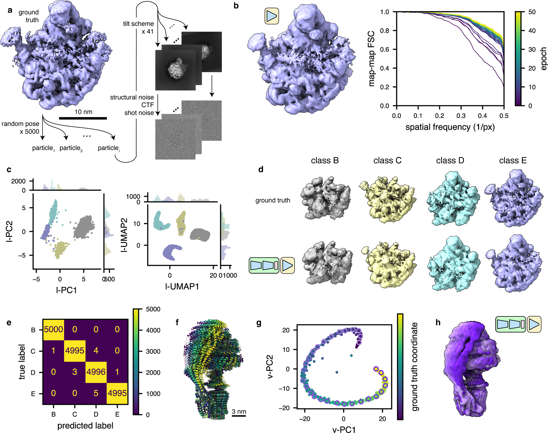
(a) Illustration of the method used to simulate tilt series particle stacks corresponding to four assembly states (B-E) of the bacterial large ribosomal subunit⁴⁸.

(b) Left, a tomoDRGN homogeneous network reconstruction of the simulated class E dataset after 50 epochs of training using simulated images with a Nyquist resolution limit of 7.1 Å. Right, Fourier Shell Correlation between the tomoDRGN reconstruction and the ground truth volume at each of 50 epochs of training (purple to yellow).

(c) First two principal components (left) and UMAP embeddings (right) of tomoDRGN latent space when trained on the simulated four class dataset, colored by k=4 k-means classification of latent space.

(d) Ground truth ribosomal volumes (top) and corresponding tomoDRGN-reconstructed volumes (bottom) sampled from the median latent encoding of each of the k=4 k-means classes in (c).

(e) Confusion matrix of k-means clustering class labels from (c) against ground truth class labels.

(f) Superposition of yeast mitochondrial ATP synthase structures undergoing conformational changes during ATP hydrolysis⁵⁰. Maps are colored purple to yellow along the simulated reaction coordinate.

(g) Voxel-based principal component analysis (vPCA)⁹ of 500 tomoDRGN-generated volumes sampled from a tomoDRGN model trained on the simulated ATP synthase dataset from panel (f). Points corresponding to each of the 500 tomoDRGN-generated volumes are colored according to their position along the simulated ground-truth reaction coordinate (see color scale). A subset of 30 such maps are sampled along the trajectory and outlined with a pink-to-purple color gradient, and these maps are presented in Supplementary Movie 1.

(h) Superposition of 6 tomoDRGN-generated volumes sampled down the continuous coordinate visualized in panel (g) and colored accordingly.

To assess tomoDRGN’s ability to faithfully embed and reconstruct structurally heterogeneous 3D volumes, we next trained the full VAE network using particle stacks containing a mixture of all four LSU structural classes. After training for 24 epochs, we observed four distinct clusters of latent embeddings by PCA and UMAP (Fig. 2c). Furthermore, the decoder network generated volumes from the center of each latent cluster that were consistent with the ground truth volumes (Fig. 2d). Finally, we quantified the fidelity of the embeddings to their corresponding ground truth volume classes on a per-particle basis. We observed a nearly one-to-one mapping between tomoDRGN particle embeddings and the correct ground truth class (Fig. 2e), indicating that the tomoDRGN network effectively learned discrete structural heterogeneity without supervision.

We next tested whether tomoDRGN’s continuous latent representation allowed it to reconstruct continuous conformational changes. Specifically, we applied the particle simulation approach used for the LSU assembly dataset to a series of atomic models describing conformational changes of yeast mitochondrial ATP synthase undergoing continuous ATP-hydrolysis driven rotary and bending motions (Fig. 2f)⁵⁰. After training a tomoDRGN model on this dataset, analysis of 500 tomoDRGN-generated volumes by real-space voxel-based PCA⁹ revealed a smooth and continuous trajectory (Fig. 2g). Sampling volumes along this trajectory recapitulated the complex combination of conformational changes present in the ground truth dataset (Fig. 2h, Supplementary Video 1).

Architectural choices improve tomoDRGN performance

Having tested tomoDRGN’s ability to learn compositional and conformational heterogeneity, we next assessed the benefits of our aforementioned reconstruction loss weighting, lattice coordinate filtering, and random tilt sampling approaches. In applying the weighting and filtering schemes on the homogeneous reconstruction of the LSU class E ribosomes, we observed that either scheme in isolation or both schemes combined led to an improvement to the final resolution over using neither scheme, presumably due to each approach’s ability to minimize the impact of lower quality data. Additionally, whereas all schemes decreased the wall clock runtime required to obtain the best resolution reconstruction, the lattice coordinate filtering scheme led to more substantial reductions in both wall clock runtime and GPU memory utilization (Extended Data Fig. 1c–e, Supplementary Table 1), likely due to its wholesale exclusion of calculations on lower quality data.

To assess the efficacy of the random sampling scheme, we compared heterogeneous networks trained on the 4-class LSU dataset with and without random tilt sampling. We observed higher average volume correlation coefficients (CC) for tomoDRGN volumes against ground truth volumes when using random sampling. Random sampling also provided our hypothesized improved robustness to model overfitting compared to sequential tilt sampling as evidenced by the more stable and elevated average CCs during further model training (Extended Data Fig. 2c). Finally, using the random sampling scheme, we observed an interpretable and well-featured latent space, even when using as few as 11 of the 41 available tilt images for each particle (Extended Data Fig. 2d–e). We additionally measured the accuracy and consistency of volumes generated from each such latent embedding to the corresponding ground truth volume, per particle per epoch, again observing robust performance with the random sampling scheme (Extended Data Fig. 2f). Notably, each of these metrics exhibited a dramatic drop in quality when only using a single tilt sampled per particle, consistent with the poor observed performance of cryoDRGN’s unconstrained approach of mapping one image to one latent embedding being unsuitable for tilt series data (see Discussion).

Combined, these strategies allowed efficient and flexible analysis of diverse input datasets, and we have benchmarked tomoDRGN performance for a range of network architectures (Supplementary Tables 2–4). We observed that tomoDRGN performance is robust to encoder network architecture hyperparameters, and that larger decoder networks support learning of higher resolution features as the expense of slower model training (Supplementary Figure 1,2). From these experiments, we noted that evidence of mild overfitting remained even with tomoDRGN’s random tilt sampling, and thus we encourage users to guard against such overfitting by checking for model convergence ⁸ at regular intervals using the provided analyze_convergence tool.

Identifying hidden structural states in experimental datasets

We next asked how tomoDRGN would behave with experimental tomographic datasets, including those of particles expected to be structurally homogeneous, such as apoferritin (EMPIAR-10491)²⁷. Reprocessing this dataset using standard STA approaches in C1 (see Methods) resulted in a high-resolution consensus structure and the metadata required to train a tomoDRGN model (Fig. 3a). After training such a model, we were surprised to observe a featured latent space (Fig. 3b) that bore three primary structural classes: well-formed apoferritin particles (~65%); uninterpretable maps, which likely corresponded to errant particle picks (~33%); and a minor population of apparently iron-loaded ferritin, which comprised ~2% of the total particles (Fig. 3c). Isolating the apoferritin and holoferritin particles with tomoDRGN and re-refining each set with C1 symmetry in M reproduced the structural features identified with tomoDRGN (Fig. 3d). Moreover, the apoferritin structure refined using the tomoDRGN-filtered particle stack exhibited improved resolution by both FSC and inspection of local density quality compared with our original particle stack’s C1 refinement (Fig. 3e).

Figure 3: TomoDRGN finds residual heterogeneity within primarily-homogeneous purified particles.

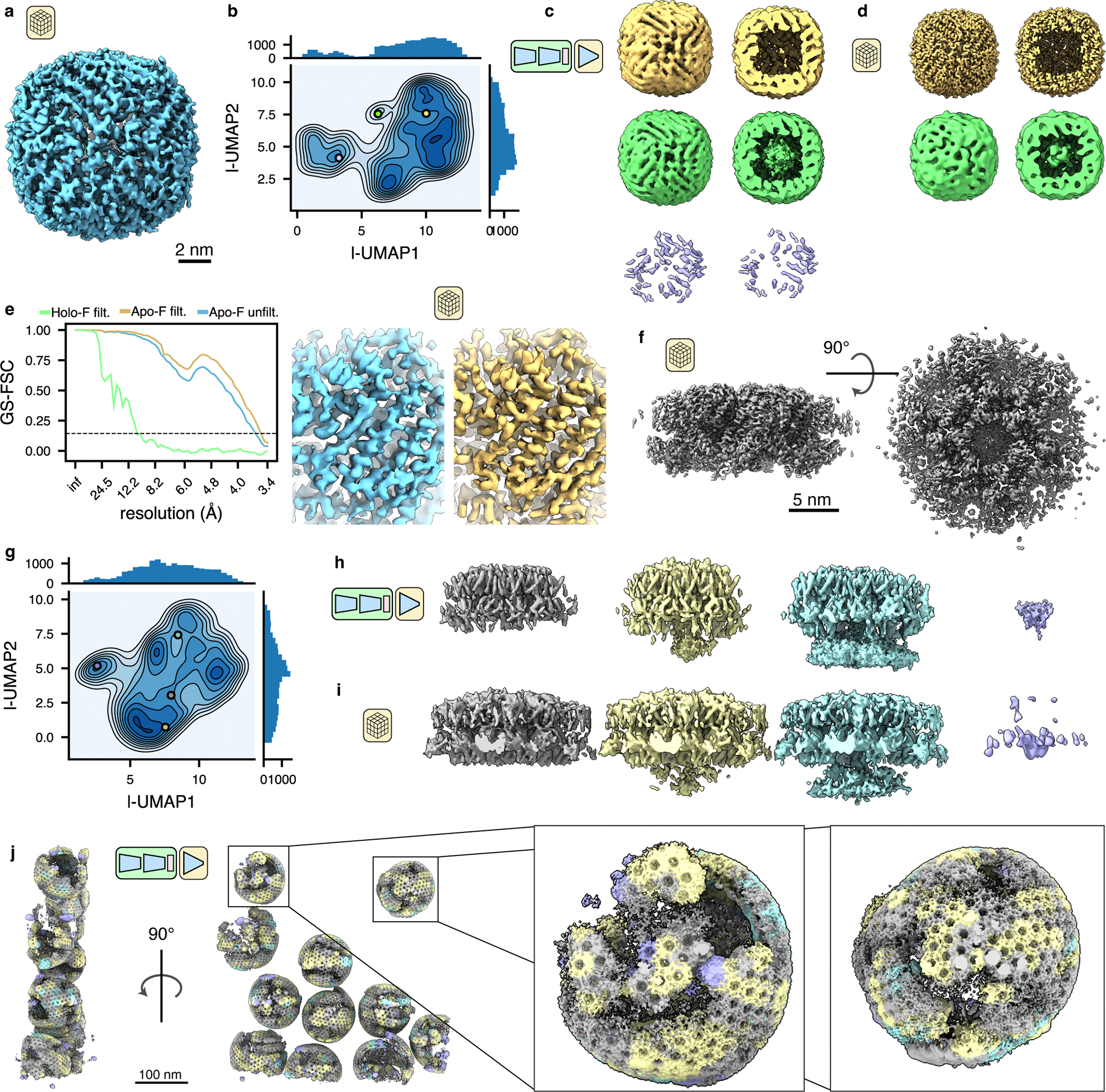
(a) Consensus STA apoferritin structure refined with C1 symmetry (EMPIAR-10491, n = 25,381 particles).

(b) UMAP dimensionality reduction of tomoDRGN latent encodings from training on apoferritin dataset.

(c) Three volumes generated from tomoDRGN latent encodings sampled as indicated in (b) and rendered in their entirety (left) or clipped in plane (right).

(d) Consensus STA reconstructions of apoferritin (n = 16,576 particles; top) and iron-loaded ferritin (n = 542 particles; bottom) from multi-species refinement in M with C1 symmetry using tomoDRGN’s particle classifications, rendered at constant isosurface as in (c).

(e) Gold standard FSC curves between half-maps from the final round of M refinement with C1 symmetry for unfiltered apoferritin particles (blue) and filtered apoferritin (yellow) and iron-loaded ferritin particles (green) (left). Example of local density quality before (blue) and after (yellow) tomoDRGN particle filtering of apoferritin particles (right).

(f) Consensus STA HIV gag structure refined with C1 symmetry (EMPIAR-10164, n=18,325 particles).

(g) UMAP dimensionality reduction of tomoDRGN latent encodings from training on HIV Gag dataset.

(h) Four illustrative volumes generated from tomoDRGN latent encodings sampled as indicated in (g). Note increasing density corresponding to the lower NC layer in the yellow and cyan maps relative to that in gray.

(i) Weighted back-projection reconstructions of isolated structural classes using tomoDRGN’s particle classifications (from left to right, n = 11,449 particles, 3,546 particles, 1,444 particles, and 1,674 particle), rendered at constant isosurface.

(j) An EMPIAR-10164 tomogram reconstructed with tomoDRGN. Volumes were generated for each Gag hexamer using tomoDRGN, colored as in (h, i), and positioned correspondingly in the source tomogram. Inset highlights two representative VLPs.

Another class of particles frequently analyzed by STA are those that assemble into massive structures using a large, semi-regular lattice. To assess tomoDRGN performance on such samples, we reprocessed the well-characterized immature HIV capsid dataset EMPIAR-10164 with a final symmetry relaxation step⁵¹, recapitulating clearly resolved CA-NTD and CA-CTD layers (Fig. 3f). Training a tomoDRGN model on this C1 dataset revealed a largely unfeatured latent space (Fig. 3g), with primary structural classes varying in their organization and extent of observed density of the NC layer underneath the CA layers (Fig. 3h,i). Application of MAVEn^8,9 using a mask encompassing the presumed location of the NC domain revealed a continuum of differentially occupied NC layers, consistent with extensive flexibility of this domain (Extended Data Fig. 3). At this resolution we could not clearly attribute the density seen in the NC layer to NC protein, nucleic acid used during sample reconstitution, or a combination thereof – a challenge that others have noted⁵². However, by reconstructing volumes corresponding to all particles with the trained tomoDRGN model and arranging them in the spatial context of the source tomogram, we observed groups of Gag hexamers with increased NC-layer density co-clustering within the VLPs (Fig. 3j). We postulate that this VLP-level patterning of NC-layer organization may reflect regions where the nucleic acid cargo is avidly and cooperatively bound by a local neighborhood of NC domains.

Uncovering structurally heterogeneous ribosomes in situ

As a final test, we applied tomoDRGN to the dataset EMPIAR-10499²⁷, using it to analyze heterogeneity among chloramphenicol-treated ribosomes imaged in the bacterium Mycoplasma pneumonaie. Following published STA methods²⁷, we reproduced a Nyquist-limited ~3.5 Å resolution reconstruction of the 70S ribosome (Fig. 4a–b). We subsequently extracted corresponding ribosome images from the aligned tilt micrographs and used this particle stack to train a homogeneous tomoDRGN model. The tomoDRGN-reconstructed volume recapitulated high-resolution features observed in the STA map including density for bulky side chains and for the bound chloramphenicol molecule (Fig. 4c–e), highlighting the tomoDRGN decoder network’s ability to accurately represent high-resolution structures in a dataset acquired in situ.

Figure 4: TomoDRGN resolves high resolution features from sub-tomograms collected in situ.

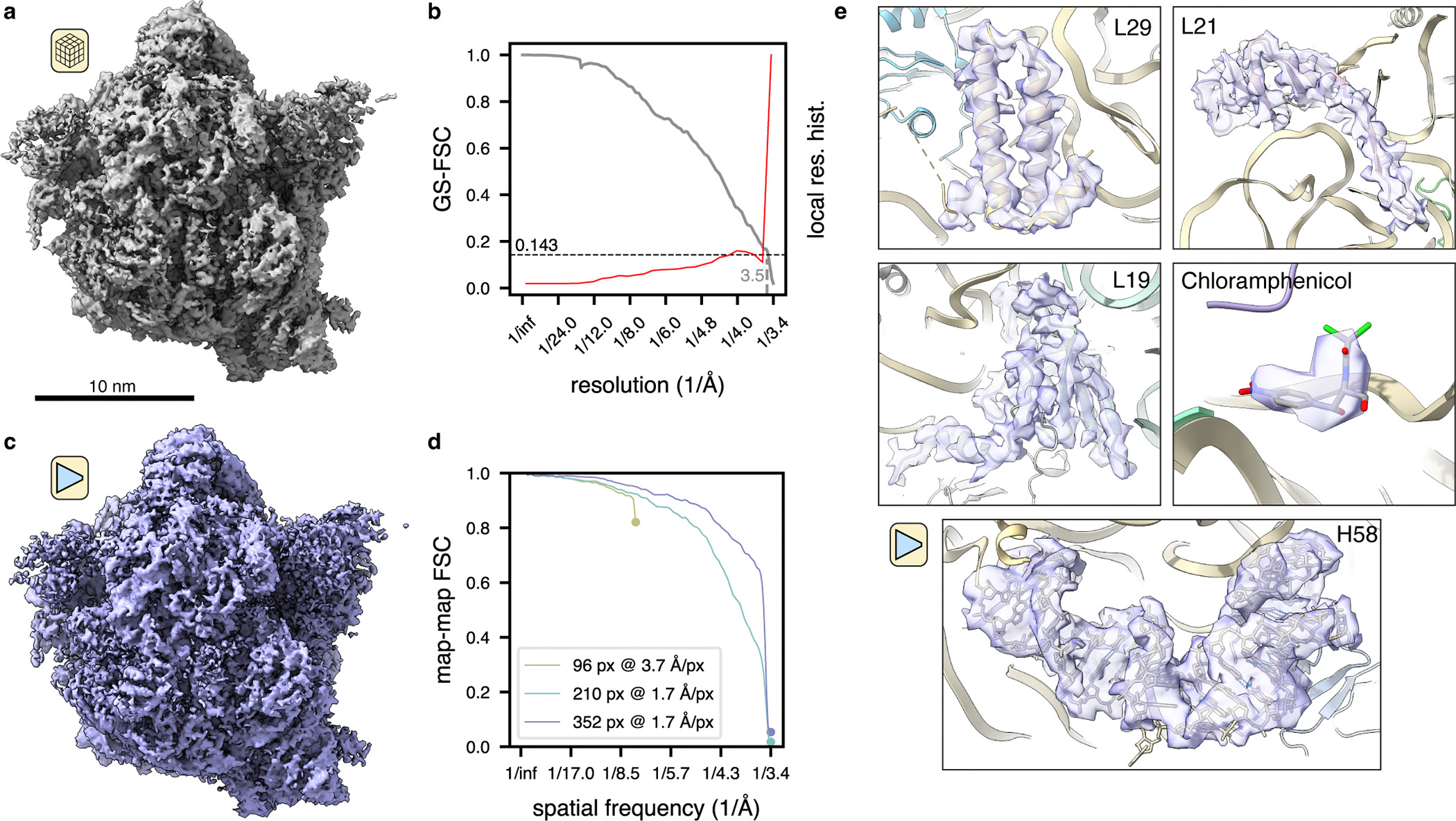
(a) M. pneumonaie ribosomal volume obtained from traditional STA processing (n=22,291 particles imaged in situ).

(b) Gold standard FSC curve between half-maps for the volume shown in (a). The second y-axis depicts a histogram of local resolution throughout the map.

(c) TomoDRGN homogeneous reconstruction of the particles used for the reconstruction in (a), lowpass filtered to 3.5Å.

(d) Map-to-map FSC of three tomoDRGN homogeneous reconstructions of the particle stack in (a) at indicated box and pixel sizes against corresponding STA volumes. Circles denote the Nyquist limit for each particle stack.

(e) Local density maps, lowpass filtered at 3.5Å, resulting from tomoDRGN homogeneous reconstruction in (c).

Encouraged by this result, we trained a heterogeneous tomoDRGN model on a down-sampled version of the particle stack and observed several distinct clusters in the resulting latent space (Fig. 5a, left). Generating volumes from these populated regions of latent space revealed that the majority of latent encodings corresponded to 70S ribosomes, as expected, while one subset corresponded to 50S ribosomal subunits, and another subset corresponded to apparent non-ribosomal particles (Fig. 5a, right). The non-ribosomal particles were further characterized by localizing them within each tomogram and providing them to RELION for ab initio reconstruction. Doing so revealed that these particles predominantly were false positive particle picks (Extended Data Fig. 4), highlighting tomoDRGN’s efficacy in sorting particles by structural heterogeneity even in situ. We additionally explored complementary filtering approaches that directly used the trained tomoDRGN model to generate unique volumes corresponding to every particle’s latent embedding. We then computed either each volume’s similarity to the 70S STA map (Fig. 5b) or performed principal component analysis (PCA) on the set of resulting volumes (Fig. 5c). These approaches produced results consistent with the clusters identified in latent space, highlighting the robustness of our initial latent-space-based filtering. As we expect the performance of these latent-space- and volume-based filtering approaches to vary on a per-dataset basis, users are encouraged to compare the efficacy of each approach on their own datasets.

Figure 5: TomoDRGN uncovers structural heterogeneity in ribosomes imaged in situ.

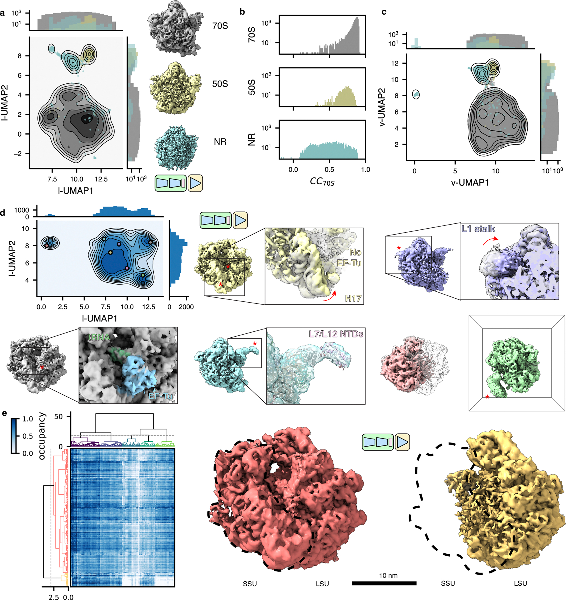
(a) UMAP of tomoDRGN latent embeddings (n=22,291 particles) shown as gray kernel density estimate (KDE), overlaid with scatter plot depicting latent embedding locations of large-ribosomal-subunit-only (yellow) or non-ribosomal particles (blue) identified via k=100 k-means classification of latent space and manual inspection of the 100 related volumes. Representative volumes generated from latent embeddings annotated as 70S, 50S, or non-ribosomal (NR) also depicted.

(b) Volumes (box=96 px) were generated from every particle’s latent embedding, and volumetric cross-correlation (CC) between the 70S STA map and these volumes was calculated. Histograms of CC are shown for volumes assigned as 70S (top), 50S (middle) and non-ribosomal (bottom) particles as in (a).

(c) Volumes from panel (b) were subjected to principal component analysis. UMAP dimensionality reduction of the first 128 principal components is plotted as a KDE with scatterplot corresponding to assignments of 70S, 50S, or non-ribosomal from (a) superimposed.

(d) UMAP of tomoDRGN latent embeddings (n=20,981; non-ribosomal particles excluded). Colored volumes sampled from correspondingly colored points on UMAP plot are shown with red asterisks and insets highlighting regions of notable structural variability. A transparent grey volume corresponding to a tomoDRGN reconstruction of a 70S•EF-Tu volume is provided for visual reference.

(e) MAVEn analysis⁹ of 500 volumes sampled from the tomoDRGN model in panel (d) plotted as a clustered heatmap with columns corresponding to proteins and rRNA structural elements (Ward-linkage, Euclidean-distance), and rows corresponding to the 500 sampled volumes (Ward-linkage, Correlation-distance). Distinct volume classes corresponding to 50S and 70S particles as identified by a row-wise threshold on this clustermap are also shown.

Guided by the latent embeddings, we next filtered out the non-ribosomal particles and used this “clean” subset to train a new heterogeneous tomoDRGN model. The resulting latent space and generated volumes revealed an array of structurally heterogeneous ribosomes (Fig. 5d). Prior analyses of this dataset have quantified translation cycle heterogeneity¹², with most (~75%) particles bearing tRNAs in the A- and P-sites (state 4), and a minority of particles with EF-Tu bound to the A-site with the E-site either occupied by tRNA (~10%; state 2e) or unoccupied (~10%; state 3). We observe broadly similar decoding and peptidyl transfer populations, with the majority (93%) of particles adopting state 4, and smaller populations in states 2e (0.5%) and state 3 (6%). Moreover, we observe additional conformational and compositional heterogeneity throughout the ribosome (Supplementary Video 2). For example, we observe conformational changes of 16S rRNA helix 17 consistent with SSU rotation for a set of particles lacking EF-Tu in the A-site. In other volumes, we observed pronounced motions of the L1 stalk. We also observed volumes with clear density for r-proteins L7/L12 in the expected 1:4 ratio of L10^CTD:L7^NTD/L12^NTD dimer of dimers, which was notable as this structural element is often unresolved in cryo-EM density maps^53,54, likely due to this stalk’s dynamic nature and L7/L12’s ability to exchange off of the particle during purification⁵⁵. Observing this structure highlighted tomoDRGN’s ability to identify low abundance classes and emphasized the promise of purification-free in situ structural analyses afforded by cryo-ET.

We next applied MAVEn^8,9, which has previously been used to systematically interrogate the structural heterogeneity of volume ensembles guided by atomic models. Here, we observe a broadly uniform distribution of occupancies for all queried structural elements (i.e., rRNA helices and r-proteins), with a notable exception of the 50S particle block, which lacks occupancy for any SSU structural elements, but is largely unfeatured in LSU structural elements (Fig. 5e), which led us to conclude that compositionally heterogeneous assembly intermediates are rare in this sample.

Exploring intermolecular heterogeneity in situ

A grand promise of in situ cryo-ET is its potential to structurally characterize interactions between individual macromolecular complexes and their local environment^27,56. We hypothesized that tomoDRGN might perform well in this regard as its VAE architecture has a significant capacity to learn heterogeneity from the provided images, independent of the images being tightly or loosely cropped to the particles of interest. Indeed, our initial analysis revealed volume classes containing apparent intermolecular density truncated by the extracted box borders (Fig. 5d). To test tomoDRGN’s ability to analyze inter-complex structural heterogeneity, we extracted each ribosomal particle at a larger physical box size, effectively surveying the molecular neighborhood of each ribosome in the imaged cell. Training a new “intermolecular” tomoDRGN model with these images revealed a similarly featured latent space with correspondingly diverse volumes (Fig. 6a). Many of the structures appeared to be disomes and trisomes, as previously reported²⁷, with measures of interparticle distance and angular distribution to each ribosome’s nearest neighbor consistent with this interpretation (Fig. 6b). Detailed inspection of these particles revealed instances of disomes bearing resolved mRNA density bridging the particles (Extended Data Figure 5, see Methods). Notably, in a subset of such cases, the ribosomes adopted a relative orientation stereotypical of stalled/collided particles, and each such particle bore additional density on the bridging mRNA at a location recently reported to be targeted by an RNase associated with the stalled ribosome rescue pathway⁵⁷.

Figure 6: TomoDRGN captures intermolecular heterogeneity in situ.

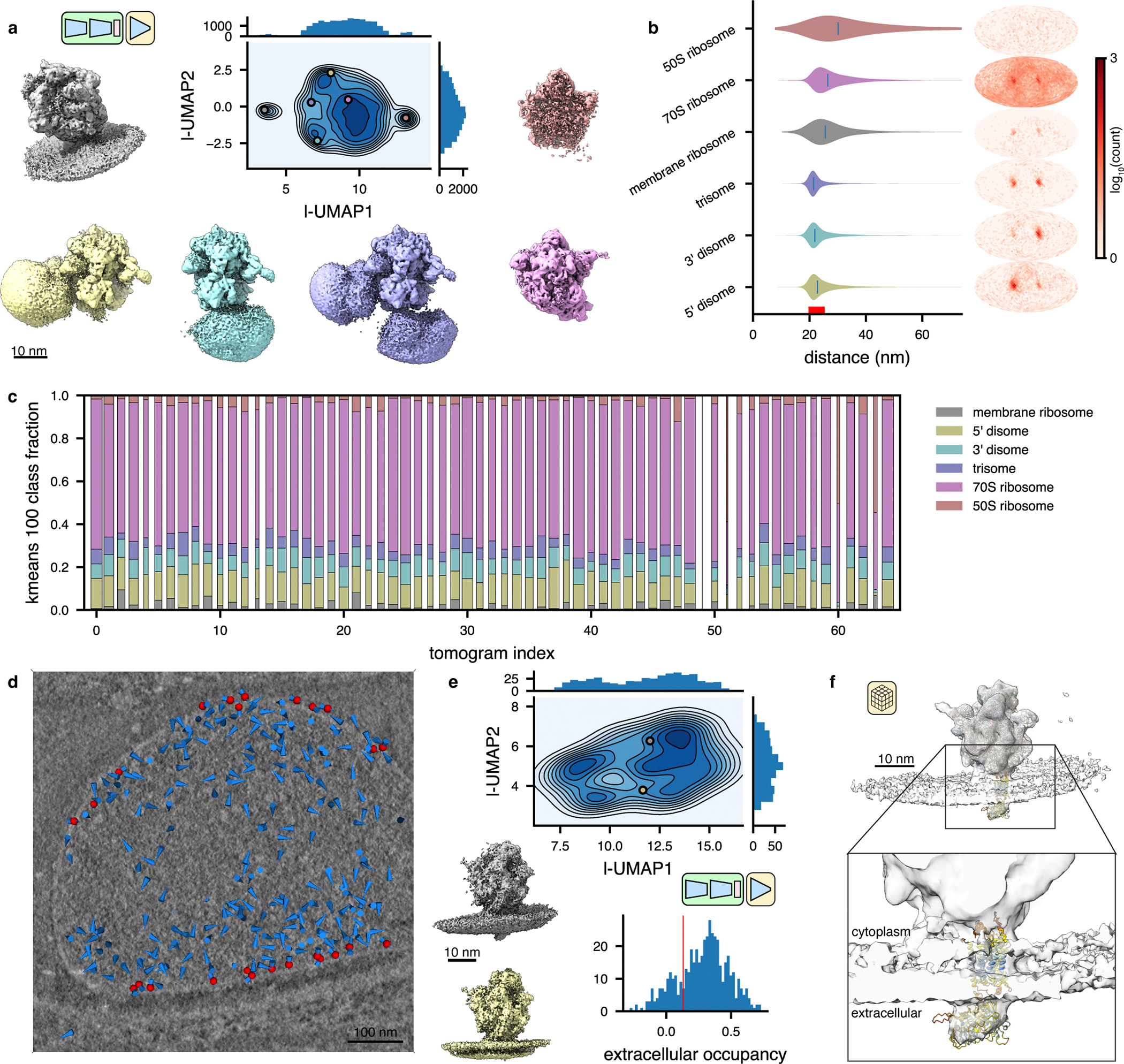
(a) UMAP of tomoDRGN latent embeddings (n=20,981 particles re-extracted with box size ~3x particle radius). Colored volumes sampled from correspondingly colored points in UMAP are shown.

(b) Violin plot of the distance from each particle in the indicated classes from panel (a) to its nearest neighbor ribosome. The right bound of the x-axis corresponds to the box diameter, and the red interval on the x-axis corresponds to typical inter-ribosome distances in a prokaryotic polysome. Mollweide projection histograms for each class highlighted in panel (a), showing directions to each ribosome’s nearest neighbor ribosome, following rotation to the consensus pose.

(c) Distribution of primary structural classes per tomogram. Column width is proportional to each tomogram’s particle count. Within a column, the height of each color is proportional to the population of that structural class within that tomogram. Classes are colored as in (a).

(d) Screenshot from tomoDRGN’s interactive tomogram viewer showing all ribosomes for a single tomogram (blue cones) with ribosomes corresponding to membrane-associated classes further annotated as red spheres.

(e) UMAP of tomoDRGN latent embeddings (n=482) of membrane-associated ribosomes. Colored volumes are sampled from correspondingly colored points in latent space. Relative occupancy of globular extracellular density (n=482) is plotted as a histogram with a red line noting manually assigned threshold defining particles bearing the extracellular density (n=380).

(f) STA reconstruction of membrane-associated ribosomes bearing extracellular density identified by tomoDRGN with docked atomic model of Mycoplasma pneumoniae SecDF predicted using Alphafold (AF: A0A0H3DPH3).

When analyzing particles using the intermolecular tomoDRGN model, we additionally observed a ribosome structure previously unreported in this dataset with additional density corresponding to a lipid bilayer (Fig. 6a). We mapped this set of apparently membrane-associated ribosomes to their original tomograms and observed that they exclusively corresponded to particles at the cell’s surface (Fig. 6d). To identify residual heterogeneity within this group, we trained a new tomoDRGN model on this particle subset and observed a relatively unfeatured latent space, with the majority (~80%, as quantified by MAVEn) of sampled volumes bearing a flexible extracellular density protruding from the membrane (Fig. 6e). Notably, we observed significant motion between the ribosome and the adjacent membrane, indicating that the ribosome was not held in rigid alignment with the membrane and holotranslocon during translocation (Supplementary Video 3). Traditional STA on this extracellular-positive subpopulation of ribosomes further resolved the extracellular density, as well as smaller arches of density connecting the ribosome to the membrane (Fig. 6f, Extended Data Fig. 6c). Rigid body docking using atomic models of likely transmembrane protein complexes into this density supported the presence of SecDF, a subcomplex of the Sec holotranslocon with a relatively large extracellular globular domain encoded by M. pneumoniae (Fig. 6f). This result highlighted the efficacy of tomoDRGN’s iterative particle curation and refinement approach in unveiling new structures buried in highly heterogeneous in situ datasets.

DISCUSSION

In this work, we introduce tomoDRGN, which, to our knowledge, is the first neural network framework capable of simultaneously modeling compositional and conformational heterogeneity from cryo-ET data on a per-particle basis. TomoDRGN achieves this using a bespoke deep-learning architecture and numerous accelerations designed to exploit redundancies inherent to cryo-ET data collection. We note that several analyses explored in this manuscript were originally tested with cryoDRGN⁴. However, cryoDRGN ultimately did not match tomoDRGN’s performance on cryo-ET data as it incorrectly classified simulated data, predominantly learned non-biological structural heterogeneity, and produced highly variable latent embeddings and volumes for different tilt images of the same particle (Extended Data Fig. 7–9), ultimately motivating development of tomoDRGN. We note that an alternative approach of mapping single sub-tomogram volumes to single latent coordinates would theoretically function within the cryoDRGN framework but would: 1) be less computationally tractable due to cubic scaling of the number of voxel coordinates to be evaluated per particle; and 2) may be predisposed towards learning heterogeneity driven by missing wedge artifacts common to sub-tomogram volumes. Finally, during revision of this manuscript, a related approach that uses a subset of the low-tilt images within the cryoDRGN framework was proposed⁵⁸. We expect that this method will perform similarly to tomoDRGN when analyzing ribosomes, which, because of their high abundance and lack of preferred orientation, do not require high-tilt angle information to generate isotropic maps.

TomoDRGN’s data inputs, as projection images with associated pose and CTF parameters, pose two potential limitations. First, inaccuracies in pose estimation during upstream STA processing could limit tomoDRGN reconstruction and classification accuracy. We explored this effect on our EMPIAR-10499 unfiltered ribosomes by treating the poses derived through STA as “ground truth” and progressively perturbing each particle’s rotation and translation to greater extents. In homogeneous reconstructions, we observed that tomoDRGN’s decoder-only network produced nearly equivalent reconstructions up to around 0.8° rotation and 0.8Å shift perturbation, with greater perturbations producing progressively worse reconstructions (Extended Data Fig. 10a–b). Heterogeneous tomoDRGN models captured meaningful structural heterogeneity even up to 1.6° and 1.6Å perturbation, particularly through principal component analysis of tomoDRGN-generated volume ensembles (Extended Data Fig. 10c–e). The second limitation of tomoDRGN’s approach derives from the possibility for other “background” signals that superimpose with a particle’s projection at particular stage-tilt angles, potentially misdirecting the latent encoding for this particle. We expect such superimposition is common, particularly for in situ samples. However, tomoDRGN’s random tilt subsampling per particle decreases the likelihood that multiple images bearing the same confounding signal will be sampled and encoded in the same pass. Additionally, tomoDRGN’s pooling of intermediate latent encodings in Encoder B adds further robustness against a minor fraction of such images. Indeed, we observed that volumes of a particular class co-localize in the structured latent space and produce similar volumes, even for in situ data (Fig. 5a–c), and we note that such robustness that has been similarly observed in EMAN-2’s use of 2D tilt images for STA refinement²⁸.

An additional consideration for prospective users is the types of particles to which tomoDRGN is best suited. As with most SPA and STA tools, we expect tomoDRGN will perfom best with large, abundant particles. The analyses of experimental data presented here have typically used between 15,000 – 25,000 particles of mass ranging from ~200 kDa to 2.5 MDa. In a notable exception (Fig. 6e) however, we demonstrated that as few as 482 ribosomes were sufficient to train de novo a tomoDRGN model capable of distinguishing the presence or absence of SecDF. While most SPA and STA tools can employ symmetry-based averaging to further increase the effective particle count, tomoDRGN’s decoder module is best suited to C1-symmetric pose distributions, and we therefore recommend symmetry relaxation or expansion of symmetric complexes prior to tomoDRGN analysis. In all demonstrated analyses, the input particles were aligned by STA without imposed symmetry to resolutions of ~4 Å; and while such resolutions will aid users gaining the greatest insights from tomoDRGN, we also often use tomoDRGN significantly earlier in data processing to aid upstream particle filtering and guide general particle classification.

Other tools to explore conformational heterogeneity from a cryo-ET dataset have been recently introduced^17,29,33,34. However, they each rely on some degree of imposed prior structural knowledge, either in the form of “mass conservation” to describe continuous changes from a consensus structure, which is often derived from a provided atomic model^33,34; assumptions of linear relationships between structures²⁹; or the assertion that a small number of discrete structures exist¹⁷. In contrast, tomoDRGN’s approach provides a greater degree of generality that we have found enables a largely unsupervised analysis of datasets with highly complex combinations of compositional and continuous conformational heterogeneity. Given the extent of structural heterogeneity observed with cryoDRGN in single particle datasets using purified samples^59,60, we expect tomoDRGN to uncover similar structural variation within a rapidly expanding set of samples imaged in situ with cryo-ET. For tomoDRGN, as with all of these heterogeneity analysis tools, we emphasize that observed structural variation should be validated, including by reconstruction of the particles bearing the structural feature of interest by an alternative approach (e.g. weighted back-projection), by comparison with known biology, and ideally, by orthogonal experimental approaches.

As is true with other STA processing pipelines, we expect that using tomoDRGN to reanalyze particle stacks at different spatial scales (i.e., different real space box sizes) will prove useful in correlating intramolecular structural changes with structural variability areas adjacent to the particle (Extended Data Fig. 5). Of particular note, leveraging tomoDRGN’s expressivity to generate a unique 3-D volume corresponding to each particle’s latent embedding enables users to populate low SNR cellular tomograms with individualized density maps at approximately nanometer resolution and explore the resultant spatial distributions of heterogeneous structures. Here, we used this approach to resolve meso-scale patterning of NC-layer organization among Gag hexamers (Fig. 3j), and to directly identify disomes in situ (Extended Data Fig. 5a–b). By combining multi-scale analysis and tomoDRGN’s per-particle volume generation, we were able to further identify distinct structural classes of these disomes, including direct visualization of mRNA threading within and between individualized monosome structures (Extended Data Fig. 5c–f, Supplementary Video 4).

Finally, the analyses enabled by tomoDRGN are inherently iterable. Our initial tomoDRGN analysis of EMPIAR-10499 revealed a population of non-ribosomal particles that we had failed to filter with traditional classification-based approaches. Excluding such particles and retraining at multiple spatial scales resolved intra- and inter-molecular structural heterogeneity, and retraining exclusively on a subset of membrane-associated ribosomes identified extracellular density that likely corresponded to the SecDF subcomplex. Given that tomoDRGN has the potential to identify many such distinct classes, we encourage users to embrace this branching and iterative approach. Some recently introduced software packages^27,61 explicitly support such “molecular sociology” where co-refinement of multiple distinct structures derived from a common data source globally enhances the quality of individual maps. We anticipate tomoDRGN will form a virtuous cycle when interfacing with such software.

METHODS

TomoDRGN design and software implementation

General architecture

TomoDRGN is forked from cryoDRGN. Thus we summarize the core aspects of the method here, and direct readers to related cryoDRGN publications for further details^4,8,39,40. Briefly, tomoDRGN is a variational autoencoder (VAE) with encoder and decoder networks comprised of multi-layer perceptrons (MLPs). TomoDRGN’s encoder learns a function ($E$) to map a set of $j$ tilt images (size $D\times D$ pixels) of particle $i$ to a low dimensional latent encoding $z_i$ of dimension $z$; that is, $E:{\mathbb{R}}^{j\mathrm{*}D\mathrm{*}D}\to {\mathbb{R}}^z$. The encoder MLP comprises two sub-networks that process $j$ tilt images for each particle as follows. First, the 2-D Hartley transform of each tilt image is passed separately through encoder A to produce a set of $j$ intermediate encodings. These $j$ intermediate encodings are then pooled and passed together through encoder B to output the particle’s final latent embedding $z_i$. The pooling step concatenates intermediate encodings along the tilt image axis by default, but also supports operations such as max and mean, which are inherently permutation-invariant. All experiments presented here concatenate the intermediate encodings.

TomoDRGN’s decoder follows from that of cryoDRGN⁴, and uses a Gaussian featurization scheme for positional encoding in Fourier space ⁶² as follows. Spatial coordinates are normalized to span [−0.5, 0.5] in each dimension, and a (fixed) positional encoder transforms each spatial coordinate to a basis set of D sinusoids with frequencies sampled from a scaled standard normal $feat\_sigma\times 𝒩\left(\mathrm{0,1}\right)$ for each spatial coordinate axis, where D is the box size of an input image, and feat_sigma is set to 0.5. These positionally encoded coordinates, concatenated with the z-D latent coordinate, are then passed to the decoder; that is, in totality, $D:{\mathbb{R}}^{3+z}\to \mathbb{R}$. Unless otherwise specified, models were trained for 50 epochs with batch size 1 (particle), using the AdamW optimizer with learning rate of 0.0002, and weight decay of 0.

Training system

Input images are modeled as 2-D projections of 3-D volumes, convolved by the contrast transfer function (CTF), with externally-provided rotation, translation, and CTF parameters. Heterogeneity among volumes is modeled via a continuous latent space sampled by a latent variable z per particle. The latent encoding for a given image $X$ is taken as the maximum a posteriori of a Gaussian distribution parameterized by outputs from the encoder network, ${\mu }_{z|X}$ and ${\mathrm{{\rm X}}}_{z|X}$, whereas the prior on the latent distribution is a standard normal distribution $𝒩\left(0,\mathit{I}\right)$. Thus, the variational encoder $q_{\xi }\left(z|X\right)$ produces a variational approximation of the true posterior $p\left(z|X\right)$. The coordinate-based decoder models structures in reciprocal space: given a spatial frequency $k\in {\mathbb{R}}^3$ and a latent variable $z$, the decoder predicts the corresponding voxel intensity as $p_{\theta }\left(V\right|k,z)$.

Applying the Fourier Slice Theorem⁶³, 3-D Fourier coordinates corresponding to 2-D projection image $X_i$ are derived by rotating a 2-D lattice by the orientation of the volume $V_i$ during imaging. Given a fixed latent coordinate sampled from $q_{\xi }\left(z_i|X_i\right)$ and the posed coordinate lattice, the reciprocal space image is reconstructed pixel-by-pixel via the decoder $p_{\theta }\left(V\right|k,z_i)$. The reconstructed image is then translated in-plane and multiplied by the CTF. The negative log-likelihood of the image is then computed as the mean squared error between the input and reconstructed image. The optimization function is the sum of the image reconstruction error and the KL divergence (KLD) of the latent encoding:

$$ℒ\left(X;\xi ,\mathrm{\Theta }\right)=E_{q_{\xi }\left(z|X\right)}\left(\log p\left(X|z\right)\right)-\beta KL(q_{\xi }(z|X)||p\left(z\right))$$

In this equation, the regularizing KLD term is weighted by $\beta ,$ which is set to $\frac{1}{|z|*t*D^2}$, where D is the box size, t is the number of tilts, and $|z|$ is the dimensionality of the latent space.

Lattice masking and reconstruction weighting

Critical dose is calculated for each spatial frequency using an empirical exposure-dependent amplitude attenuation curve derived for cryo-EM data ⁴³. The optimal dose is approximated to $2.51284\times criticaldose$ as in the original study^43,45. Spatial frequencies (coordinates) of a tilt image exceeding the corresponding optimal doses are excluded from decoder network evaluation and loss calculation by a lattice mask during network training. Following error calculation of the input image against the reconstructed and CTF-weighted voxels, the squared differences are weighted (1) per-frequency by the exposure dependent amplitude attenuation curve (a function of tilt image index and spatial frequency), and (2) globally by the cosine of the stage tilt angle in radians (a function of tilt image index). This weighted reconstruction error is backpropagated accordingly.

Random tilt sampling

During dataset initialization, the number of tilt images per particle is parsed via the rlnGroupName star file column using the syntax in Warp/M of tomogramID_particleID. The minimal number of tilt images present for any particle (n) is then stored as the number of images to be sampled from each particle during network training and evaluation (this value also sets the input dimensionality of encoder B when using concatenation pooling). The value n is reported by tomoDRGN during training initialization, and we recommend users to exclude tilt series where this value is below 11. By default, sampling is performed randomly without replacement per-particle, and the subset and ordering of sampled tilts is updated each time a particle is retrieved during training or evaluation.

Simulated dataset generation

Cryo-ET data simulation was performed using scripts in the cryoSRPNT (cryo-EM Simulation of Realistic Particles via Noise Terms) GitHub repository. Source data for the bacterial ribosome LSU dataset was obtained as density maps of four assembly states of the bacterial 50S ribosome (classes B - E) (EMD-8440, EMD-8441, EMD-8445, and EMD-8450, respectively)⁴⁸. For the yeast ATP synthase dataset, atomic models (7TK6, 7TK7, 7TK8, 7TK9, 7TKA, 7TKB, 7TKC, 7TKD) were obtained from the PDB. ChimeraX’s morph functionality was used to interpolate between each state, resulting in 400 atomic models smoothly sampling the conformational changes underlying the experimental model ensemble. Each atomic model was then converted to a volume using ChimeraX’s molmap functionality at 3Å/px sampling and resolution of 6Å.

The project3d.py script was used to create noiseless projections of each volume as follows. For the LSU dataset, 5,000 random particle poses were sampled over SO(3) for each volume; for the ATP synthase dataset, this number was 50 poses per volume. Thus, each dataset totals 20,000 uniquely posed particles. Each posed particle was then rotated following a dose-symmetric tilt series scheme from 0° to +/−60° with 3° steps in groups of 2 over 41 tilts and each tilted volume was projected along the z-axis to create noiseless images.

The acn.py script was used to corrupt the noiseless projections using a standard cryo-EM image formation model⁴⁷ augmented by tilt-series specific subroutines as follows. First, noiseless projections were Fourier-transformed, dose-weighted following an empirical exposure dependent amplitude attenuation curve at 3 e⁻/Ų/tilt to simulate SNR decrease due to radiation damage⁴³, and inverse Fourier-transformed. Structural noise was added with an SNR of 1.4, and particles were then weighted by cosine(tilt_angle) to simulate SNR decrease due to increased sample thickness. Projections were then convolved with the 2-D CTF with defocus values sampled from a mixture of Gaussian-distributed defoci with means between −1.5 μm to −3.5 μm in 0.5 μm steps and a standard deviation of 0.3 μm. Other CTF parameters included no astigmatism, 300 kV accelerating voltage, 2.7 mm spherical aberration, 0.1 amplitude contrast ratio, and 0° phase shift. Finally, shot noise was added with a SNR of 0.1, for a final SNR of 0.05, a level consistent with other simulation approaches used in the field^{4,20,22,64,65}. For the LSU dataset, particle stacks of each class were Fourier cropped to box sizes of 256px (3Å/px; bin1), 128px (bin2), and 64px (bin4). For the ATP synthase dataset, only the original 114px (3Å/px) dataset was generated.

TomoDRGN network training and analysis of simulated LSU dataset

TomoDRGN homogeneous network training was performed on the 5,000 simulated class E particles. TomoDRGN heterogeneous network training was performed on all 20,000 simulated particles from classes B-E. Unless otherwise specified, figures illustrate results on the bin2 datasets, with network architectures summarized as nodes_per_layer x layers as follows: 128×3 (encoder A), 128×3 (encoder B), and 256×3 (decoder). The dimensionality of the A-B intermediate encoding was 32 and that of the final latent encoding was 128. Each model was trained using dose and tilt loss weighting, dose frequency masking, and random tilt sampling, unless specified otherwise. Classification was performed directly on the latent embeddings with k=4 k-means clustering as implemented in scikit-learn. The dataset’s latent value nearest each k-means cluster center was used to generate a 3-D volume representative of that cluster.

TomoDRGN network training and analysis of simulated ATP synthase dataset

TomoDRGN heterogeneous network training was performed on all 20,000 simulated ATP synthase particles. The network architecture, summarized as nodes_per_layer x layers, was as follows: 256×3 (encoder A), 256×3 (encoder B), and 256×3 (decoder). The dimensionality of the intermediate encoding was 128 and that of the final latent encoding was 128. The model was trained using dose and tilt loss weighting, dose frequency masking, and random tilt sampling for 50 epochs. Following model training, 500 latent embeddings were sampled via k=500 k-means classification; volumes were generated at each sampled embedding using the trained tomoDRGN model and subjected to unmasked real-space PCA.

Sub-tomogram averaging of EMPIAR-10491 apoferritin

Raw tilt movie data was downloaded from EMPIAR-10491. Movies were aligned and initial CTF estimation was performed in Warp⁶⁶ as previously reported²⁷ modified by binning movies to 1.668 Å/px in Warp. Automated patch-based tilt series alignment was performed using Aretomo v1.3.4⁶⁷. Alignment parameters were then used to generate tomograms at 10 Å/px in Warp. Template matching was performed in Warp using a 40 Å lowpass filtered apoferritin volume generated from manually picked particles, keeping particles with a minimum separation of 20 Å. The top 700 of particles by figure-of-merit per tomogram were kept (25,900 particles). Sub-tomograms were extracted in Warp at 1.668 Å/px. Ab initio model generation and 3-D refinement were performed in RELION 3.1.3¹⁷ with octahedral symmetry applied, resulting in a reconstruction of ~3.9 Å resolution. Particles were deduplicated with a cutoff distance of 50Å (removing 519 particles). RELION 3-D classification was performed with pose alignment in C1 or O symmetry with varying numbers of classes, but no non-apoferritin classes were detected for removal. All particles were imported into M to improve tomogram-level parameters while taking advantage of octahedral symmetry during iterative refinement of particle poses, tilt geometry, image warp, volume warp, and defocus, resulting in a reconstruction of resolution ~3.4Å. Sub-tomograms were re-extracted in M at 1.668Å/px for further RELION 3-D refinement in C1, which resulted in a reconstruction of resolution 4.6 Å. These particles were imported to M in C1 and subjected to the same iterative M refinements to produce a final 3.6Å resolution map. Particles were then exported as image series sub-tomograms from M at 1.668Å/px and box size 132px for tomoDRGN training. Particles were also exported as volume series sub-tomograms using M at 132px 1.668Å/px for generation of requisite metadata for mapping particles to tomogram-contextualized locations and particle re-extraction and filtering in M. Note that for this dataset, this metadata was used only for particle re-extraction and filtering.

TomoDRGN network training on EMPIAR-10491 apoferritin

TomoDRGN heterogeneous network training was performed on all 25,381 apoferritin particles. The network architecture was as follows: 256×3 (encoder A), 256×3 (encoder B), and 256×3 (decoder). The dimensionality of the intermediate encoding was 128 and that of the final latent encoding was 128. The model was trained using dose and tilt loss weighting, dose frequency masking, and random tilt sampling for 15 epochs. Following model training, 100 latent embeddings were sampled via k=100 k-means classification; volumes were generated at each sampled embedding using the trained tomoDRGN model and visually classified into apoferritin, holoferritin, or junk particles. A randomly selected representative of each class is shown in Figure 3c. The M volume-series subtomogram star file was filtered according to the tomoDRGN classification indices for new multi-species population creation and further iterative C1 refinement in M.

Sub-tomogram averaging of EMPIAR-10164 HIV Gag capsid CA-layer

Processing broadly followed the walkthrough guide provided at teamtomo.org. Raw tilt movie data for the standard subset of 5 tilt series used in benchmarking cryo-ET software was downloaded from EMPIAR-10164. Movies were aligned and initial CTF estimation was performed in Warp⁶⁶. Automated fiducial-based tilt series alignment was performed using dautoalign4warp⁶⁸ within the Dynamo package running in a Matlab environment¹⁹. Tomograms were reconstructed in Warp at 10Å/px. Dynamo was used to oversample manually annotated spherical lattices corresponding to each VLP, and subsequent spherical lattice geometry filtering was applied to filter particles. An initial model was generated and refined in Dynamo, and duplicate particles from oversampling were removed (keeping n = 18,325 particles). Sub-tomograms were extracted in Warp at 5Å/px for 3-D refinement performed in RELION 3.1¹⁷ with C6 symmetry applied. Sub-tomogram extraction and RELION refinement was repeated at 1.6 Å/px with C6 symmetry (~4.2Å resolution achieved). All particles were imported into M to improve tomogram-level parameters while taking advantage of C6 symmetry during iterative refinement of particle poses, tilt geometry, image warp, volume warp, defocus, Zernike orders 2–5, and tilt movies (~3.3Å resolution achieved). Sub-tomograms were re-extracted in M at 1.6 Å/px for further RELION 3-D refinement in C1 via symmetry relaxation (~4.8Å resolution achieved). The final 18,325 particles were imported to M and subjected to the same iterative M refinements to produce a 3.9 Å map. Particles were then exported as image series sub-tomograms from M at 1.6Å/px and box size 128 px for tomoDRGN training. Particles were also exported as volume series sub-tomograms using M at 64 px 3.2 Å/px for generation of requisite metadata for mapping particles to tomogram-contextualized locations and particle re-extraction and filtering in M.

TomoDRGN network training on EMPIAR-10164 HIV Gag capsid CA-layer

TomoDRGN heterogeneous network training was performed on all 18,325 Gag hexamers. The network architecture was as follows: 256×3 (encoder A), 256×3 (encoder B), and 256×3 (decoder). The dimensionality of the intermediate encoding was 128 and that of the final latent encoding was 128. The model was trained using dose and tilt loss weighting, dose frequency masking, and random tilt sampling for 25 epochs. Following model training, 100 latent embeddings were sampled via k=100 k-means classification; volumes were generated at each sampled embedding using the trained tomoDRGN model and visually classified into Gag with only CA-layer resolved, the same with moderate NC-layer density, the same with larger NC-layer density, or junk particles. A randomly selected representative of each class is shown in Figure 3h. Weighted back-projection and lowpass-filtering of the particles image-series subtomograms was performed in tomoDRGN using particle classifications derived from the tomoDRGN k=100 classification labels.

Sub-tomogram averaging of EMPIAR-10499 ribosomes

Raw tilt movie data was downloaded from EMPIAR-10499. Movies were aligned and initial CTF estimation was performed in Warp ⁶⁶ as previously reported²⁷. Automated fiducial-based tilt series alignment was performed using dautoalign4warp⁶⁸ within the Dynamo package running in a Matlab environment¹⁹. Alignment parameters were then used to generate tomograms at 10 Å/px in Warp. Template matching was performed in Warp using a 40 Å lowpass filtered ribosome volume generated from manually picked particles, keeping particles with a minimum separation of 80 Å (974,804 particles). The top 3% of particles by figure-of-merit across all tomograms were kept (29,245 particles). Sub-tomograms were extracted in Warp at 10 Å/px. Ab initio model generation and 3-D refinement were performed in RELION 3.1¹⁷ resulting in a density map with Nyquist-limited resolution. Sub-tomograms were re-extracted in Warp at 4 Å/px for further RELION 3-D refinement and 3-D classification with k=4 classes to remove false positive particle picks. The remaining 22,291 ribosomal particles were refined to a resolution of ~8.1 Å. Between each round of refinement and classification, particles were deduplicated in RELION with a cutoff distance of 80Å (removing a total of 360 particles throughout processing). The final 22,291 particles were imported to M and processed to produce a ~3.5 Å resolution map as reported previously²⁷. Particles were then exported as image series sub-tomograms from M at several pixel and box sizes for tomoDRGN training, including three “single ribosome diameter” scales: 96 px at 3.71 Å/px, 210 px at 1.71 Å/px, 352 px at 1.71 Å/px; and one “multiple ribosome diameter” scale: 200 px at 3.71 Å/px. Particles were also exported as volume series sub-tomograms using M at 64 px 6 Å/px and 192 px 4 Å/px for validation of tomoDRGN heterogeneity analysis with traditional STA tools and for generation of requisite metadata for mapping particles to tomogram-contextualized locations in the tomoDRGN analysis Jupyter notebook.

TomoDRGN network training on EMPIAR-10499 ribosomes

TomoDRGN homogeneous network training was performed on the 22,291 image series particles extracted at each of the “single ribosome diameter” image series sub-tomograms described above, or on select subsets at 96 px at 3.71 Å/px for homogeneously reconstructing subsets of the heterogeneous population. Unless specified otherwise, the network architecture was 512×3 (decoder). Each model was trained using dose and tilt loss weighting, dose frequency masking, and random tilt sampling.

TomoDRGN heterogeneous network training was performed on the same stack of 22,291 image series particles at box 96 px and 3.71 Å/px. Unless specified otherwise, the network architecture was 256×3 (encoder A), 256×3 (encoder B), and 256×3 (decoder) with the dimensionality of the intermediate encoding set to 128, and that of the final latent encoding set to 128. Each model was trained using dose and tilt loss weighting, dose frequency masking, and random tilt sampling. Classification was performed directly on the latent embeddings with either k=20 (used for general visualization) or k=100 (used for detailed visualization and particle filtering) k-means clustering as above. The dataset’s latent value nearest each k-means cluster center was used to generate a 3-D volume representative of that cluster. Following exclusion of 1,310 non-ribosomal particles by separation of such volumes from k-100 classification, the remaining 20,981 particles were used to train new tomoDRGN models at box sizes of 96 and 200 px with 3.71 Å/px sampling. Membrane associated ribosomes (482) identified by k-100 classification of the 200 px trained dataset were further isolated to train a new tomoDRGN model with the parameters noted as above.

Visualization and validation

Python scripts

A number of Python scripts were generated to quantify various properties of tomoDRGN outputs. Classification accuracy of tomoDRGN latent encodings learned for simulated datasets was evaluated by generating a confusion matrix (Fig. 2e). Classification reproducibility was evaluated for 100 randomly initialized classifications by calculating the Adjusted Rand Index (ARI)⁶⁹ (Extended Data Fig. 7f). The ARI measures a label-permutation-invariant similarity between two sets of clusterings and scales from 0 (random labeling) to 1 (identical labeling). Here, we used ARI to measure the similarity between the tomoDRGN or cryoDRGN latent clusters and the ground truth class labels.

Volumes generated by tomoDRGN were analyzed by either real space map-map correlation coefficient (CC)⁷⁰, or map-map Fourier shell correlation (FSC) metrics. Map-map FSC was used to assess the accuracy of a tomoDRGN homogeneous network reconstruction to a reference volume, whereas map-map CC was used to validate consistency of volume ensembles produced by tomoDRGN heterogeneous networks, either to themselves or to a reference volume. Calculations were performed using Python scripts available within the tomoDRGN software. Before calculating map-map FSC curves, a soft mask was calculated and applied in Real space. Masks were defined by binarizing the map at ½ of the 99^th voxel intensity percentile, dilating the mask by 3 px, and softening the mask using a falling cosine edge applied over 10 px.

Heterogeneity of a set of EMPIAR-10499 pre-filtered ribosome volumes generated by tomoDRGN was quantified by generating all volumes from the final epoch of training’s latent values and either (1) calculating the map-map CC to the STA 70S map for each tomoDRGN volume (Fig. 5b), or (2) performing principal component analysis on the array of all volume’s voxels (shape $n_{volumes}\times D^3$) followed by UMAP dimensionality reduction of the first 128 principal components (Fig. 5c).

Finally, Python scripts were used to identify each particle’s nearest neighbor in each tomogram, calculate the distance to the nearest neighbor, and calculate the angle to the nearest neighbor after rotating to the STA consensus reference frame (Fig. 6c).

Volume subset validation for EMPIAR-10499 ribosomes

Subsets of the EMPIAR-10499 ribosomes were identified by tomoDRGN as non-ribosomal (n=1,310), 50S (n=852), 70S (n=20,129), or membrane-associated (n=482). Non-ribosomal particles were reprocessed in RELION 3.1 using ab initio volume generation with k=5 volume classes and all other parameters at their defaults. The 50S, 70S, and membrane-associated ribosome populations were reprocessed in RELION 3.1 using 3-D refinement against a corresponding real-space cropped 70S volume lowpass filtered to 60 Å. The same three particle subsets were also used to train tomoDRGN homogeneous networks as an additional validation, with identical training parameters to the full particle stack training detailed above.

Visualization of tomoDRGN volumes in situ

The subtomo2chimerax script (https://zenodo.org/record/6820119) was adapted to handle tomoDRGN’s unique sub-tomogram volumes per particle and is implemented in tomoDRGN. This script places each particle’s volume at its source location and orientation in the tomogram context using ChimeraX for visualization^71,72. All volumes corresponding to EMPIAR-10164 tomogram 43 were generated by tomoDRGN at box size 32px and 6.4Å/px using latent coordinates from the tomoDRGN model in Fig. 3g, and placed in tomogram 43 with coordinate and angle values extracted from the STA refinement in M. Similarly, all volumes corresponding to EMPIAR-10499 tomogram 00256 were generated by tomoDRGN at various box and pixel sizes using corresponding latent coordinates from tomoDRGN models in Fig. 5d and Fig. 6a, and placed in tomogram 00256 with coordinate and angle values extracted from the STA refinement in M.

Atomic model-guided analyses of EMPIAR-10499 ribosomes

To aid interpretation of tomoDRGN density maps, atomic models of the 70S ribosome (7PHA, 7PHB, and 4V89 which highlighted the L7/L12 dimers) were docked into density maps as rigid bodies using ChimeraX. The rRNA of 7PHB was segmented into distinct chains corresponding to rRNA helices⁷³ following the MAVEn protocol⁸ for model-based analysis of volume ensembles (https://github.com/lkinman/MAVEn). Translation states populations were identified by generating maps from the 10-state translation cycle previously identified in this dataset (PDB: 7PAH, 7PAI, 7PAJ, 7PAK, 7PAL, 7PAM, 7PAN, 7PAO, 7PAQ, 7PAR) at 8 Å resolution, aligning with the consensus 10499 70S STA reconstruction, and calculating the best-scoring state by map-map CC for each of the 20,981 ribosomal volumes generated by tomoDRGN. The predicted atomic model for M.pneumoniae SecDF was downloaded from AlphaFold (ID: A0A0H3DPH3) and docked into the membrane-associated ribosome STA map in ChimeraX as a rigid body. Other components of the canonical Sec holotranslocon and oligosaccharyltransferases were either absent in the M. pneumoniae genome or lacked the observed extracellular domain.

CryoDRGN network training on simulated LSU and EMPIAR-10499 ribosome datasets

CryoDRGN v0.3.4 was used to train models for both the simulated ribosome dataset (n=20,000) and the unfiltered EMPIAR-10499 dataset (n=22,291), using corresponding simulated or STA-derived poses and CTF parameters. Because cryoDRGN treats each input image independently, each dataset was reshaped to collapse the tilt axis dimension, resulting in particle stacks of size n=820,000 and n=913,931, respectively. Networks were trained with architecture 128×3 or 128×6 (encoder), latent dimensionality 8 or 128, and 256×3 (decoder), as annotated. All models were trained with hyperparameters intended to maximize similarity to the respective tomoDRGN analysis: batch size 40, gaussian positional featurization, 50 epochs of training, automatic mixed precision enabled, and all other parameters adopting default values. Latent space classification and volume sampling were performed as described for tomoDRGN above.

Pose perturbations of EMPIAR-10499 ribosomes

Our final RELION 3-D refinement for the tomoDRGN-unfiltered stack of 22,291 ribosomes reported angular accuracy of 0.3° and translational accuracy of 0.5Å in the final iterations; thus, we titrated perturbations around values of similar magnitude. Particle poses (rotation and translation) for these particles were extracted from the 3.5 Å resolution M refinement described above and treated as ground truth. Each particle’s rotation was further rotated over an axis randomly sampled from the unit sphere by a magnitude (in degrees) sampled from a Gaussian distribution parameterized by identical mean and standard deviations of 0.1, 0.2, 0.4, 0.8, 1.6, 3.2, or 6.4. Each particle’s projection images translation were further translated independently in X and Y by a shift sampled uniformly such that the average perturbation would be 0.1Å, 0.2Å, 0.4Å, 0.8Å, 1.6Å, 3.2Å, or 6.4Å. This approach produced a total of 7 datasets with increasing levels of rotation and translation perturbation. Each dataset was used to train a tomoDRGN homogeneous network (decoder architecture of 512×3) and heterogeneous network (architectures for encoder A, encoder B, and decoder of 256×3, with encoder A intermediate dimensionality and latent dimensionality of 128). Each model was trained using dose and tilt loss weighting, dose frequency masking, and random tilt sampling for 50 epochs.

Performance benchmarking

All tomoDRGN and cryoDRGN models were trained on a cluster with nodes each using with 2x Intel Xeon Gold 6242R CPU (3.10 GHz, 512 GB RAM) and 2x Nvidia GeForce RTX 3090. Reported training times may in some cases be overestimates as up to two jobs were allowed to train or evaluate simultaneously on the same node. TomoDRGN VRAM requirements are tabulated in Supplementary Tables 1–4. TomoDRGN training and analysis requires sufficient disk storage to hold extracted particle stacks (around 50 GB for a 20,000 particle dataset with 41 tilts per particle extracted with a 128px box). We recommend workstations running tomoDRGN have ~1.5x the particle stack’s size on disk in available RAM for most performant execution, though this can be circumvented if needed with the --lazy flag. Finally, as total time spent performing tomoDRGN analysis will vary tremendously based on the extent of training, tomoDRGN model analysis, and iterative processing, the wall-clock times tabulated in Supplementary Tables 1–4 are intended only to guide data processing choices.

Extended Data

Extended Data Fig. 1. Efficient model training on a weighted subset of pixels improves reconstruction quality and compute performance.

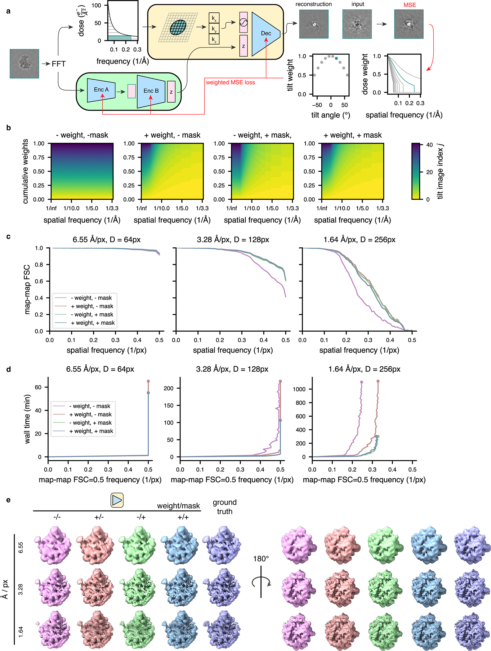
(a) Graphical overview of the dose filtering scheme (applied upstream of the decoder) and dose and tilt weighting scheme (applied during reconstruction error calculation) for a single representative tilt image. Filtering: the fixed optimal exposure curve is used to determine which spatial frequencies will be considered as a function of dose; the decoder processes only Fourier lattice coordinates within this mask (green lattice circle). Weighting: the squared error of the reconstructed Fourier slice is weighted per-frequency by the exposure-dependent amplitude attenuation curve and per-slice by the cosine of the corresponding stage tilt angle, before backpropagation of the mean squared error (red arrows).

(b) Relative weight of each tilt image assigned to a particle’s reconstruction error during model training as a function of spatial frequencies (x-axis), and tilt and dose, which are colored yellow to blue from low-to-high dose and tilt angle, assuming a dose symmetric tilt scheme (Hagen, Wan et al. 2017). Note that dose-filtering is applied upstream of the illustrated reconstruction weights.

(c) Map-map FSC of simulated class E large ribosomal subunit volumes (Davis, Tan et al. 2016) compared to tomoDRGN homogeneous network reconstructions in the presence or absence of the weighting or masking schemes at varying box and pixel sizes.

(d) Spatial frequencies corresponding to FSC=0.5 map-map correlation with the ground truth volume plotted against wall time for model training.

(e) Final tomoDRGN reconstructed volumes (left and center) and ground truth volumes (right) in the presence or absence of the weighting or masking schemes at box and pixel sizes assessed in panels (c) and (d).

Extended Data Fig. 2. Random selection of tilts per epoch allows flexible and robust model training for datasets with non-uniform numbers of tilt-images per particle.

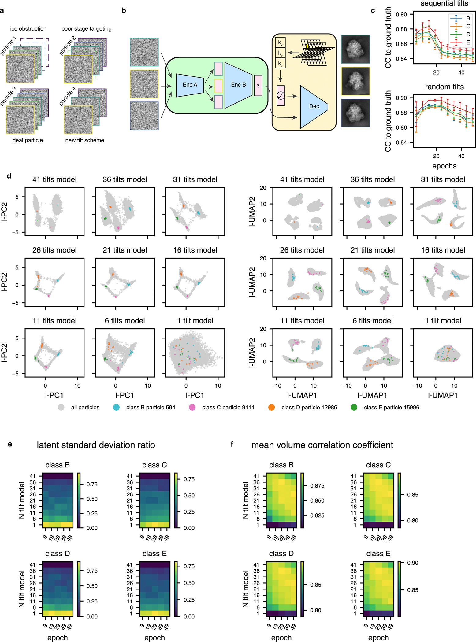
(a) Graphical summary of a dataset with non-uniform numbers of tilt images per particle. Here, the minimum number of tilt images for any particle is 3.

(b) Corresponding tomoDRGN network architecture for random sampling and ordering of 3 tilt images per particle.

(c) Mean per-class volumetric correlation coefficient for identical tomoDRGN models trained on 41 sequentially sampled tilts (top) or 41 randomly sampled tilts (bottom). At 5 epoch intervals, 25 random volumes were generated from each class for correlation coefficient calculation to ground truth ribosome assembly intermediate volumes (classes B-E). Error bars denote standard error of the mean CC.

(d) Nine tomoDRGN models with identical architectures were trained with the indicated number of tilts sampled per particle (total available tilts = 41). PCA (left) and UMAP (right) dimensionality reduction of each final epoch’s latent embeddings. Once trained, up to 10 randomly sampled and permuted tilt images for one representative particle from each volume class were embedded using the corresponding pretrained tomoDRGN model and are superimposed as colored points. Note increased dispersion of colored points as number of tilts sampled during training decreased.

(e) For each ribosomal large subunit class (B-E), 25 particles were randomly selected and up to 10 subsets of their tilt images were randomly sampled and permuted as in (d). In the heatmap, row indices refer to models trained in (d) using different numbers of sampled tilts (1–41), and columns denote epochs of training with that model. For each particle, each tilt subset was evaluated with the corresponding tomoDRGN model and the ratio of standard deviations of each particle’s 10 latent embeddings to all particles’ latent embeddings was calculated. The mean ratio across all particles, which measures the dispersion of encoder embeddings, is plotted per ribosomal LSU class. Here, lower dispersion indicates better performance.

(f) Particles and tilt subsets were selected as in (e). At each indicated epoch of training, the corresponding tomoDRGN model was used to generate volumes for each particle’s tilt subsets. For each such volume, the correlation coefficient was calculated between that volume and the corresponding ground truth volume. The mean across all particles at each epoch for each model is shown as a heatmap per ribosomal LSU class. Here, higher CC indicates improved performance.

Extended Data Fig. 3. TomoDRGN and MAVEn identify structural variations within HIV Gag lattice.

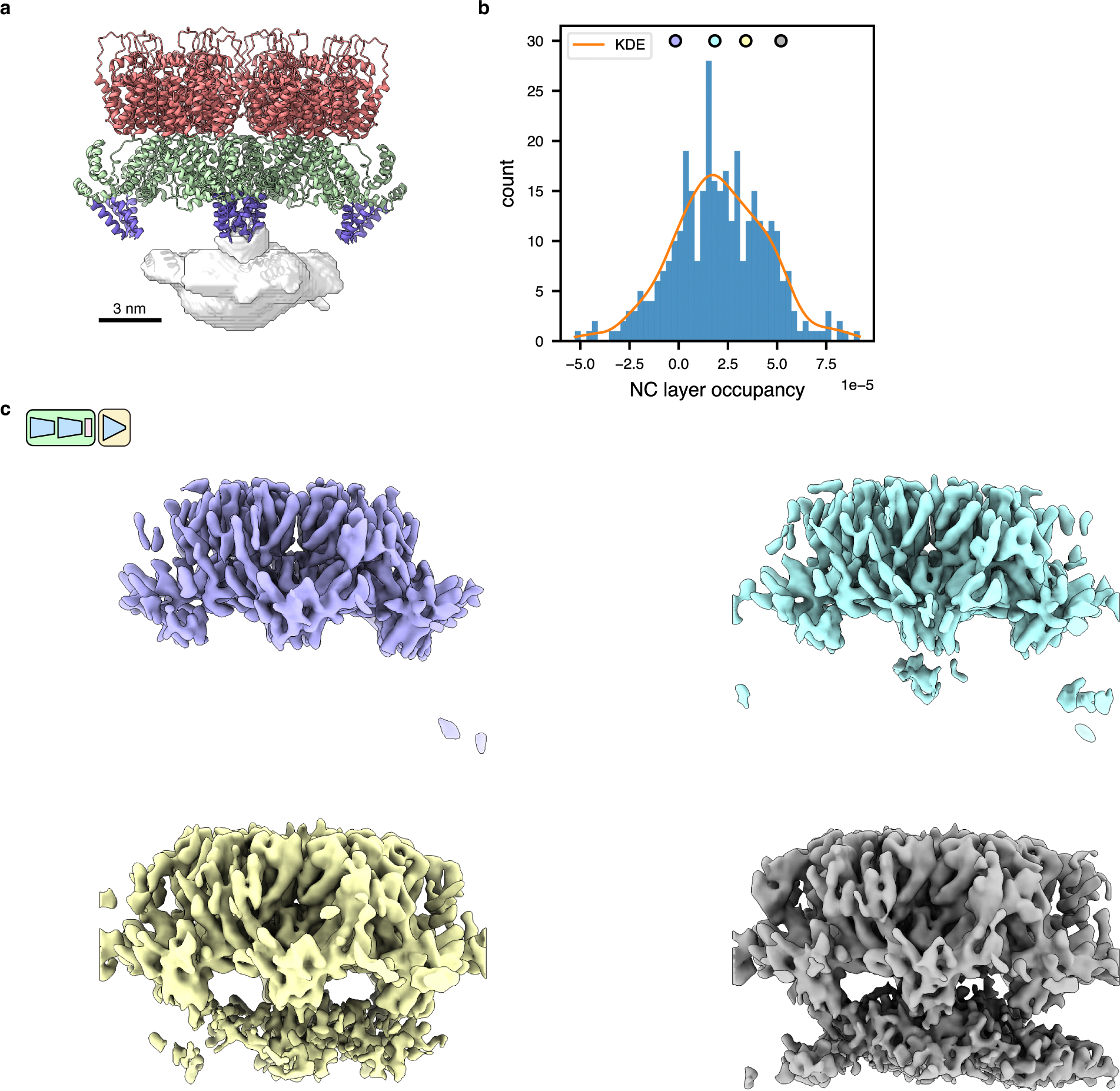
(a) Mask used for MAVEn-based occupancy analysis of NC layer density (gray, translucent). PDB: 5L93 is shown for reference, with CA-NTD colored salmon, CA-CTD colored green, and CA-SP1 helix colored purple.

(b) Histogram and kernel density estimate of NC layer occupancy across 500 volumes sampled from the trained tomoDRGN model, excluding junk particles (see Fig 3g).

(c) Representative volumes sampling along the NC occupancy histogram, colored as indicated in (b). Volumes are rendered at constant isosurface and same pose as in (a).

Extended Data Fig. 4. TomoDRGN identifies non-ribosomal particles picked from EMPIAR-10499 tomograms.

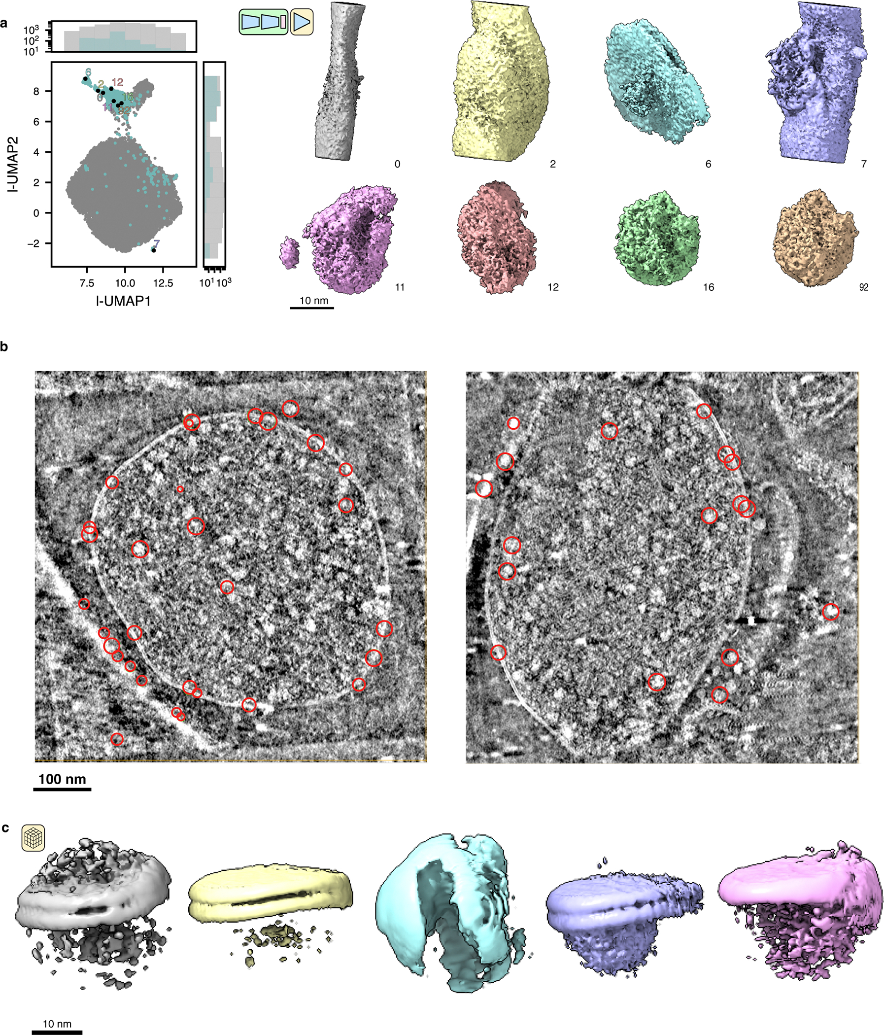
(a) Latent UMAP and corresponding sampled volumes from tomoDRGN heterogeneous network training from Fig. 5a. Eight representative non-ribosomal particles identified through manual inspection of k=100 k-means clustering of latent space are rendered at a constant isosurface and pose.

(b) Two tomograms are shown in slice view using Cube (https://github.com/dtegunov/cube) with locations of particles labeled as non-ribosomal annotated within each tomogram.

(c) RELION3-based multiclass (k=5) ab initio sub-tomogram volume generation using particles annotated as non-ribosomal via tomoDRGN (n=1,310).

Extended Data Fig. 5. TomoDRGN visualizes structurally heterogeneous disomes.

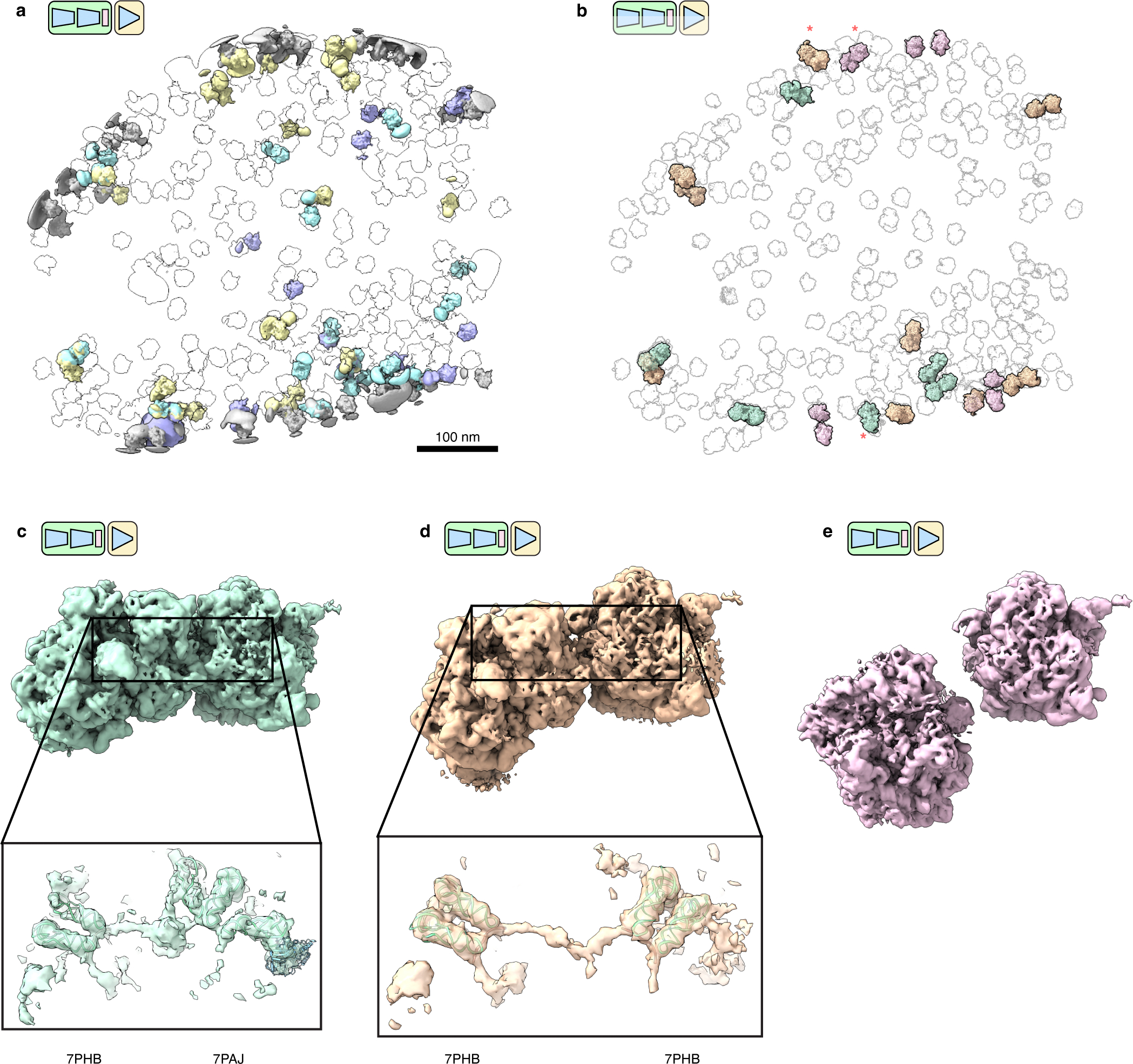
(a) An EMPIAR-10499 tomogram reconstructed with tomoDRGN intermolecular volumes. Volumes were generated for each ribosome using the trained intermolecular tomoDRGN model, colored as in Fig. 6a, and positioned correspondingly in the source tomogram. Transparent ribosomes correspond to free 50S and 70S ribosomes as annotated in Fig. 6a.

(b) The same tomogram as in panel (a) reconstructed with tomoDRGN intramolecular volumes. Volumes were generated for each ribosome using the trained intramolecular tomoDRGN model (Fig 5d). Pairs of volumes that were colored as disomes or trisomes and that exhibited mutually overlapping main and adjacent monosomes when mapped back to the tomogram in panel (a) were combined in ChimeraX (n=21 disomes). Disomes are colored by manual classification into three classes with representative volumes indicated with asterisks and shown in panels (c-e).

(c) A representative disome exhibiting continuous mRNA density between the two monosomes, including unattributed globular density along the mRNA (n=7 disomes). Density of each monosome fit by the indicated atomic model, excluding tRNA, mRNA, and elongation factors, has been removed using ChimeraX’s zone functionality (Inset).

(d) A representative disome exhibiting continuous mRNA density between the two monosomes (n=9 disomes). Inset as in panel (c).

(e) A representative ribosome pair with no apparent structural contact between the two monosomes (n=5 disomes). Inset as in panel (c).

Extended Data Fig. 6. Comparison of tomoDRGN-generated volumes to traditional sub-tomogram averaged volumes.

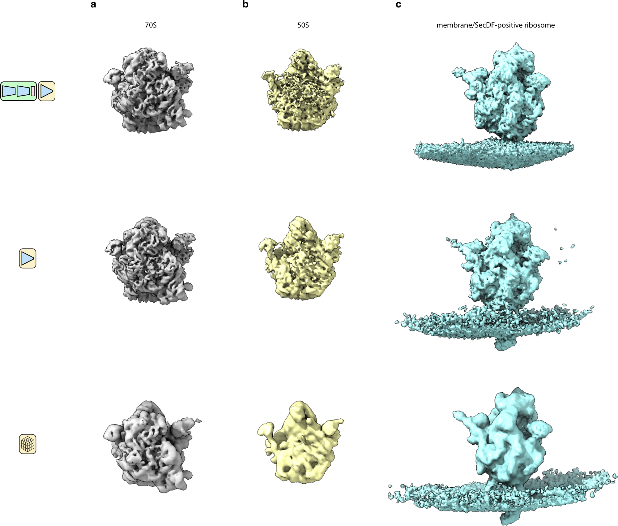
Comparison of volumes generated by a full tomoDRGN network (row 1), an isolated decoder neural network (row 2), or traditional sub-tomogram averaging (row 3). A full tomoDRGN network was trained on the heterogeneous ribosomal particle stack (row 1, n=20,981, see Figs. 5d and 6a) and representative volumes are depicted. Separate tomoDRGN homogeneous decoder networks were trained on one of three homogeneous substacks corresponding to (a) 70S particles (n=20,129); (b) 50S particles (n=852); or (c) SecDF-positive ribosomes (n=380). Traditional STA was also performed on each of these three particles stacks.

Extended Data Fig. 7. CryoDRGN fails to consistently encode structural heterogeneity using a simulated tilt series dataset.

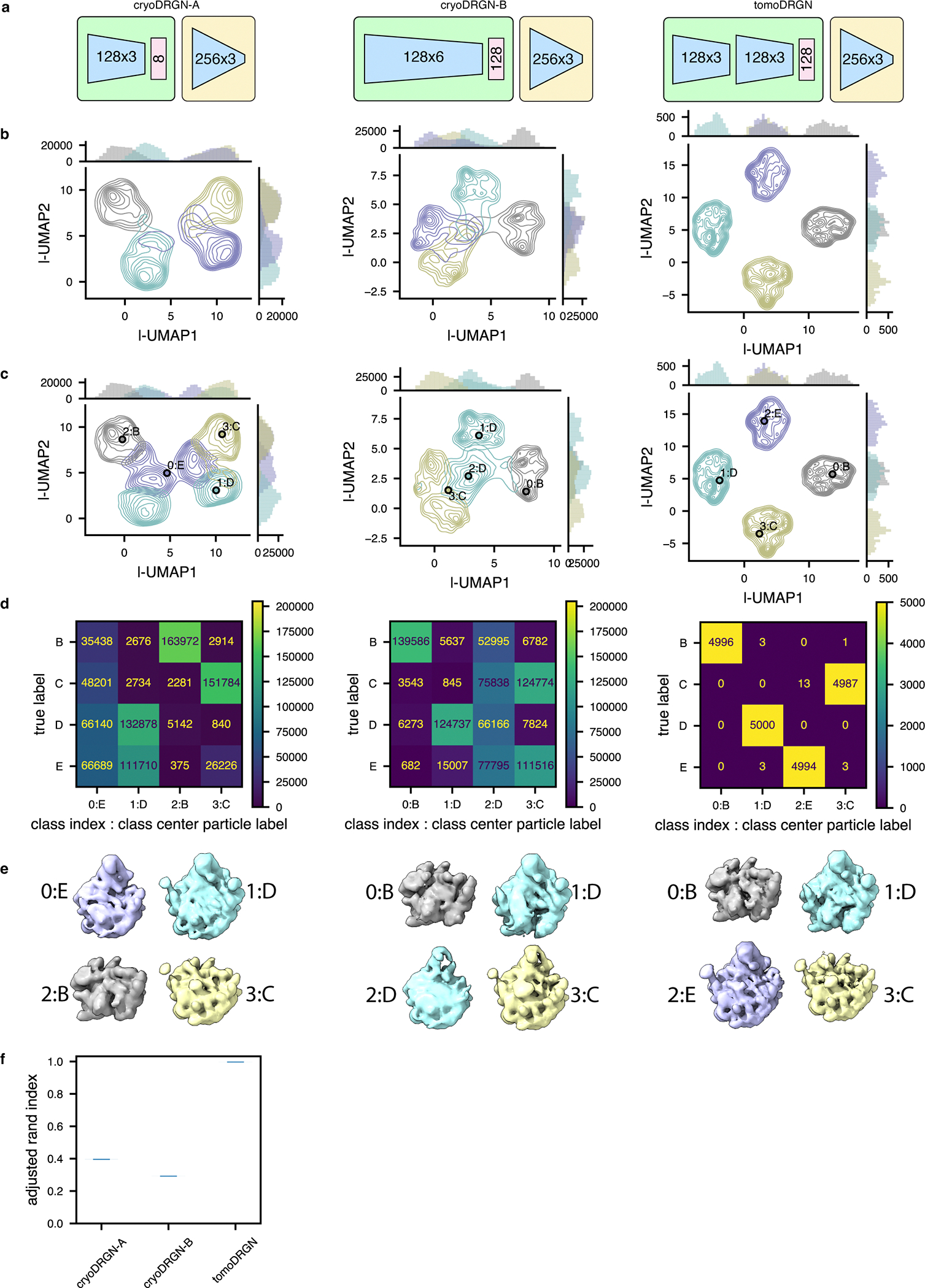
(a) Schematic of two cryoDRGN network architectures that were tested, and the tomoDRGN architecture used in Fig. 2c–e. Each model was trained using the same simulated dataset of ribosome large subunit assembly classes B-E (Davis, Tan et al. 2016) consisting of 41 tilt images for each of 5,000 particles for each of the four assembly states and thus the dataset was treated by cryoDRGN as n=820,000 images (see Methods).

(b) UMAP of final epoch latent embeddings of each particle image, with kernel density estimates independently estimated and plotted for each of the four ground truth assembly states.

(c) UMAP of final epoch latent embedding with k=4 k-means latent classification of the resulting latent space. KDEs were independently estimated and plotted for each of the four k-means classes. The predicted labels are annotated by both the k-means class index (0–3) and corresponding ground truth class label (B-E) of the central particle within each k-means class.

(d) Confusion matrix of ground truth class labels versus k=4 k-means latent classification.

(e) Volumes sampled at the k=4 k-means cluster centers illustrated in (c). Volumes are annotated by the k-means class index and ground truth class label and colored by the ground truth class label.

(f) Violin plot of consistency of k=4 k-means clustering of each model by Adjusted Rand Index (Hubert and Arabie 1985) (n = 100 randomly seeded initializations, higher values correspond to greater fidelity to ground truth classification).

Extended Data Fig. 8. CryoDRGN learns errant structural heterogeneity in an exemplar tomographic dataset.

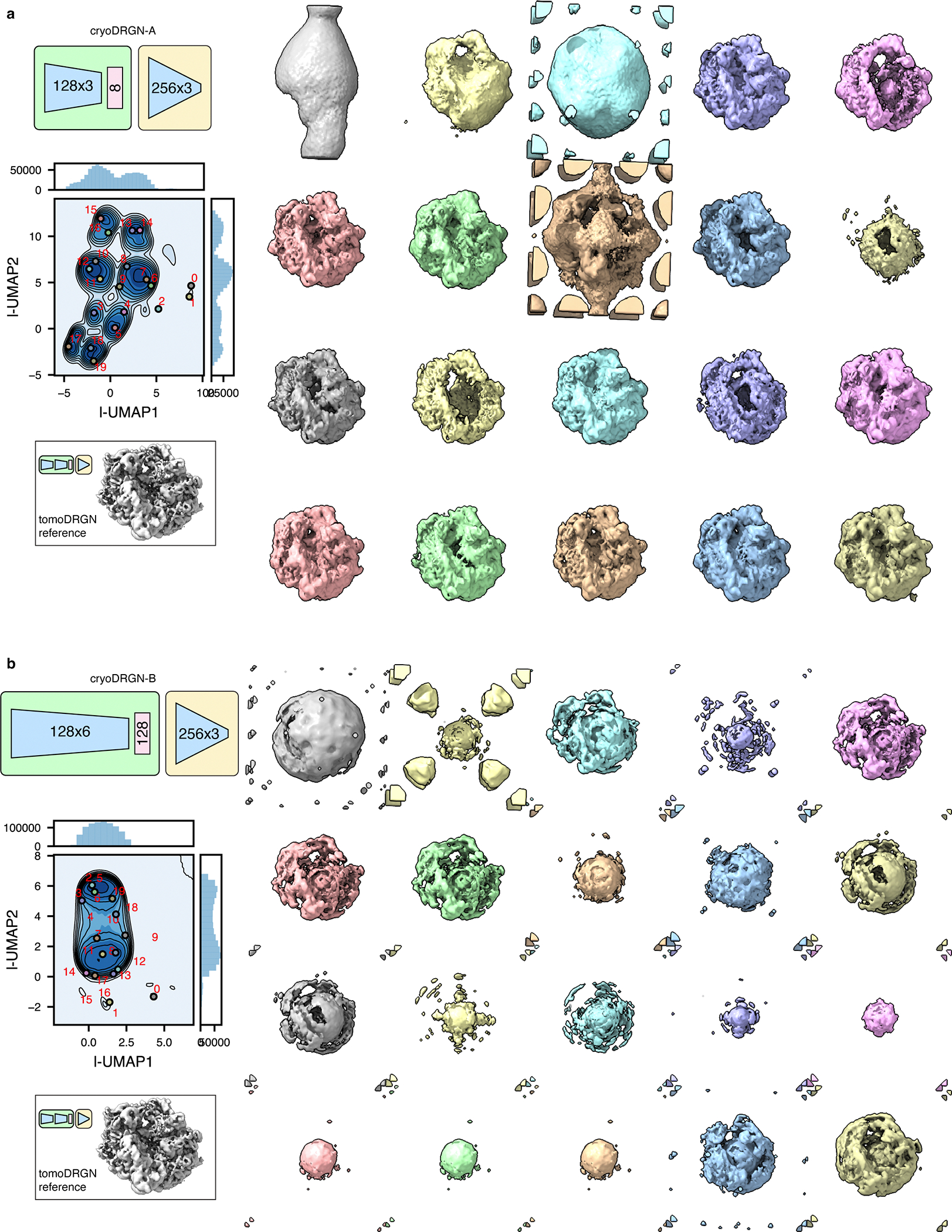
Two cryoDRGN models (a, b) were trained on the unfiltered particle stack of Mycoplasma pneumoniae ribosomes from Fig. 5a (n = 22,291 particles, treated as n = 913,931 images). The latent space is shown as a KDE plot following UMAP dimensionality reduction, with k=20 k-means class center particles annotated (left) and corresponding volumes visualized (right). Note that many putative 70S particles lack density in the particle core. A reference 70S volume sampled from tomoDRGN’s model in Fig. 5a is shown in the same pose for comparison.

Extended Data Fig. 9. CryoDRGN’s learned latent space embeddings exhibit undesirable correlations with tilt image index.

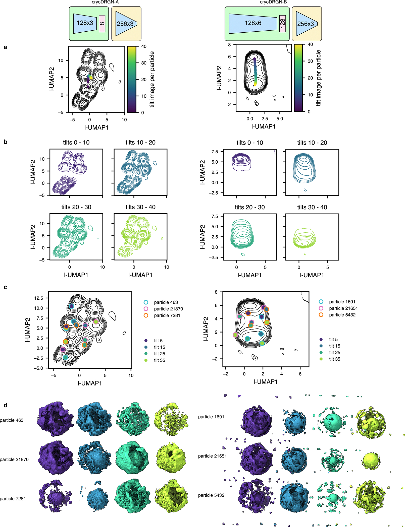
(a) Two cryoDRGN models were tested on the unfiltered particle stack of Mycoplasma pneumoniae ribosomes from Fig. 5a. The latent space is shown as a KDE plot following UMAP dimensionality reduction. The latent embeddings were binned by the tilt image index, and the median value across each bin is annotated.

(b) KDEs from panel A replotted after binning by tilt image index quartiles.

(c) KDEs from panel A with annotated positions corresponding to three representative particles evaluated using their 5^th, 15^th, 25^th, or 35^th tilt images.

(d) Volumes generated from cryoDRGN using the latent embeddings highlighted in panel C.

Extended Data Fig. 10. Assessment of tomoDRGN sensitivity to pose accuracy.

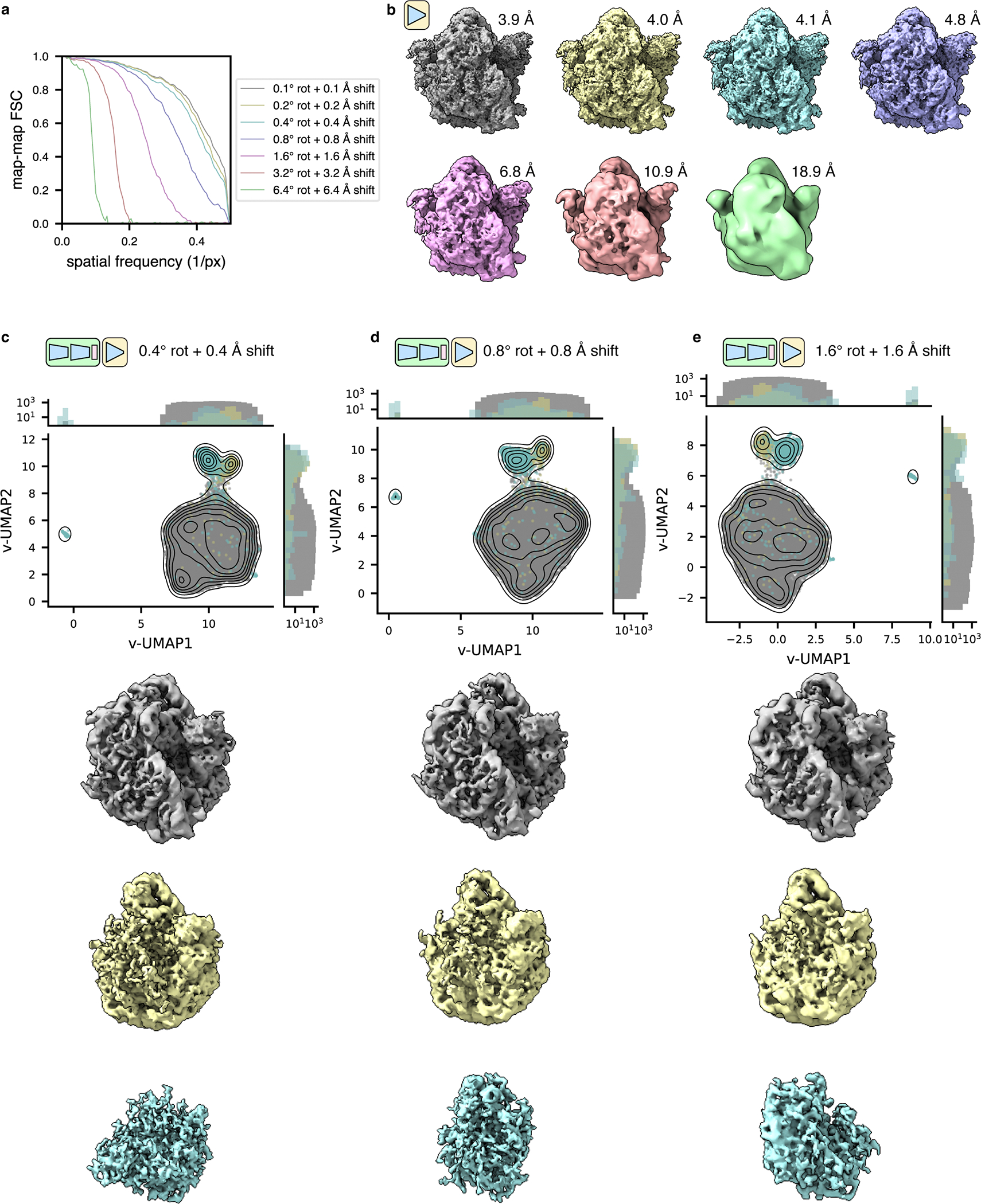
(a) The unfiltered stack of EMPIAR-10499 ribosomes in situ from Fig. 5a was used to train a series of tomoDRGN decoder-only models with increasing levels of random perturbations from STA-derived, “ground truth” rotation and translation poses (see Methods). The resulting map-map FSC curves against the STA ribosomal reconstruction are shown.

(b) Final tomoDRGN decoder-only reconstructed volumes corresponding to the FSC curves shown in (a). Volumes are lowpass filtered to the resolution where their map-map FSC to the STA ribosomal reconstruction crossed 0.5.

(c, d, e) UMAP of first 128 principal components of volume ensembles consisting of volumes generated for every particle, using tomoDRGN models trained on EMPIAR-10499 unfiltered ribosome stacks with indicated levels of pose perturbation. Particles annotated as 70S, 50S, and NR are colored as in Fig. 5c, with representative volumes of each class shown below. Note that NR particles are expected to be structurally diverse.

DATA AVAILABILITY

Extracted particle sub-tomograms from reprocessing of EMPIAR-10499 have been deposited as EMPIAR-11843. Requisite EMDB volumes and PDB models to generate synthetic data using cryoSRPNT as described in the methods are deposited at https://zenodo.org/doi/10.5281/zenodo.10076628. The trained models, latent embeddings, and particle classifications used to analyze all datasets presented have been deposited at https://zenodo.org/doi/10.5281/zenodo.10076628 for simulated datasets and https://zenodo.org/doi/10.5281/zenodo.10093310 for experimental datasets. Maps corresponding to C1 holoferritin and C1 apoferritin from EMPIAR-10491 generated in M have been deposited as EMD-43285 and EMD-43286. The map of secDF-associated 70S ribosome from EMPIAR-10499 generated in RELION has been deposited as EMD-43287.

REFERENCES

- 1.Bai XC, McMullan G & Scheres SH How cryo-EM is revolutionizing structural biology. Trends Biochem Sci 40, 49–57 (2015). [DOI] [PubMed] [Google Scholar]
- 2.Murata K & Wolf M Cryo-electron microscopy for structural analysis of dynamic biological macromolecules. Biochim Biophys Acta Gen Subj 1862, 324–334 (2018). [DOI] [PubMed] [Google Scholar]
- 3.Cheng Y, Grigorieff N, Penczek PA & Walz T A primer to single-particle cryo-electron microscopy. Cell 161, 438–449 (2015). [DOI] [PMC free article] [PubMed] [Google Scholar]
- 4.Zhong ED, Bepler T, Berger B & Davis JH CryoDRGN: reconstruction of heterogeneous cryo-EM structures using neural networks. Nat Methods 18, 176–185 (2021). [DOI] [PMC free article] [PubMed] [Google Scholar]
- 5.Punjani A & Fleet DJ 3D variability analysis: Resolving continuous flexibility and discrete heterogeneity from single particle cryo-EM. J Struct Biol 213, 107702 (2021). [DOI] [PubMed] [Google Scholar]
- 6.Chen M & Ludtke SJ Deep learning-based mixed-dimensional Gaussian mixture model for characterizing variability in cryo-EM. Nat Methods 18, 930–936 (2021). [DOI] [PMC free article] [PubMed] [Google Scholar]
- 7.Dashti A et al. Retrieving functional pathways of biomolecules from single-particle snapshots. Nat Commun 11, 4734 (2020). [DOI] [PMC free article] [PubMed] [Google Scholar]
- 8.Kinman LF, Powell BM, Zhong ED, Berger B & Davis JH Uncovering structural ensembles from single-particle cryo-EM data using cryoDRGN. Nat Protoc 18, 319–339 (2023). [DOI] [PMC free article] [PubMed] [Google Scholar]
- 9.Sun J, Kinman LF, Jahagirdar D, Ortega J & Davis JH KsgA facilitates ribosomal small subunit maturation by proofreading a key structural lesion. Nat Struct Mol Biol (2023). [DOI] [PMC free article] [PubMed] [Google Scholar]
- 10.Asano S, Engel BD & Baumeister W In Situ Cryo-Electron Tomography: A Post-Reductionist Approach to Structural Biology. J Mol Biol 428, 332–343 (2016). [DOI] [PubMed] [Google Scholar]
- 11.Lovatt M, Leistner C & Frank RAW Bridging length scales from molecules to the whole organism by cryoCLEM and cryoET. Faraday Discuss (2022). [DOI] [PMC free article] [PubMed] [Google Scholar]
- 12.Xue L et al. Visualizing translation dynamics at atomic detail inside a bacterial cell. Nature 610, 205–211 (2022). [DOI] [PMC free article] [PubMed] [Google Scholar]
- 13.Gemmer M et al. Visualization of translation and protein biogenesis at the ER membrane. Nature 614, 160–167 (2023). [DOI] [PMC free article] [PubMed] [Google Scholar]
- 14.Hoffmann PC et al. Structures of the eukaryotic ribosome and its translational states in situ. Nat Commun 13, 7435 (2022). [DOI] [PMC free article] [PubMed] [Google Scholar]
- 15.Zhang P Advances in cryo-electron tomography and subtomogram averaging and classification. Curr Opin Struct Biol 58, 249–258 (2019). [DOI] [PMC free article] [PubMed] [Google Scholar]
- 16.Castano-Diez D & Zanetti G In situ structure determination by subtomogram averaging. Curr Opin Struct Biol 58, 68–75 (2019). [DOI] [PMC free article] [PubMed] [Google Scholar]
- 17.Bharat TA & Scheres SH Resolving macromolecular structures from electron cryo-tomography data using subtomogram averaging in RELION. Nat Protoc 11, 2054–65 (2016). [DOI] [PMC free article] [PubMed] [Google Scholar]
- 18.Pyle E & Zanetti G Current data processing strategies for cryo-electron tomography and subtomogram averaging. Biochem J 478, 1827–1845 (2021). [DOI] [PMC free article] [PubMed] [Google Scholar]
- 19.Castano-Diez D, Kudryashev M, Arheit M & Stahlberg H Dynamo: a flexible, user-friendly development tool for subtomogram averaging of cryo-EM data in high-performance computing environments. J Struct Biol 178, 139–51 (2012). [DOI] [PubMed] [Google Scholar]
- 20.Hrabe T et al. PyTom: a python-based toolbox for localization of macromolecules in cryo-electron tomograms and subtomogram analysis. J Struct Biol 178, 177–88 (2012). [DOI] [PubMed] [Google Scholar]
- 21.Nickell S et al. TOM software toolbox: acquisition and analysis for electron tomography. J Struct Biol 149, 227–34 (2005). [DOI] [PubMed] [Google Scholar]
- 22.Scheres SHW, Melero R, Valle M & Carazo JM Averaging of electron subtomograms and random conical tilt reconstructions through likelihood optimization. Structure 17, 1563–1572 (2009). [DOI] [PMC free article] [PubMed] [Google Scholar]
- 23.Winkler H et al. Tomographic subvolume alignment and subvolume classification applied to myosin V and SIV envelope spikes. J Struct Biol 165, 64–77 (2009). [DOI] [PMC free article] [PubMed] [Google Scholar]
- 24.Bartesaghi A et al. Classification and 3D averaging with missing wedge correction in biological electron tomography. J Struct Biol 162, 436–50 (2008). [DOI] [PMC free article] [PubMed] [Google Scholar]
- 25.Walz J et al. Electron Tomography of Single Ice-Embedded Macromolecules: Three-Dimensional Alignment and Classification. J Struct Biol 120, 387–95 (1997). [DOI] [PubMed] [Google Scholar]
- 26.Zivanov J et al. A Bayesian approach to single-particle electron cryo-tomography in RELION-4.0. Elife 11(2022). [DOI] [PMC free article] [PubMed] [Google Scholar]
- 27.Tegunov D, Xue L, Dienemann C, Cramer P & Mahamid J Multi-particle cryo-EM refinement with M visualizes ribosome-antibiotic complex at 3.5 A in cells. Nat Methods 18, 186–193 (2021). [DOI] [PMC free article] [PubMed] [Google Scholar]
- 28.Chen M et al. A complete data processing workflow for cryo-ET and subtomogram averaging. Nat Methods 16, 1161–1168 (2019). [DOI] [PMC free article] [PubMed] [Google Scholar]
- 29.Himes BA & Zhang P emClarity: software for high-resolution cryo-electron tomography and subtomogram averaging. Nat Methods 15, 955–961 (2018). [DOI] [PMC free article] [PubMed] [Google Scholar]
- 30.Jiang W et al. A transformation clustering algorithm and its application in polyribosomes structural profiling. Nucleic Acids Res 50, 9001–9011 (2022). [DOI] [PMC free article] [PubMed] [Google Scholar]
- 31.Cheng J, Wu C, Li J, Yang Q & Zhang X Visualizing translating dynamics in situ at high spatial and temporal resolution in eukaryotic cells. bioRxiv, 2023.07.12.548775 (2023). [Google Scholar]
- 32.Fedry J et al. Visualization of translation reorganization upon persistent collision stress in mammalian cells. bioRxiv, 2023.03.23.533914 (2023). [DOI] [PMC free article] [PubMed] [Google Scholar]
- 33.Harastani M, Eltsov M, Leforestier A & Jonic S TomoFlow: Analysis of Continuous Conformational Variability of Macromolecules in Cryogenic Subtomograms based on 3D Dense Optical Flow. J Mol Biol 434, 167381 (2022). [DOI] [PubMed] [Google Scholar]
- 34.Harastani M, Eltsov M, Leforestier A & Jonic S HEMNMA-3D: Cryo Electron Tomography Method Based on Normal Mode Analysis to Study Continuous Conformational Variability of Macromolecular Complexes. Front Mol Biosci 8, 663121 (2021). [DOI] [PMC free article] [PubMed] [Google Scholar]
- 35.Stolken M et al. Maximum likelihood based classification of electron tomographic data. J Struct Biol 173, 77–85 (2011). [DOI] [PubMed] [Google Scholar]
- 36.Bartesaghi A, Lecumberry F, Sapiro G & Subramaniam S Protein secondary structure determination by constrained single-particle cryo-electron tomography. Structure 20, 2003–13 (2012). [DOI] [PMC free article] [PubMed] [Google Scholar]
- 37.Balyschew N et al. Streamlined Structure Determination by Cryo-Electron Tomography and Subtomogram Averaging using TomoBEAR. bioRxiv, 2023.01.10.523437 (2023). [DOI] [PMC free article] [PubMed] [Google Scholar]
- 38.Kingma DP & Welling M Auto-encoding variational bayes. arXiv preprint arXiv:1312.6114 (2013). [Google Scholar]
- 39.Zhong ED, Bepler T, Davis JH & Berger B Reconstructing continuous distributions of 3D protein structure from cryo-EM images. arXiv preprint arXiv:1909.05215 (2019). [Google Scholar]
- 40.Bepler T, Zhong E, Kelley K, Brignole E & Berger B Explicitly disentangling image content from translation and rotation with spatial-VAE. Advances in Neural Information Processing Systems 32(2019). [Google Scholar]
- 41.Higgins I et al. beta-vae: Learning basic visual concepts with a constrained variational framework. in International conference on learning representations (2016). [Google Scholar]
- 42.Becht E et al. Dimensionality reduction for visualizing single-cell data using UMAP. Nat Biotechnol (2018). [DOI] [PubMed] [Google Scholar]
- 43.Grant T & Grigorieff N Measuring the optimal exposure for single particle cryo-EM using a 2.6 A reconstruction of rotavirus VP6. Elife 4, e06980 (2015). [DOI] [PMC free article] [PubMed] [Google Scholar]
- 44.Bharat TAM, Russo CJ, Lowe J, Passmore LA & Scheres SHW Advances in Single-Particle Electron Cryomicroscopy Structure Determination applied to Sub-tomogram Averaging. Structure 23, 1743–1753 (2015). [DOI] [PMC free article] [PubMed] [Google Scholar]
- 45.Hayward SB & Glaeser RM Radiation damage of purple membrane at low temperature. Ultramicroscopy 04, 201–10 (1979). [DOI] [PubMed] [Google Scholar]
- 46.Glaeser RM Prospects for extending the resolution limit of the electron microscope. J Microsc 117, 77–91 (1979). [DOI] [PubMed] [Google Scholar]
- 47.Baxter WT, Grassucci RA, Gao H & Frank J Determination of signal-to-noise ratios and spectral SNRs in cryo-EM low-dose imaging of molecules. J Struct Biol 166, 126–32 (2009). [DOI] [PMC free article] [PubMed] [Google Scholar]
- 48.Davis JH et al. Modular Assembly of the Bacterial Large Ribosomal Subunit. Cell 167, 1610–1622 e15 (2016). [DOI] [PMC free article] [PubMed] [Google Scholar]
- 49.Davis JH & Williamson JR Structure and dynamics of bacterial ribosome biogenesis. Philos Trans R Soc Lond B Biol Sci 372(2017). [DOI] [PMC free article] [PubMed] [Google Scholar]
- 50.Guo H & Rubinstein JL Structure of ATP synthase under strain during catalysis. Nat Commun 13, 2232 (2022). [DOI] [PMC free article] [PubMed] [Google Scholar]
- 51.Schur FK et al. An atomic model of HIV-1 capsid-SP1 reveals structures regulating assembly and maturation. Science 353, 506–8 (2016). [DOI] [PubMed] [Google Scholar]
- 52.Mendonca L et al. CryoET structures of immature HIV Gag reveal six-helix bundle. Commun Biol 4, 481 (2021). [DOI] [PMC free article] [PubMed] [Google Scholar]
- 53.Stojkovic V et al. Assessment of the nucleotide modifications in the high-resolution cryo-electron microscopy structure of the Escherichia coli 50S subunit. Nucleic Acids Res 48, 2723–2732 (2020). [DOI] [PMC free article] [PubMed] [Google Scholar]
- 54.Fromm SA et al. The translating bacterial ribosome at 1.55 A resolution generated by cryo-EM imaging services. Nat Commun 14, 1095 (2023). [DOI] [PMC free article] [PubMed] [Google Scholar]
- 55.Chen SS, Sperling E, Silverman JM, Davis JH & Williamson JR Measuring the dynamics of E. coli ribosome biogenesis using pulse-labeling and quantitative mass spectrometry. Mol Biosyst 8, 3325–34 (2012). [DOI] [PMC free article] [PubMed] [Google Scholar]
- 56.Turk M & Baumeister W The promise and the challenges of cryo-electron tomography. FEBS Lett 594, 3243–3261 (2020). [DOI] [PubMed] [Google Scholar]
- 57.Saito K et al. Ribosome collisions induce mRNA cleavage and ribosome rescue in bacteria. Nature 603, 503–508 (2022). [DOI] [PMC free article] [PubMed] [Google Scholar]
- 58.Rangan R et al. Deep reconstructing generative networks for visualizing dynamic biomolecules inside cells. bioRxiv, 2023.08.18.553799 (2023). [DOI] [PubMed] [Google Scholar]
- 59.Vasyliuk D et al. Conformational landscape of the yeast SAGA complex as revealed by cryo-EM. Sci Rep 12, 12306 (2022). [DOI] [PMC free article] [PubMed] [Google Scholar]
- 60.Sekne Z, Ghanim GE, van Roon AM & Nguyen THD Structural basis of human telomerase recruitment by TPP1-POT1. Science 375, 1173–1176 (2022). [DOI] [PMC free article] [PubMed] [Google Scholar]
- 61.Rice G, Wagner T, Stabrin M & Raunser S TomoTwin: Generalized 3D Localization of Macromolecules in Cryo-electron Tomograms with Structural Data Mining. bioRxiv, 2022.06.24.497279 (2022). [DOI] [PMC free article] [PubMed] [Google Scholar]
- 62.Tancik M et al. Fourier features let networks learn high frequency functions in low dimensional domains. Advances in Neural Information Processing Systems 33, 7537–7547 (2020). [Google Scholar]
- 63.Bracewell RN Strip integration in radio astronomy. Australian Journal of Physics 9, 198–217 (1956). [Google Scholar]
- 64.Moebel E et al. Deep learning improves macromolecule identification in 3D cellular cryo-electron tomograms. Nat Methods 18, 1386–1394 (2021). [DOI] [PubMed] [Google Scholar]
- 65.Luo Z, Ni F, Wang Q & Ma J OPUS-DSD: deep structural disentanglement for cryo-EM single-particle analysis. Nat Methods (2023). [DOI] [PMC free article] [PubMed] [Google Scholar]
- 66.Tegunov D & Cramer P Real-time cryo-electron microscopy data preprocessing with Warp. Nat Methods 16, 1146–1152 (2019). [DOI] [PMC free article] [PubMed] [Google Scholar]
- 67.Zheng S et al. AreTomo: An integrated software package for automated marker-free, motion-corrected cryo-electron tomographic alignment and reconstruction. J Struct Biol X 6, 100068 (2022). [DOI] [PMC free article] [PubMed] [Google Scholar]
- 68.Burt A, Gaifas L, Dendooven T & Gutsche I A flexible framework for multi-particle refinement in cryo-electron tomography. PLoS Biol 19, e3001319 (2021). [DOI] [PMC free article] [PubMed] [Google Scholar]
- 69.Hubert L & Arabie P Comparing partitions. Journal of Classification 2, 193–218 (1985). [Google Scholar]
- 70.Afonine PV et al. New tools for the analysis and validation of cryo-EM maps and atomic models. Acta Crystallogr D Struct Biol 74, 814–840 (2018). [DOI] [PMC free article] [PubMed] [Google Scholar]
- 71.Pettersen EF et al. UCSF ChimeraX: Structure visualization for researchers, educators, and developers. Protein Sci 30, 70–82 (2021). [DOI] [PMC free article] [PubMed] [Google Scholar]
- 72.Goddard TD et al. UCSF ChimeraX: Meeting modern challenges in visualization and analysis. Protein Sci 27, 14–25 (2018). [DOI] [PMC free article] [PubMed] [Google Scholar]
- 73.Petrov AS et al. Secondary structures of rRNAs from all three domains of life. PLoS One 9, e88222 (2014). [DOI] [PMC free article] [PubMed] [Google Scholar]
Associated Data
This section collects any data citations, data availability statements, or supplementary materials included in this article.
Supplementary Materials
Data Availability Statement